A primer on network meta-analysis with emphasis on mental health

Abstract

Objective

A quantitative synthesis of evidence via standard pair-wise meta-analysis lies on the top of the hierarchy for evaluating the relative effectiveness or safety between two interventions. In most healthcare problems, however, there is a plethora of competing interventions. Network meta-analysis allows to rank competing interventions and evaluate their relative effectiveness even if they have not been compared in an individual trial. The aim of this paper is to explain and discuss the main features of this statistical technique.

Methods

We present the key assumptions underlying network meta-analysis and the graphical methods to visualise results and information in the network. We used one illustrative example that compared the relative effectiveness of 15 antimanic drugs and placebo in acute mania.

Results

A network plot allows to visualise how information flows in the network and reveals important information about network geometry. Discrepancies between direct and indirect evidence can be detected using inconsistency plots. Relative effectiveness or safety of competing interventions can be presented in a league table. A contribution plot reveals the contribution of each direct comparison to each network estimate. A comparison-adjusted funnel plot is an extension of simple funnel plot to network meta-analysis. A rank probability matrix can be estimated to present the probabilities of all interventions assuming each rank and can be represented using rankograms and cumulative probability plots.

Conclusions

Network meta-analysis is very helpful in comparing the relative effectiveness and acceptability of competing treatments. Several issues, however, still need to be addressed when conducting a network meta-analysis for the results to be valid and correctly interpreted.

Introduction

Evidence-based practices are crucial in informing healthcare decisions as they provide evidence on the effectiveness and adverse effects of the available treatment options. A quantitative synthesis of research findings from randomised controlled trials (RCTs) via meta-analysis lies at the top of evidence based methods.¹ The benefits from meta-analysis are well established and include increased power, more precise effect estimates, and ability to generalise research findings and identify factors that modify the effect of an intervention (effect modifiers). In mental health, several meta-analyses have identified interventions that help people with mental disorders to attain better outcomes in terms of symptoms, functional status and quality of life. Examples of such interventions include psychosocial, psychological and pharmacological interventions.

Even within a class of interventions, there is a plethora of available options and they are not necessarily all equal. For example, Leucht et al² found that second generation antipsychotics differ in many ways and should not be treated as a homogeneous class of drugs. It is expected that in most mental disorders a systematic review would find many trials comparing different interventions and the clinical interest would not lie only in comparing a pair of them (eg, via traditional meta-analysis) or grouping them in large classes (eg, active interventions vs placebo, psychosocial vs pharmacological interventions) of possibly heterogeneous interventions. The main question is which intervention is the best or the worst (eg, in terms of efficacy) and under what circumstances (eg, for whom). A relatively new statistical technique, called network meta-analysis (NMA), can be employed to address these issues.^3–5 It is an extension of traditional pair-wise meta-analysis that allows synthesising studies that compare different interventions as long as these interventions form a connected network of evidence in which information flows not only directly but also indirectly. NMA yields summary estimates for the relative effectiveness between any pair of interventions by synthesising both direct and indirect evidence, and ranks them according to the outcome measured (eg, efficacy or safety). Systematic reviews that employ NMA are becoming more popular as initial doubt about the method fades away and user-friendly software becomes available.⁶ Statistical methodology is evolving and there are many review papers that provide guidelines on how to apply NMA, and how to present and interpret results.^7–10 There are an increasing number of NMAs conducted in mental health that assess the comparative efficacy and tolerability of competing treatments for various disorders.^11–14

Basic concepts and assumptions in NMA

A fundamental concept in NMA is that of an indirect comparison. If two treatments, A and B, have both been compared with a common treatment, say C, in two different sets of trials (A vs C and B vs C), then the relative effectiveness between A and B can be estimated indirectly via the common comparator C.¹⁵ For illustrative purposes, we will consider three active antipsychotics, namely haloperidol (H), olanzapine (O) and risperidone (R). If there are only studies comparing risperidone or olanzapine with haloperidol, the summary estimates are as follows:  and , where upper index refers to the source of evidence (direct in this case, but in theory it could be direct or indirect) and lower index refers to the treatment comparison; then, it is possible to yield the indirect evidence for the relative effectiveness between olanzapine and risperidone by subtracting the two summary estimates as follows: . Hence, even if there are no studies directly comparing olanzapine and risperidone (that means we cannot estimate ) we can still get an indirect estimate of the relative effectiveness between them. Bucher et al¹⁵ developed the idea of an indirect estimate and gave details on how to quantify their uncertainty and compute CIs. In a larger network of treatments, there is not necessarily only one indirect path from one intervention to another, as in the example we showed. If we had four antipsychotics, for example, adding paliperidone (P), we could get an indirect estimate for olanzapine versus risperidone through paliperidone, for example, O-P-R or through both haloperidol and paliperidone O-H-P-R. Another advantage of NMA is that it is possible to synthesise both indirect evidence and direct evidence into one pooled estimate, which is called mixed estimate. In a hypothetical network of studies directly comparing olanzapine with risperidone (), this estimate will be used along with the indirect estimate  to get a NMA estimate for the relative effectiveness between the two antipsychotics.

Indirect evidence is plausibly valid and accurate if the unit of analysis is measured without uncertainty (or with uncertainty caused only by random variation). If we have three people, A, B and C, and we know that B is 5 cm taller than A and C is 8 cm taller than A, we immediately know that C is 3 cm taller than B. In practice, trials usually report relative differences that are subject not only to random variation but also to variation due to clinical and methodological aspects of the trials. For example, it has been shown that antidepressants are more effective in severely depressed people.¹⁶ If two active antidepressants, A and B, are compared with placebo, but A is tested only in trials with more severely depressed patients and B is tested in trials with patients suffering from mild depression, the indirect estimate for A versus B will give biased results and would probably show a spurious advantage of A over B (see below for more explanations about this).

Even if participants are randomised within a RCT to receive one of the available treatments, NMA is by nature an observational process because treatment comparisons are not randomised across trials. We do not necessarily have the same distribution of trial characteristics across treatment comparisons. A key assumption in NMA is transitivity, which implies that the distribution of the effect modifiers is the same across treatment comparisons. Transitivity is not violated if the trial characteristic does not modify the effect of the interventions. If A versus B studies involve younger participants than A versus C studies, we can still get a valid indirect estimate for B versus C if age is not an effect modifier. By contrast, if effectiveness of interventions changes with age, an indirect estimate is invalid and results from NMA are misleading. The transitivity assumption may be challenged when we have interventions included in trials conducted in different time periods, for example, old and new interventions. There is ample evidence that older trials involve smaller sample sizes, are of worse quality and show exaggerated effects.^{17 18} Publication bias is also more evident in older interventions. The transitivity assumption has a statistical manifestation known as the consistency assumption. This assumption implies that direct and indirect evidence is in agreement. In practice, if three treatments, A, B and C, form a closed loop of evidence (any subset of interventions where each of that have been directly compared with one another), the consistency equation requires that  or that the direct estimate (left-hand side of the equation) equals the indirect estimate (right-hand side). The difference between direct and indirect evidence in a loop is called the inconsistency factor of the loop.

A working example

There are many aspects in a NMA that need to be addressed in a thorough analysis. Are the underlying assumptions valid? How to proceed if not? How to present and interpret results? To illustrate how to conduct a NMA, we will use a published NMA that includes 67 RCTs (16 073 patients) and compares 15 antimanic drugs and placebo in acute mania. There were two primary outcomes: the mean change on mania rating scales (efficacy) and the number of patients who dropped out (acceptability), both at 3 weeks. The former was measured on a continuous scale and standardised mean differences were synthesised, whereas the latter was dichotomous and ORs were synthesised. All analyses were performed in Stata¹⁹ using the mvmeta command²⁰ and a suite of commands for presenting and interpreting results from a NMA.²¹

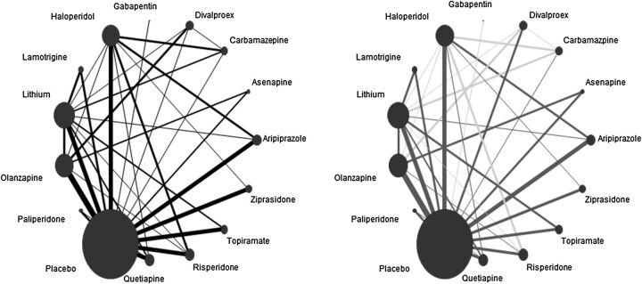
Network plot

The first step in a NMA is to understand the geometry of the network; that is, to understand which treatments have been compared directly in the included RCTs, how information flows indirectly and the contribution of certain interventions or treatment comparisons in the network. A standard tool to achieve these goals is a network plot that depicts the competing interventions by nodes and uses lines to connect those interventions that have been compared directly in a RCT. The size of the node can be used to represent extra information such as the number of studies involving this intervention or the number of participants who have been randomised to this intervention. The width of the lines can also be used to denote the number of studies for each comparisons or the number of participants observed in each comparison.

We can use the network plot to reveal information about characteristics that pertain to treatment comparisons. We may use different colours to represent trial characteristics that vary across treatment comparisons. Figure 1 shows two versions of the network plot. It is clear that most trials are placebo-controlled. From the active antimanics, haloperidol, lithium and olanzapine contribute significantly in the network. There are methods, not explored here, to determine exactly the contribution of each intervention or comparison in the network.^{21 22} The right-hand side plot of figure 1 conveys the same information but lines have been coloured according to publication date. A light grey colour for a treatment comparison refers to the fact that most studies for that comparison were published before 2003, whereas a dark grey colour means that the majority of studies were published from 2003 onwards. We observe that most studies comparing carbamazepine, divalproex, haloperidol and lithium to other drugs are compared in older studies.

Figure 1.

Network plot for efficacy. Size of nodes is proportional to the number of patients randomised to interventions. Thickness of lines is proportional to the number of studies contributing to the direct comparison. In the right-hand side plot, light grey lines denote that the majority of studies for that comparison were conducted before 2003, whereas dark grey lines denote that the majority of studies were conducted after 2003.

The risk of bias in studies included in a treatment comparison should affect the confidence we place on the direct estimate. Salanti et al²³ and Puhan et al²⁴ extended the methodology developed by the Grading of Recommendations, Assessment, Development and Evaluation (GRADE) working group for placing confidence in the treatment effect estimates from a NMA. In a network plot, we can use different colours in the lines to represent the level of confidence we place in a treatment comparison or in a specific item of the risk of bias tool.²¹

Network estimates

NMA allows estimating the relative effectiveness between any pair of interventions. In our example of 15 antimanic drugs, there are 105 relative effect estimates for each of the two outcomes (210 in total). One way to present results from a NMA is by drawing a square matrix, known as a league table, which contains all information about relative effectiveness and their uncertainty for all pairs of interventions (table 1). It is difficult to comprehend all the information from the league table but a closer look reveals that risperidone and haloperidol are more effective than most of the drugs and almost all drugs are more effective than lamotrigine, placebo, topiramate and gabapentin. Topiramate also ranks very low in terms of acceptability, and there is a significant difference between olanzapine and haloperidol in favour of olanzapine. From a clinical point of view, this is very important, because these two drugs are among the most effective ones.

Table 1.

Relative effect estimates for each pair of antimanic drugs accompanied by 95% CIs according to efficacy (lower diagonal) and acceptability (upper diagonal)

Risperidone

0.69 (0.45 to 1.07)

1.03 (0.68 to 1.56)

0.90 (0.46 to 1.76)

0.76 (0.37 to 1.43)

0.77 (0.48 to 1.25)

0.57 (0.36 to 0.91)

0.90 (0.55 to 1.48)

0.60 (0.32 to 1.13)

0.80 (0.49 to 1.33)

0.64 (0.38 to 1.08)

0.49 (0.24 to 0.97)

0.59 (0.41 to 0.85)

0.39 (0.23 to 0.67)

0.34 (0.11 to 0.99)

−0.01 (−0.17 to 0.16)

Haloperidol

1.49 (1.04 to 2.13)

1.30 (0.69 to 2.44)

1.04 (0.56 to 1.96)

1.12 (0.76 to 1.64)

0.82 (0.55 to 1.24)

1.30 (0.84 to 2.01)

0.87 (0.48 to 1.58)

1.16 (0.73 to 1.82)

0.92 (0.59 to 1.45)

0.70 (0.36 to 1.35)

0.85 (0.62 to 1.15)

0.57 (0.35 to 0.93)

0.48 (0.17 to 1.40)

−0.12 (−0.28 to 0.04)

−0.12 (−0.26 to 0.03)

Olanzapine

0.87 (0.47 to 1.61)

0.70 (0.38 to 1.31)

0.75 (0.50 to 1.12)

0.55 (0.38 to 0.81)

0.87 (0.57 to 1.33)

0.58 (0.34 to 0.99)

0.78 (0.53 to 1.15)

0.62 (0.40 to 0.97)

0.47 (0.25 to 0.89)

0.57 (0.44 to 0.74)

0.38 (0.24 to 0.61)

0.33 (0.11 to 0.93)

−0.19 (−0.42 to 0.04)

−0.18 (−0.40 to 0.03)

−0.07 (−0.28 to 0.14)

Paliperidone

0.80 (0.36 to 1.80)

0.86 (0.45 to 1.63)

0.63 (0.34 to 1.19)

1.00 (0.55 to 1.83)

0.67 (0.31 to 1.44)

0.89 (0.46 to 1.73)

0.71 (0.36 to 1.39)

0.54 (0.24 to 1.21)

0.65 (0.37 to 1.14)

0.44 (0.22 to 0.87)

0.37 (0.12 to 1.19)

−0.19 (−0.46 to 0.08)

−0.19 (−0.44 to 0.06)

−0.07 (−0.32 to 0.18)

−0.00 (−0.30 to 0.30)

Carbamazepine

1.07 (0.56 to 2.05)

0.79 (0.43 to 1.46)

1.24 (0.64 to 2.42)

0.83 (0.38 to 1.81)

1.11 (0.57 to 2.14)

0.88 (0.44 to 1.76)

0.67 (0.30 to 1.51)

0.81 (0.45 to 1.45)

0.54 (0.27 to 1.08)

0.46 (0.14 to 1.50)

−0.20 (−0.38 to −0.02)

−0.19 (−0.35 to −0.04)

−0.08 (−0.24 to 0.08)

−0.01 (−0.23 to 0.21)

−0.01 (−0.27 to 0.25)

Aripiprazole

0.74 (0.49 to 1.12)

1.16 (0.73 to 1.84)

0.78 (0.42 to 1.44)

1.04 (0.65 to 1.66)

0.83 (0.51 to 1.34)

0.63 (0.33 to 1.21)

0.76 (0.55 to 1.04)

0.51 (0.31 to 0.84)

0.43 (0.15 to 1.26)

−0.21 (−0.39 to −0.02)

−0.20 (−0.36 to −0.04)

−0.09 (−0.23 to 0.06)

−0.02 (−0.23 to 0.20)

−0.01 (−0.27 to 0.24)

−0.01 (−0.17 to 0.16)

Lithium

1.57 (1.02 to 2.42)

1.05 (0.58 to 1.92)

1.40 (0.9 to 2.19)

1.12 (0.69 to 1.81)

0.85 (0.47 to 1.53)

1.03 (0.76 to 1.39)

0.69 (0.44 to 1.08)

0.59 (0.20 to 1.70)

−0.22 (−0.41 to −0.02)

−0.21 (−0.38 to −0.04)

−0.10 (−0.26 to 0.07)

−0.03 (−0.23 to 0.18)

−0.02 (−0.29 to 0.24)

−0.02 (−0.19 to 0.16)

−0.01 (−0.17 to 0.15)

Quetiapine

0.67 (0.36 to 1.25)

0.89 (0.55 to 1.45)

0.71 (0.43 to 1.18)

0.54 (0.28 to 1.05)

0.65 (0.46 to 0.92)

0.44 (0.26 to 0.73)

0.37 (0.13 to 1.09)

−0.27 (−0.51 to −0.02)

−0.26 (−0.49 to −0.03)

−0.15 (−0.35 to 0.06)

−0.08 (−0.35 to 0.20)

−0.07 (−0.38 to 0.24)

−0.07 (−0.31 to 0.17)

−0.06 (−0.30 to 0.17)

−0.05 (−0.29 to 0.19)

Asenapine

1.33 (0.72 to 2.48)

1.07 (0.56 to 2.03)

0.81 (0.37 to 1.77)

0.98 (0.57 to 1.66)

0.65 (0.34 to 1.26)

0.56 (0.18 to 1.76)

−0.36 (−0.56 to −0.15)

−0.35 (−0.54 to −0.16)

−0.24 (−0.40 to −0.08)

−0.17 (−0.41 to 0.07)

−0.17 (−0.44 to 0.10)

−0.16 (−0.35 to 0.04)

−0.15 (−0.34 to 0.04)

−0.14 (−0.34 to 0.06)

−0.09 (−0.34 to 0.16)

Divalproex

0.80 (0.48 to 1.33)

0.61 (0.31 to 1.19)

0.73 (0.51 to 1.04)

0.49 (0.29 to 0.83)

0.42 (0.14 to 1.23)

−0.38 (−0.59 to −0.18)

−0.38 (−0.56 to −0.20)

−0.26 (−0.45 to −0.08)

−0.19 (−0.43 to 0.05)

−0.19 (−0.47 to 0.09)

−0.18 (−0.38 to 0.01)

−0.18 (−0.37 to 0.02)

−0.17 (−0.37 to 0.03)

−0.12 (−0.37 to 0.14)

−0.03 (−0.24 to 0.19)

Ziprasidone

0.76 (0.38 to 1.52)

0.92 (0.63 to 1.33)

0.61 (0.36 to 1.06)

0.52 (0.18 to 1.55)

−0.50 (−0.78 to −0.22)

−0.49 (−0.76 to −0.23)

−0.38 (−0.64 to −0.12)

−0.31 (−0.61 to −0.00)

−0.31 (−0.64 to 0.03)

−0.30 (−0.57 to −0.03)

−0.29 (−0.54 to −05)

−0.28 (−0.55 to −0.01)

−0.23 (−0.55 to 0.08)

−0.14 (−0.42 to 0.14)

−0.11 (−0.40 to 0.17)

Lamotrigine

1.21 (0.67 to 2.17)

0.81 (0.41 to 1.61)

0.69 (0.21 to 2.23)

−0.57 (−0.71 to −0.43)

−0.57 (−0.68 to −0.45)

−0.45 (−0.55 to −0.35)

−0.38 (−0.57 to −0.19)

−0.38 (−0.61 to −0.14)

−0.37 (−0.49 to -0.25)

−0.36 (−0.48 to −24)

−0.35 (−0.49 to -0.22)

−0.30 (−0.51 to −0.10)

−0.21 (−0.37 to −0.06)

−0.19 (−0.34 to −0.03)

−0.07 (−0.31 to 0.17)

Placebo

0.67 (0.45 to 0.99)

0.57 (0.21 to 1.58)

−0.65 (−0.85 to −0.44)

−0.64 (−0.83 to −0.45)

−0.53 (−0.71 to −0.35)

−0.46 (−0.70 to −0.22)

−0.46 (−0.73 to −0.18)

−0.45 (−0.64 to -0.25)

−0.44 (−0.62 to −0.27)

−0.43 (−0.63 to -0.23)

−0.38 (−0.64 to −0.12)

−0.29 (−0.50 to −0.07)

−0.26 (−0.48 to −0.05)

−0.15 (−0.43 to 0.13)

−0.08 (−0.23 to .08)

Topiramate

0.85 (0.29 to 2.54)

−0.89 (−1.39 to −0.40)

−0.89 (−1.38 to −0.40)

−0.77 (−1.26 to −0.29)

−0.70 (−1.21 to −0.20)

−0.70 (−1.23 to −0.17)

−0.69 (−1.18 to −0.21)

−0.69 (−0.18 to −0.20)

−0.68 (−1.17 to −0.19)

−0.63 (−1.14 to −0.11)

−0.54 (−1.03 to −0.04)

−0.51 (−1.01 to −0.01)

−0.39 (−0.93 to 0.14)

−0.32 (−0.80 to 0.15)

−0.25 (−0.74 to 0.25)

Gabapentin

Standardised mean values are shown in the lower diagonal: negative values in the lower diagonal favour the drug in the column, while positive values favour the row drug. OR are shown in the upper diagonal: ORs smaller than one favour the row drug, whereas OR larger than one favour the column drug. Significant differences in the relative effects between a pair of drugs are given in bold.

Inconsistency plot

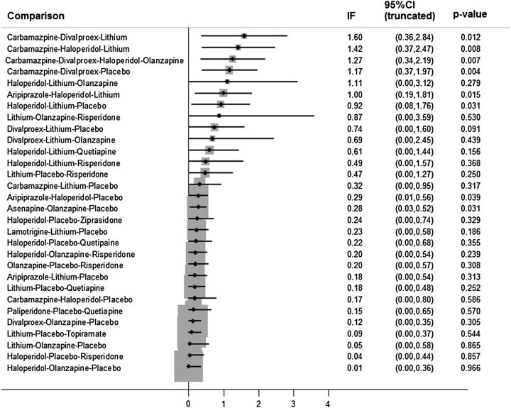
Consistency is a key assumption for NMA and should be checked in each closed loop of evidence. Figure 2 presents the inconsistency factors (differences between direct and indirect evidence) accompanied by the 95% CI and the p value from testing equality of direct and indirect evidence. We are not interested in the direction of inconsistency (if direct estimates exceed the indirect ones or vice versa), but only on the magnitude of inconsistency. Hence, we change direction of all negative inconsistency factors so that they can be depicted in a positive scale in a graph. A zero inconsistency factor implies that direct and indirect evidence are in agreement for that loop. Caution is needed because with many treatments and many closed loops of evidence we may find inconsistency in some loops by pure chance. In addition, it is common to have a few studies in some loops to compute the corresponding inconsistency factor with much certainty. Inconsistency cannot be excluded if inconsistency factors include zero but have wide 95% CIs. Large inconsistency may compromise the validity of results from a NMA. Several other methods have been suggested to test for inconsistency.^{20 25 26} If inconsistency is found, we may explore it using network metaregression²⁷ or encompass it by assuming statistical models that relax the consistency assumption.^{20 28} In figure 2 we see that there are significant inconsistencies in loops involving drugs such as carbamazepine, divalproex and lithium. These are drugs encountered in older studies. We found that the direct evidence from studies comparing carbamazepine and divalproex favoured divalproex (−0.84, 95% CI −1.63 to −0.03), while the indirect evidence favoured carbamazepine (0.30, 95% CI 0.01 to 0.57). Moreover, direct evidence for the relative effect for haloperidol versus lithium was very large (1.10, 95% CI 0.31 to 1.91) in favour of haloperidol whereas the indirect relative effect was very small (0.16, 95% CI 0.00 to 0.33).

Figure 2.

Inconsistency plot for the outcome ‘mean change’. Inconsistency factors (IF) along with their 95% CIs and the corresponding p values for testing equality between direct and indirect evidence are displayed. IFs are calculated as the absolute difference between direct and indirect estimates, and therefore CIs are truncated to zero. Loops of which the lower CI limit does not reach the zero line are considered to present statistically significant inconsistency.

Ranking of interventions

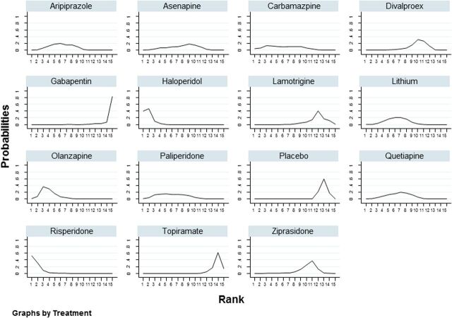
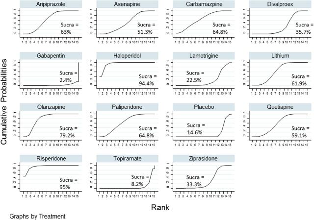
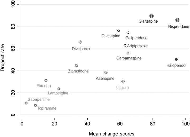
One of the unique features of a NMA is to rank the competing interventions. We can, for each treatment, estimate the probability of it assuming any of the possible ranks. It is common to use the ‘probability of being the best’ as a method of finding the best treatment. We strongly suggest against this practice because it does not take into account the uncertainty of the relative effect estimate and the probabilities of assuming any of the other possible ranks.²⁹ One can alternatively use rankograms and cumulative ranking probability plots.^{21 29} A rankogram plots the probabilities for treatment to assume any of the possible ranks. Figure 3 shows rankograms of the antimanic drugs for efficacy. Risperidone and haloperidol have high probabilities of being either best or second best drugs. Both drugs have probabilities larger than 80% of being among the two most effective drugs. This is also evident from figure 4, where we give the SUCRA value to each intervention, which is the ratio of the area under the cumulative ranking curve to the entire area in the plot. The more quickly the cumulative ranking curve approaches one, the more close to unity this ratio is. SUCRA values may be seen as the percentage of effectiveness (or safety) a treatment achieves in relation to an imaginary treatment that is always the best without any uncertainty. Ideally, we would like to see peaks in a rankogram or a steep increase in the cumulative ranking plot as that would suggest that the corresponding rank where we observe the peak is the most probable one for the antipsychotic. In our example, this happens for the most effective drugs (risperidone, haloperidol and olanzapine) and for least effective drugs (divalproex, gabapentin, lamotrigine, placebo, topiramate and ziprasidone). A similar distribution of rank probabilities across all (or many) possible ranks indicates uncertain ranking for that treatment. Figure 5 plots a scatterplot between the SUCRA values for efficacy and tolerability of antimanic drugs. We use different symbols to cluster drugs into groups. It seems that haloperidol makes a group on its own: although it is very effective, there are more patient dropouts from its trials than in trials of other effective drugs.

Figure 3.

Rankograms for the efficacy outcome.

Figure 4.

Cumulative ranking probability plots for the efficacy outcome. The SUCRA value for each intervention is given.

Figure 5.

Clustered ranking plot for efficacy and acceptability. Cluster techniques (single linkage clustering) were used to cluster interventions in groups defined by different symbols.

Comparison-adjusted funnel plot

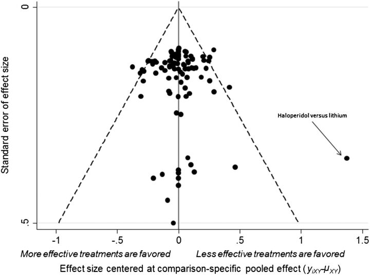
A funnel plot is a scatterplot between study effect size versus its inverted SE, and an asymmetrical funnel plot implies there are differences in effectiveness between small and large studies, also known as small-study effects.³⁰ With many treatments, there is not one summary estimate but many. Chaimani et al²¹ extended the use of the funnel plot to NMA by plotting the difference between the study-specific effect sizes from the corresponding comparison-specific summary versus the inverted SE. Prior to drawing this plot, it is important to order the treatments in a meaningful way, regarding which treatment the small-study effect would favour in a comparison. In figure 6 we sorted drugs according to efficacy as measured by their SUCRA values; in other words, our assumption was that more effective drugs were favoured in small trials. There was no asymmetry in the plot, suggesting that smaller studies do not favour more effective (or less effective) treatments. This plot may reveal outlying effect sizes for a given study size. For instance, in this working example we found a large effect size for a small study comparing haloperidol versus lithium. This big effect size may be responsible for large inconsistency factors observed in loops including this comparison.

Figure 6.

Comparison-adjusted funnel plot for efficacy.

Conclusions

There is a series of conceptual challenges when conducting a NMA and these should be borne in mind by clinicians who read such publications in scientific journals. First of all, disagreement between direct and indirect evidence (inconsistency) poses a threat to the validity of results from a NMA. Presentation of results is not as straightforward as in traditional meta-analysis. Forest plots are of little use in a NMA. Instead, relative effects may be presented in a league table and small-study effects can be explored by a comparison-adjusted funnel plot. NMA is a relatively new technique and methodology is advancing rapidly. There is a lot of ongoing research on how to evaluate the quality of evidence from a NMA. Until recently, NMA was understood by researchers with a strong statistical background but development of user-friendly software has acquainted clinicians to NMA and popularised the method. New methods for testing and accounting for inconsistency, and for ranking the available treatments are constantly being developed. Just as in traditional meta-analysis, publication bias³⁰ and missing outcome data³¹ which are very common in mental health trials may compromise overall results.

References

- 1.Centre for Evidence Based Medicine. Levels of evidence. 2015. http://www.cebm.net
- 2.Leucht S, Corves C, Arbter D, et al. Second-generation versus first-generation antipsychotic drugs for schizophrenia: a meta-analysis. Lancet 2009;373: 31–41. 10.1016/S0140-6736(08)61764-X [DOI] [PubMed] [Google Scholar]
- 3.Caldwell DM, Ades AE, Higgins JP. Simultaneous comparison of multiple treatments: combining direct and indirect evidence. BMJ 2005;331:897–900. 10.1136/bmj.331.7521.897 [DOI] [PMC free article] [PubMed] [Google Scholar]
- 4.Lu G, Ades AE. Combination of direct and indirect evidence in mixed treatment comparisons. Stat Med 2004;23:3105–24. 10.1002/sim.1875 [DOI] [PubMed] [Google Scholar]
- 5.Salanti G, Higgins JPT, Ades AE, et al. Evaluation of networks of randomized trials. Stat Methods Med Res 2008;17:279–301. 10.1177/0962280207080643 [DOI] [PubMed] [Google Scholar]
- 6.Nikolakopoulou A, Chaimani A, Veroniki AA, et al. Characteristics of networks of interventions: a description of a database of 186 published networks. PLoS ONE 2014;9:e86754. 10.1371/journal.pone.0086754 [DOI] [PMC free article] [PubMed] [Google Scholar]
- 7.Cipriani A, Higgins JP, Geddes JR, et al. Conceptual and technical challenges in network meta-analysis. Ann Intern Med 2013;159:130–7. 10.7326/0003-4819-159-2-201307160-00008 [DOI] [PubMed] [Google Scholar]
- 8.Salanti G. Indirect and mixed-treatment comparison, network, or multiple-treatments meta-analysis: many names, many benefits, many concerns for the next generation evidence synthesis school. Res Synth Method 2012;3:80–97. 10.1002/jrsm.1037 [DOI] [PubMed] [Google Scholar]
- 9.Sullivan SM, Coyle D, Wells G. What guidance are researchers given on how to present network meta-analyses to end-users such as policymakers and clinicians? A systematic review. PLoS ONE 2014;9:e113277. [DOI] [PMC free article] [PubMed] [Google Scholar]
- 10.Caldwell DM. An overview of conducting systematic reviews with network meta-analysis. Syst Rev 2014;3:109. 10.1186/2046-4053-3-109 [DOI] [PMC free article] [PubMed] [Google Scholar]
- 11.Cipriani A, Furukawa TA, Salanti G, et al. Comparative efficacy and acceptability of 12 new-generation antidepressants: a multiple-treatments meta-analysis. Lancet 2009;373:746–58. 10.1016/S0140-6736(09)60046-5 [DOI] [PubMed] [Google Scholar]
- 12.Cipriani A, Barbui C, Salanti G, et al. Comparative efficacy and acceptability of antimanic drugs in acute mania: a multiple-treatments meta-analysis. Lancet 2011;378:1306–15. 10.1016/S0140-6736(11)60873-8 [DOI] [PubMed] [Google Scholar]
- 13.Leucht S, Cipriani A, Spineli L, et al. Comparative efficacy and tolerability of 15 antipsychotic drugs in schizophrenia: a multiple-treatments meta-analysis. Lancet 2013;382:951–62. 10.1016/S0140-6736(13)60733-3 [DOI] [PubMed] [Google Scholar]
- 14.Mayo-Wilson E, Dias S, Mavranezouli I, et al. Psychological and pharmacological interventions for social anxiety disorder in adults: a systematic review and network meta-analysis. Lancet Psychiatry 2014;1:368–76. 10.1016/S2215-0366(14)70329-3 [DOI] [PMC free article] [PubMed] [Google Scholar]
- 15.Bucher HC, Guyatt GH, Griffith LE, et al. The results of direct and indirect treatment comparisons in meta-analysis of randomized controlled trials. J Clin Epidemiol 1997;50:683–91. 10.1016/S0895-4356(97)00049-8 [DOI] [PubMed] [Google Scholar]
- 16.Fournier JC, DeRubeis RJ, Hollon SD, et al. Antidepressant drug effects and depression severity: a patient-level meta-analysis. JAMA 2010;303:47–53. 10.1001/jama.2009.1943 [DOI] [PMC free article] [PubMed] [Google Scholar]
- 17.Chaimani A, Vasiliadis HS, Pandis N, et al. Effects of study precision and risk of bias in networks of interventions: a network meta-epidemiological study. Int J Epidemiol 2013;42:1120–31. 10.1093/ije/dyt074 [DOI] [PubMed] [Google Scholar]
- 18.Moher D, Pham B, Jones A, et al. Does quality of reports of randomised trials affect estimates of intervention efficacy reported in meta-analyses? Lancet 1998;352:609–13. 10.1016/S0140-6736(98)01085-X [DOI] [PubMed] [Google Scholar]
- 19.Stata Statistical Software [computer program]. Version version College Station TX: StataCorp LP, 2011.
- 20.White IR, Barrett JK, Jackson D, et al. Consistency and inconsistency in network meta-analysis: model estimation using multivariate meta-regression. Res Synth Methods 2012;3:111–25. 10.1002/jrsm.1045 [DOI] [PMC free article] [PubMed] [Google Scholar]
- 21.Chaimani A, Higgins JP, Mavridis D, et al. Graphical tools for network meta-analysis in STATA. PLoS ONE 2013;8:e76654. 10.1371/journal.pone.0076654 [DOI] [PMC free article] [PubMed] [Google Scholar]
- 22.Konig J, Krahn U, Binder H. Visualizing the flow of evidence in network meta-analysis and characterizing mixed treatment comparisons. Stat Med 2013;32:5414–29. 10.1002/sim.6001 [DOI] [PubMed] [Google Scholar]
- 23.Salanti G, Del GC, Chaimani A, et al. Evaluating the quality of evidence from a network meta-analysis. PLoS ONE 2014;9:e99682. 10.1371/journal.pone.0099682 [DOI] [PMC free article] [PubMed] [Google Scholar]
- 24.Puhan MA, Schunemann HJ, Murad MH, et al. A GRADE Working Group approach for rating the quality of treatment effect estimates from network meta-analysis. BMJ 2014;349:g5630. 10.1136/bmj.g5630 [DOI] [PubMed] [Google Scholar]
- 25.Dias S, Welton NJ, Caldwell DM, et al. Checking consistency in mixed treatment comparison meta-analysis. Stat Med 2010;29:932–44. 10.1002/sim.3767 [DOI] [PubMed] [Google Scholar]
- 26.Higgins JPT, Jackson D, Barrett JK, et al. Consistency and inconsistency in network meta-analysis: concepts and models for multi-arm studies. Res Synth Method 2012;3:98–110. 10.1002/jrsm.1044 [DOI] [PMC free article] [PubMed] [Google Scholar]
- 27.Cooper NJ, Sutton AJ, Morris D, et al. Addressing between-study heterogeneity and inconsistency in mixed treatment comparisons: application to stroke prevention treatments in individuals with non-rheumatic atrial fibrillation. Stat Med 2009;28:1861–81. 10.1002/sim.3594 [DOI] [PubMed] [Google Scholar]
- 28.Lu G, Ades AE. Assessing evidence inconsistency in mixed treatment comparisons. J Am Stat Assoc 2006;101:447–59. 10.1198/016214505000001302 [DOI] [Google Scholar]
- 29.Salanti G, Ades A, Ioannidis J. Graphical methods and numerical summaries for presenting results from multiple-treatment meta-analysis: an overview and tutorial. J Clin Epidemiol 2011;64:163–71. 10.1016/j.jclinepi.2010.03.016 [DOI] [PubMed] [Google Scholar]
- 30.Mavridis D, Salanti G. Exploring and accounting for publication bias in mental health: a brief overview of methods. Evid Based Ment Health 2014;17:11–15. 10.1136/eb-2013-101700 [DOI] [PubMed] [Google Scholar]
- 31.Mavridis D, Chaimani A, Efthimiou O, et al. Addressing missing outcome data in meta-analysis. Evid Based Ment Health 2014;17:85–9. 10.1136/eb-2014-101900 [DOI] [PubMed] [Google Scholar]