Abstract
Human-induced force analysis plays an important role across a wide range of disciplines, including biomechanics, sport engineering, health monitoring or structural engineering. Specifically, this paper focuses on the replication of ground reaction forces (GRF) generated by humans during movement. They can provide critical information about human-mechanics and be used to optimize athletic performance, prevent and rehabilitate injuries and assess structural vibrations in engineering applications. It is presented an experimental approach that uses an electrodynamic shaker (APS 400) to replicate GRFs generated by humans during movement, with a high degree of accuracy. Successful force reconstruction implies a high fidelity in signal reproduction with the electrodynamic shaker, which leads to an inverse problem, where a reference signal must be replicated with a nonlinear and non-invertible system. The solution presented in this paper relies on the development of an iterative neural network and an inversion-free approach, which aims to generate the most effective drive signal that minimizes the error between the experimental force signal exerted by the shaker and the reference. After the optimization process, the weights of the neural network are updated to make the shaker behave as desired, achieving excellent results in both time and frequency domains.
Keywords: Forces reconstruction, Human-induced forces, Artificial neural networks, Electrodynamic shaker, Ground reaction forces
1. Introduction
Human-induced force measurement and analysis play an increasingly important role in a wide spectrum of health-related disciplines such as biomechanics [1], [2], sport engineering [3], [4], [5] or health monitoring [6], [7]. In biomechanics, human-induced forces are often measured using a variety of technologies such as force plates, strain gauges or accelerometers [8]. Analysis of these forces can provide insight into the mechanics of human movement, such as joint moments and muscle forces. Specifically, Ground Reaction Forces (GRF), which are generated by the interaction between a foot and the ground, provide information about the mechanics of human movement, including stride length, step frequency and gait symmetry [9]. Temporal replication of ground reaction forces is crucial for understanding human locomotion, optimizing athletic performance, and developing technologies for injury prevention and rehabilitation [10], [11], [12].
In addition, in the field of structural engineering, the human-induced forces have great relevance. In this case, both acceleration and force signals are used for the assessment of vehicle [13] and aircraft vibrations [14]. Moreover, they are used for the analysis of Human-Structure Interaction (HSI) [15], [16]. In this context, human occupants can influence the dynamic properties (mass, stiffness, and damping) of slender structures [17], [18]. If the effects are not accounted in the design phase, they may cause: 1) structural damage, 2) a reduction in the lifespan of the structures, and 3) serviceability problems affecting the safety and comfort of its occupants. Although there are several established methods suitable for simulating human actions on slender structures through the combination of active and passive components [19], [20], the focus of this paper lies on physically reproducing forces equivalent to those exerted by a human using a non-human device. In [21] it was reported that the movements of an individual or a group of people could not be precisely duplicated in repeated experiments, even when a timing device was used. This is due to the fact that, when walking on a vibrating surface, pedestrians tend to modify their walking pattern to maximize their comfort. In addition, human walking characteristics are affected by a large number of factors, some associated with the subject defined as inter-subject (different people generate different loads), and others associated with individual subjects, defined as intra-subject (nobody makes two identical steps) [22], [23]. Consequently, this lack of repeatability in the tests makes the task of predicting structural vibrational response highly complex.
The experimental approach addressed in this work is based on the use of an electrodynamic shaker to reproduce the GRFs generated by humans. The shaker comprises an inertia-based actuator, which generates structural forces through the inertial movement of a mass. In the proposed framework, the shaker receives as an input a ±5 V signal, and its mass oscillates accordingly. Due to this operating method, it is not needed to use an explicit mathematical model of the walking force pattern, since the force time series, measured with instrumented insoles, is directly replicated. By accurately reproducing GRFs, researchers and engineers can develop effective strategies to mitigate the effects of vibrations on structures and vehicles, improve safety and comfort, and extend the lifespan of these assets; besides providing support for the understanding of human locomotion and for the development of technologies for injury prevention and rehabilitation. This approach involves measuring the forces generated by humans during various activities, such as bouncing and walking, and then replicating those forces using the electrodynamic shaker. Nonetheless, accurately replicating human-generated forces presents several challenges, including the non-linearity and ill-posedness of the problem. Despite these challenges, the replication of human forces with electrodynamic shakers holds great promise for advancing our understanding of the effects of human-generated vibrations on structures and materials.
Hence, this paper deals with the development of an offline algorithm capable of achieving high-precision signal reproduction with the electrodynamic shaker, which is a nonlinear electro-mechanical system [24]. The problem of inferring a system input belongs to a wide class of ill-posed inverse problems [25], and arises in different fields and applications, such as metrology, image processing or spectroscopy. Several strategies for dealing with this type of problem can be found in the literature: a high number of research related to adaptive control has been developed for shaking tables with the aim of simulating earthquakes and this has shown the important capabilities of the adaptive tuning of such complex systems [26], [27], [28], [29], [30], [31]. Adaptive control techniques for human-induced forces have been also explored in the field of humanoid robots [32], [33], [34]. An alternative approach involves the implementation of an iterative learning control system (ILC) [35], which is a control method that identifies the actuator model and iteratively modifies the drive signal. As we are dealing with a non-invertible model of the shaker dynamics, the problem becomes more difficult, leading to a highly non-trivial task. Solutions to this problem in the literature include the adoption of a more traditional approach to obtain the inverse model of the system based on classical inversion [36], [37], or using an alternative inversion method such as stable inversion [38] or adjoint systems [39], [40]. Also, approaches concerning modeling-free inversion-based iterative feed-forward control can be found in [41], as well as robust ILC designs with experimental verification [42], [43], [44]. Another alternative present in literature is the implementation of a model-based control similar to the one implemented in [27] for Multi-Axis Hydraulic Shaker. Lately, there has been a growing trend wherein model inversion is no longer required by using data-driven techniques [45], [46], [55], [48], [49]. In this context, Artificial Neural Networks (ANNs) have been intensively studied over the last few decades and are an appealing and flexible alternative to the classical control methods, as they can deal with nonlinear problems [50]. Neural networks have already been successfully employed in iterative frameworks applied to nonlinear systems [51], [52], [53], [54], [47].
Following this trend, a Machine Learning (ML) data-driven approach has been chosen to be applied in this paper. Therefore, a black box system based on an iterative neural network algorithm has been developed, verifying the stability and reliability of the method both by simulations and via experimental. The framework implemented consists of applying an ANN as a regressor to iteratively generate a drive signal. As the direct model of the shaker has been satisfactorily obtained in previous works [56], the error between the simulated shaker force and the reference is assessed at each iteration by simulation of the model. Consequently, the system selects the drive signals which produce an inertial force that is within a defined error tolerance compared to the reference, using these selected data to retrain the ANN in the next iteration. This process updates the ANN weights at each iteration, resulting in the drive signal converging towards an optimized value, as shown through experimentation. Because the network is exclusively trained using data from the shaker's ideal operational span, its output will be confined within this range, guaranteeing stable system operation.
The key contributions of this paper are outlined as follows: first, a methodology to accurately replicate human-generated forces with a mechanic actuator is presented. Second, a precursory method for systematizing dynamic load tests on structures has been reported, ensuring the process is completely objective, repeatable, and independent of pedestrian influence. Third, an offline algorithm employing ML techniques has been implemented on an electrodynamic shaker, eliminating the need for its inverse model, which constitutes a novelty in the field. Experimental tests have confirmed the system's optimal performance, convergence, and stability.
The manuscript is organized as follows. In Section 2, the procedure and description of the methods used in the experimental GRF data acquisition are set out. The dynamic behavior of the electrodynamic shaker and its modeling are presented in Section 3. The ANN design process and its implementation in the iterative algorithm are described in Section 4. The experimental validation of the proposed method is proposed in Section 5. Lastly, the discussion, conclusions, and suggestions for future work are presented in Section 6.
2. Experimental GRF data acquisition
The acquisition of experimental force data for subsequent replication is conducted utilizing a set of wireless instrumented insoles, recently released by Novel Gmbh (Munich, Germany) [57], [58]. The Loadsol© sensor, depicted in Fig. 1, is engineered to directly measure the total GRF normal to both the shoe and the plantar surface of the foot. Employing a sensor based on capacitors, highly ergonomic and linearly sensitive, spanning the entire plantar area, Loadsol© ensures that force is measured in a direction perpendicular to the plantar surface, regardless of its point of application. The sensor is affixed to a compact electronics unit attached onto the lateral or upper side of the footwear. Force data are captured at 100 Hz and transmitted wirelessly in real-time via Bluetooth to a smart device for storage, review, and analysis. The performance of this device has already been assessed in [59], [60].
Figure 1.
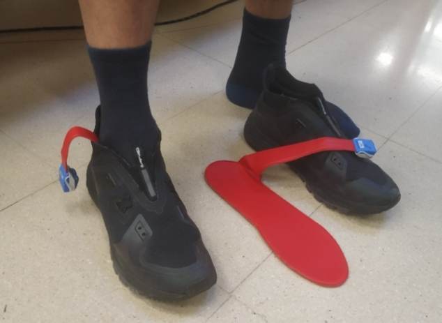
Loadsol sensorized insoles photography.
A total of 16 experimental force measurements are performed for different movement conditions at different frequencies and amplitudes (see Table 1), focusing motion types in which there is always at least one foot touching the ground (bouncing, walking, random excitation), to ease the replication of these signals using the electrodynamic shaker. Note that two kinds of random excitation are considered: one performed while keeping both feet on the ground and the other including movement at a random and non-constant pace. They differ from bouncing and walking in an attempt to create more complex and arbitrary signals in which the frequency content is unpredictable to ensure that the developed control system is capable of correctly dealing with such complex scenarios. Given that the shaker can solely exert forces at a single point, it was decided to replicate the sum of the forces associated to each foot, corresponding to the total force applied by the pedestrian on the ground. Measurements were conducted over a 20-second interval by a male individual standing at a height of 192 cm and weighing 77 kg.
Table 1.
Experimental force measurements.
| Name | Motion type | Frequency (Hz) | Amplitude |
|---|---|---|---|
| Exp 1 | Bouncing | 1 | Low |
| Exp 2 | Bouncing | 1 | High |
| Exp 3 | Bouncing | 1.5 | Low |
| Exp 4 | Bouncing | 1.5 | High |
| Exp 5 | Bouncing | 2 | Low |
| Exp 6 | Bouncing | 2 | High |
| Exp 7 | Bouncing | 2.5 | Low |
| Exp 8 | Bouncing | 2.5 | High |
| Exp 9 | Walking | 1.5 | - |
| Exp 10 | Walking | 1.75 | - |
| Exp 11 | Walking | 2 | - |
| Exp 12 | Walking | 2.25 | - |
| Exp 13 | Static random | - | Low |
| Exp 14 | Static random | - | High |
| Exp 15 | In motion random | - | Low |
| Exp 16 | In motion random | - | High |
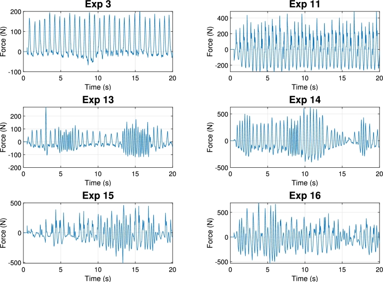
The signals recorded are loaded into MATLAB and undergo preprocessing, which involves combining the signals from both feet by summation, applying an offset to make the signal centered at 0 N and resampling the resulting force signal to 1000 Hz, which will be the input of the iterative ANN algorithm. Six of these reference force signals are displayed in Fig. 2. Note that after centering these signal around 0 N some of the force values become negative. The rationale behind this is that the focus of the study lies in the dynamics of the structure subjected to the applied force. Therefore, the static component of the force is eliminated by removing the offset, as the goal is that the shaker reproduces only the dynamic load centered at 0 N.
Figure 2.
Experimental reference force signals measured with Loadsol insoles.
3. Inertial-electrodynamic-mass actuator dynamics and modeling
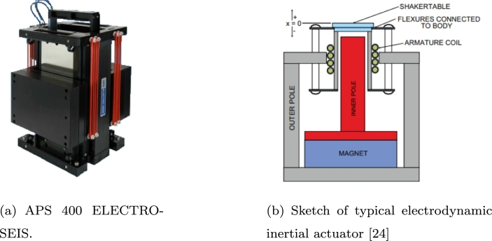
An inertial mass electrodynamic shaker was used for GRF replication, the specific model being an APS 400 ELECTRO-SEIS (Fig. 3(a)). These devices are commonly employed to induce forces in structures while undertaking dynamic tests. They generally operate by applying either a noise signal to the structure or a sinusoidal signal. The actuator consists of a moving reaction mass (denoted as ) attached to a current coil that moves in a magnetic field created by an array of permanent magnets. The moving mass is connected to the frame by a suspension system that can be modeled as a spring stiffness and a viscous damping (Fig. 3(b)). The shaker is powered by means of an amplifier which receives an electrical signal varying between ±5 V and provides the shaker with the necessary power signal in order for the moving mass to oscillate accordingly.
Figure 3.
Inertial electrodynamic mass actuator. (a) Picture of the model APS400, (b) Conceptual parts and components.
Further information about the different operational modes of these devices can be consulted at [61]. Voltage mode amplification has been used for force reconstruction, since it is the preferable choice for burst random and sine chirp excitation. The dynamics of an inertial mass actuator operating in voltage mode can be described as a third order transfer function relating the generated force F and the voltage input V as shown in Eq. (1) [56], where corresponds to the transducer constant (in N/A), is the natural frequency associated with the suspended moving mass system, represents the damping coefficient and the pole at ε accounts for the low-pass filtering property of these instruments, absorbing frequencies higher than the cut-off frequency ε (in rad/s).
| (1) |
The process of obtaining the model consists in optimizing the parameters of the transfer function by applying a curve-fitting algorithm so that the error between the experimental and analytical Frequency Response Function (FRF) is minimum. This task is undertaken through the lsqnonlin function implemented in MATLAB. The experimental FRF is calculated by applying a 60000-point Blackman window over the experimental data obtained by applying white noise as the input voltage signal V to the shaker in the range of with a test duration of 10 minutes and a sampling frequency of 1000 Hz. Experimental acceleration was measured with piezoelectric accelerometers (IEPE) from MMF (Metra Mess und Frequenztechnik), so an estimation of the applied force can be computed by multiplying the measured force by the value of the moving mass (31,2 kg). The amplifier's manual gain position is adjusted to 25% of its maximum capacity. The resulting parameter values are: rad/s (2.39 Hz), N/V, , and rad/s (9.89 Hz). Fig. 4 illustrates a comparison between the experimental and fitted FRF. It's important to note that the slight fluctuations observed in the experimental FRF magnitude at frequencies close to 0 Hz stem from the accelerometer's measurement range, which initiates at 0.16 Hz.
Figure 4.
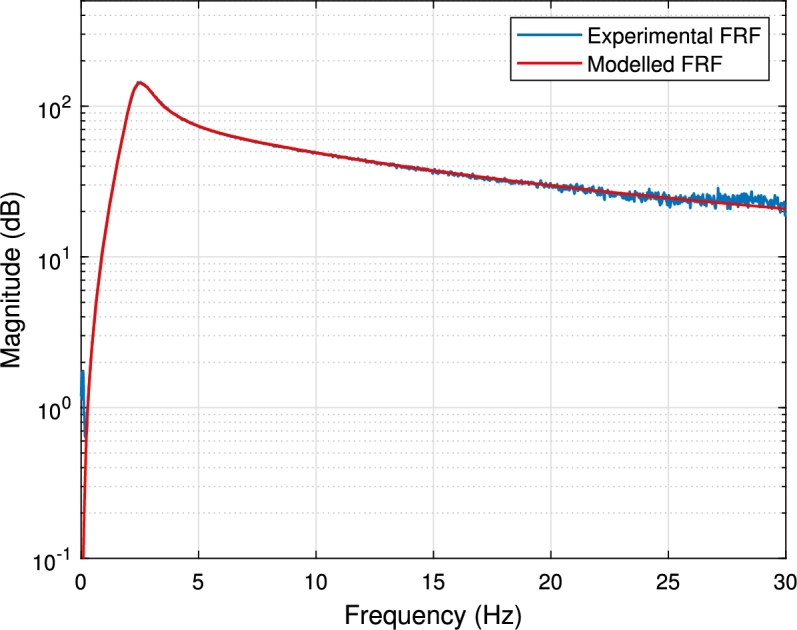
Actuator's transfer function, denoted by GA(s), whose magnitude is expressed in dB relative to 1 N/V.
4. Iterative neural network algorithm
This section describes the proposed methodology for addressing the GRF reconstruction. To ensure that the shaker generates a specific force, it must be supplied with the appropriate command signal V(t). Nonetheless, the generation of this signal is not a trivial process. Therefore, the framework implemented consists of applying an ANN as a regressor to iteratively generate a drive signal; the error between the simulated shaker force and the reference is assessed at each iteration by simulation of the shaker model. Consequently, the system selects the drive signals which produce an inertial force that is within a defined error tolerance compared to the reference, using these selected data to retrain the ANN in the next iteration.
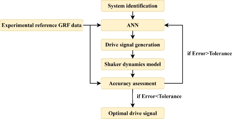
The basic flow diagram of the proposed iterative algorithm is shown in Fig. 5. First, the system identification is performed in order to obtain the actuator direct model. With this information, and with the desired reference signal as an input, the ANN retrieves an offline drive signal in each iteration. This signal is then applied to the actuator model and the simulated output signal is compared with the reference signal to evaluate the error in that iteration. If the error is greater than a defined tolerance, the algorithm is rerun, obtaining a new drive signal with the information acquired in the previous iteration. This procedure is repeated until an optimal simulated signal is obtained or until the maximum number of iterations is reached.
Figure 5.
Operation scheme of the proposed iterative control system.
In this framework, the ANN is responsible for providing a drive signal when the reference is inputted. This ANN is only altered at the end of an iteration, when the training data is updated and the network is retrained, keeping the original network structure intact (only the weights and biases are modified). In this scenario, the ANN operates as a regressor whose output is always bounded within the optimum operating voltage range of the actuator, as the ANN is only trained with data belonging to this range. The stability, reliability and convergence of the proposed method are verified by simulations. An explanation of the developed algorithm is presented in the following sections, starting with the ANN design process.
4.1. ANN design
ANN are adaptive systems that have been successfully used for solving a wide variety of problems that cover high levels of nonlinearity. Among the many possible ANN architectures, a single layer Multilayer Perceptron (MLP) has been employed. Regarding the selected ANN structure, the use of more sophisticated networks, such as recurrent networks (RNN) or Long short-term memory (LSTM), which take into account temporal data sequences, was considered. Nevertheless, it was noticed that, by implementing a simpler structure, such as the MLP with a single hidden layer, satisfactory results were obtained, so the simplest system was preferred as it allowed faster training and easier implementation. The theoretical fundamentals of this type of systems can be consulted in [62]. Since MLP neural networks behave as a universal approximator, the use of a single hidden layer is usually sufficient to guarantee the convergence of any regression problem. Moreover, it should be noted the lack of a unified criterion in the literature that helps to select the optimal value of layers or neurons per layer; instead these parameters are usually determined empirically. In this work, after some tests, the network was defined with three layers, including an input layer, a hidden layer and an output layer. Finally, the Resilient Backpropagation Algorithm [63] was employed to train the ANN. The remaining parameters established in the creation of the ANN can be consulted in Table 2.
Table 2.
Implemented ANN parameters.
| ANN Parameter | Value |
|---|---|
| Training ratio | 70% |
| Validation ratio | 15% |
| Test ratio | 15% |
| Training function | Resilient Backpropagation |
| Perform function | MSE |
| Limit training epochs | 10000 |
| Limit training time | 30000 |
| Training goal | 0.01 |
| Training minimum step | 1e-6 |
| Training maximum fails | 500 |
| Training minimum gradient | 1e-100 |
| Activation/Transfer function | Log-sigmoid |
The ANN design process consists in defining the inputs that the system needs in order to predict the voltage value required at each instant. Since an inertial shaker is used for that task, the force generated at a certain instant i is dependent not only on the voltage signal at the previous instant i-1, but also on the conditions of the moving mass (position and velocity) at that instant i-1, which is commonly known as its state. Furthermore, the limited range of movement of the moving mass (± 8 cm from its balance position) makes it necessary to predict the required movements of the moving mass sufficiently in advance in order to be able to reproduce the reference signal with the smallest possible global error. Hence, to determine the value of the voltage signal at instant i, it is necessary to feed the network with the desired reference signal data corresponding to the instants from i to i+m, where m is a parameter to be fixed in the algorithm. By doing this, the error between the reference and the output force at instant i would be greater if only the value of was taken into account. However, the overall error in the entire time signal will be significantly smaller and the stability of the system will be guaranteed.
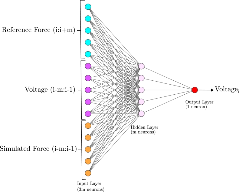
Consequently, after trying different combinations, the ANN is designed with the following structure (Fig. 6, where for legibility purposes). The initial m entries offer the ANN details regarding the anticipated future actions, while the remaining inputs supply information about the shaker's past state, including both voltage and generated force. After analyzing different values of m, the final algorithm has been designed with a value of , which corresponds to half a second of information. Therefore, the number of neurons in the input layer is equal to , the number of neurons in the hidden layer is , and the number of neurons in the output layer is 1, corresponding to the voltage value at instant i.
Figure 6.
Implemented ANN structure.
4.2. Iterative algorithm structure
Once the ANN structure and its design has been defined, this network is implemented in the iterative algorithm, as shown in Table 3.
Table 3.
Implemented ILC-ANN based algorithm.
| Iterative ANN algorithm |
|---|
| System identification |
| Reference signal preprocessing |
| Initialize |
| Initialize |
| Initialize |
| Initial data training generation |
| while < It limitdo |
| Train ANN |
| Optimal Reference offset selection |
| Drive signal generation |
| New training data selection |
| Iteration assessment |
| Update |
| Update |
| Update |
| end |
After identifying the system for determining its associated model (Section 3) and preprocessing the reference data, as commented in Section 2, the terminating variables of the algorithm are initialized and the initial training data of the ANN is generated (Fig. 7). At the beginning, the network is trained using noisy data and ramps spanning from the maximum to the minimum voltage, resulting in a voltage data buffer that is updated iteratively. This process ensures that the network is trained with progressively specific data. This buffer is limited to a maximum of k points (k=50000) to avoid an excessive training time of the ANN.
Figure 7.
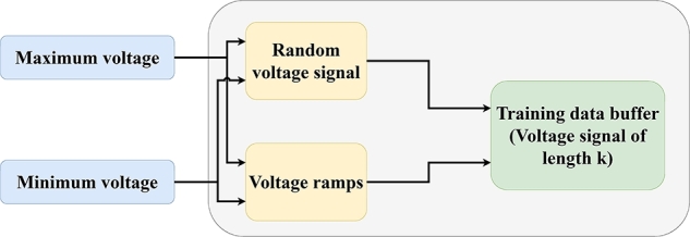
Initial training data generation.
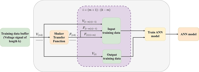
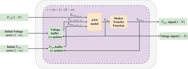
Using this voltage data buffer and the shaker transfer function, the input and output training data of the ANN are generated as shown in Fig. 8. The network is then trained with the previously defined network parameters (Table 2). Subsequently, this trained ANN is used to generate the iteration drive signal (Fig. 9). For this purpose, the reference signal is used as an input and the voltage and simulated force signals are initialized with m zeros (as well as the signal, which is set to start and finish with m zeros, in order to replicate the whole signal, since the algorithm needs this amount of initial and final points to work properly). As the signals are non-symmetrical and irregular over time, the process performance is highly sensitive to the offset in the reference signal, which means that this offset will determine whether or not the shaker is able to accurately follow the desired signals. For this reason, this drive generation process is repeated p times (with p defined as 5 to avoid increasing the iteration time excessively), in such a way that in each repetition the offset is set to a random value between ±10 N of the previous iteration offset value. Then, the errors committed between the simulated and reference force for each p repetition are compared and the optimal iteration offset value is selected and updated.
Figure 8.
ANN training.
Figure 9.
Drive signal generation.
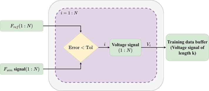
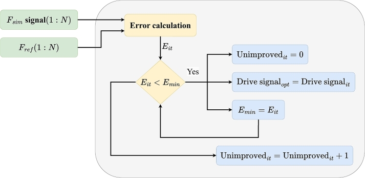
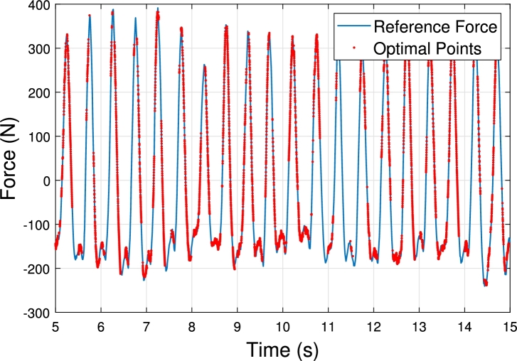
Afterwards, the simulation-generated force is compared with the reference in the time domain, and those points whose error is less than the defined tolerance are selected and the corresponding voltage points are appended to the training data buffer (Fig. 10). Finally, the error committed in that iteration is assessed to see whether or not it is lower than the minimum error obtained in the execution of the algorithm, being the terminating variables updated accordingly (Fig. 11). The RMSE (root-mean-square-error) (Eq. (2)) indicator between the simulated force signal and the reference signal is used as a criterion for assessing the iteration. Also, the number of data points selected in one iteration for the training of the following iterations is defined as the Optimal Points Ratio (OPR), which represents the percentage of points that are within the defined error tolerance with regard to the total number of points in the signal. An example of the OPR is illustrated in Fig. 12.
Figure 10.
Voltage training buffer update.
Figure 11.
Iteration assessment.
Figure 12.
Optimal Points Ratio.
| (2) |
The previously detailed algorithm is implemented through a Matlab R2020a script, which lets the user define parameters required by the algorithm (training voltage buffer length (k), ANN neurons, number of points for each input (m), maximum voltage, error tolerance, and maximum number of iterations), along with the specification of both the shaker dynamics model and the file (.txt) containing the force signal to be replicated, obtained from the Loadsol® app. The ANN is created using the parameters specified in Table 2 and by means of the feedforwardnetwork function of Deep Learning Toolbox.
5. Experiments and results
This section describes the experimental validation process. First, Section 5.1 is devoted to show how the methodology's performance is assessed in a simulated environment by comparing the reference signals with those provided by the shaker model when excited with the voltage signal proposed by the algorithm. Then, drive voltage signals are fed to the shaker for experimental validation of the methodology. Details on the experimental setup along with the results obtained are given in Section 5.2. Finally, Section 5.3 provides a discussion of the results obtained.
5.1. Simulation results
The developed algorithm is executed with the 16 reference signals described in Section 2. Since it consists of an offline system, the Matlab script with the implemented algorithm is launched by entering the Loadsol® files and the shaker dynamics model as inputs.
The parameters used for this execution are shown in Table 4.
Table 4.
Implemented algorithm parameters.
| Parameter | Value |
|---|---|
| Number of layers | 1 |
| Neurons per layer | 500 |
| Maximum voltage [V] | 3.7 |
| Training data buffer length (k) | 50000 |
| Number of points for each input (m) | 500 |
| Assessment criteria | RMSE |
| Error tolerance [N] | 10 |
| Number of maximum iterations | 7 |
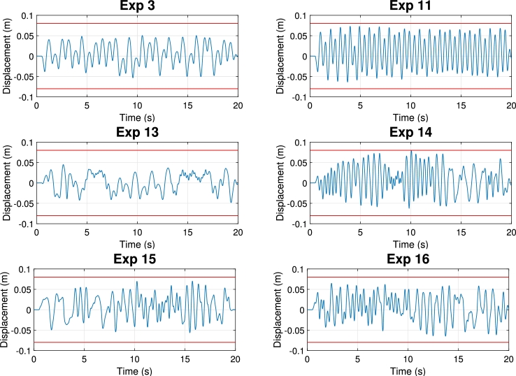
The maximum voltage value is established through the computation of the displacement of the moving mass. This calculation involves integrating the simulated acceleration signal, derived from modeling the system using the drive signal as input, twice. Consequently, a maximum voltage is selected to ensure that the moving mass remains within the constrained displacement range of the shaker (±8 cm), thereby preventing collisions between the moving mass and the end of the stroke limits. Fig. 13 illustrates the graph of simulated displacement for the shaker moving mass for 8 of the experiments, where it can be seen that, in all cases, the shaker moving mass does not reach the end-of-stroke limits (represented by two horizontal red lines).
Figure 13.
Expected displacement of the moving mass.
Table 5 presents the outcomes of the algorithm's execution, displaying the RMSE, OPR, and the number of iteration at which the best solution is achieved for each experiment. To guarantee the consistency of the outcomes and acknowledge the heuristic characteristics of the training algorithm, the experiments are repeated 10 times, with the tables showing the averaged values. It can be seen how the average number of iterations corresponds to 7.34 and the average RMSE corresponds to a value of 62.72 N. In addition, the simulated output of the iterative ANN algorithm in relation to the reference signal for the 10 depicted experiments is shown in Fig. 14, where it can be visually appreciated how the signals obtained resemble the reference signals in an remarkable way for all of the experiments at any time.
Table 5.
Experimental force measurements.
|
|
||||||||||||||||||||||||||||||||||||||||||||||||||||||||||||||||||||||||||||||||||||||||
Figure 14.
Simulated force signals (red) compared to the reference force signals (blue).
5.1.1. Error assessment metrics
The accuracy of the force replication procedure carried out for the 16 experimental signals can be assessed using 3 metrics [26]: root-mean-square (RMS) error r (Eq. (3)), time-domain error e (Eq. (4)) and correlation coefficient c (Eq. (5)).
| (3) |
| (4) |
| (5) |
where is the desired time signal, is the simulated force signal after inputting the optimum drive signal to the shaker model, rms stands for RMS, max is the maximum value, Cov denotes the covariance and D the variance.
The RMS error r describes the difference in energy between two signals. It reflects the error of the energy transmitted from the reference and the replicated force to the ground. It is usually used to judge the control accuracy and whether the offline iteration converges to tolerance. It is common that 0-0.2 is chosen as the convergence criterion [26].
The time-domain error e describes the comprehensive error level caused by the amplitude and time delay [26]. It is the average of the error percentage at each time point of the two signals, which has a relative value compared with the maximum peak value. The closer to zero the error is, the smaller the deviation between the two signals. It is well recognized that when the error is between 0 and 0.35 [64], the difference between the two signals can be considered to be very small.
The correlation coefficient c is a statistical indicator to describe the similarity between two signals. The closer to 1 the correlation coefficient is, the more similar the two signals are. It is generally believed that two signals are highly correlated when the correlation coefficient falls between 0.8 and 1 [65].
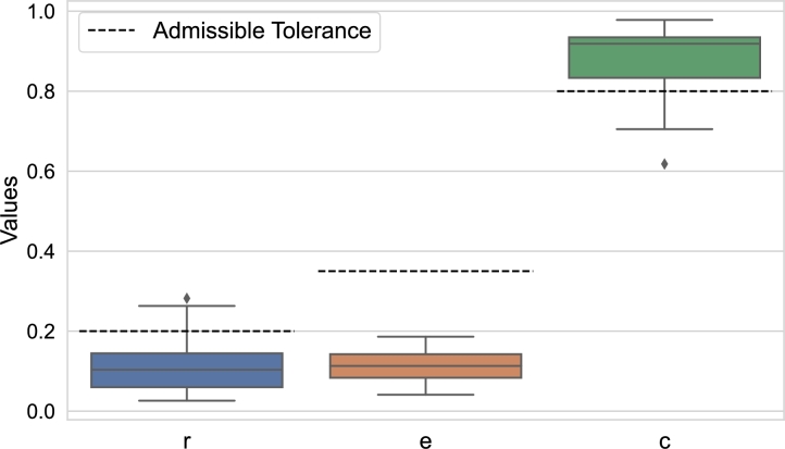
Table 6 shows the error indexes obtained for the simulated output signals regarding the 16 reference signals together with their corresponding mean and standard deviation (Std) values. Also, Fig. 15 shows the distribution of error metrics across the validation experiments. It can be noted that the averages of the 3 indexes for the set of performed experiments are within the admissible tolerance (0-0.2 for r, 0-0.35 for e and 0.8-1 for c). Only experiments 1 and 9 exhibit error indexes clearly outside these acceptance values, with correlation coefficients under 0.75. The signals from experiments 4 and 16 also present error indexes slightly outside the limits of acceptability. However, these instances arise because the reference force signals surpass the operational bounds of ± 400 N for the electrodynamic shaker. Consequently, the algorithm endeavors to attain the maximum achievable force without the moving mass of the shaker colliding with the end-of-stroke limits.
Table 6.
Error assessment indexes.
|
|
||||||||||||||||||||||||||||||||||||||||||||||||||||||||||||||||||||||||||||||||||||||||
Figure 15.
Distribution of error assessment metrics.
5.1.2. Convergence
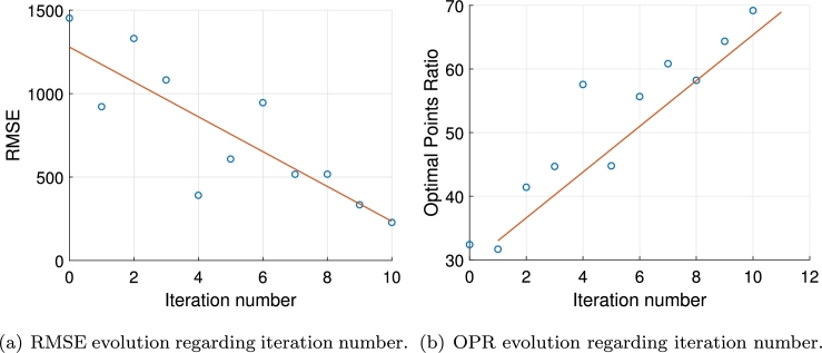
In order to analyze the algorithm convergence to an optimal output signal, the RMSE and OPR are compared to the number of iterations in each experiment with the aim of observing how they evolve with each iteration. Fig. 16 provides an example of the evolution of these indexes with regard to the number of iterations for experiment 13. It may be observed that this evolution can be depicted by a descending straight line in the case of RMSE (Fig. 16(a)) and by an ascending straight line for OPR (Fig. 16(b)). The slopes of these lines for each algorithm execution are reported in Table 7, noting that the average rate of improvement of the algorithm is 37.58 N per iteration. The only criterion used to determine if an iteration is better than the previous one is the RMSE, which explains why the slope of the OPR for experiments 1 and 4 is negative, since it is possible that an iteration presents a worse OPR than in previous iterations, but a better RMSE.
Figure 16.
Convergence analysis of the algorithm. (a) RMSE, (b) OPR.
Table 7.
Convergence analysis values.
| Exp | It. number | RMSE slope (N/it) | OPR slope (%/it) |
|---|---|---|---|
| Exp 1 | 1.4 | -41.11 | -6.48 |
| Exp 2 | 4.9 | -40.96 | 1.52 |
| Exp 3 | 9.5 | -35.56 | 3.62 |
| Exp 4 | 4.5 | -92.55 | -0.39 |
| Exp 5 | 3.6 | -13.45 | 3.42 |
| Exp 6 | 18.2 | -25.52 | 1.54 |
| Exp 7 | 5.5 | -29.05 | 2.49 |
| Exp 8 | 7.3 | -32.44 | 2.53 |
| Exp 9 | 4.2 | -50.45 | 3.66 |
| Exp 10 | 10.4 | -33.20 | 0.67 |
| Exp 11 | 10.4 | -15.14 | 0.15 |
| Exp 12 | 3.2 | -41.47 | 0.92 |
| Exp 13 | 11.5 | -10.99 | 3.33 |
| Exp 14 | 2.6 | -48.70 | 1.71 |
| Exp 15 | 11.0 | -51.11 | 1.23 |
| Exp 16 | 9.2 | -39.62 | 0.58 |
| Mean | 7.34 | -37.58 | 1.28 |
5.2. Experimental validation
Once the optimum drive signals have been obtained for each one of the 16 experiments, these signals are fed to the electrodynamic shaker, and the experimental output force is compared to the reference GRFs registered with the insoles.
5.2.1. Experimental set-up
In order to perform these experiments, the electrodynamic shaker was placed on a rigid floor in a laboratory atmosphere. The experimental output force (GRF) is determined through the measurement of the shaker's moving mass acceleration using a piezoelectric accelerometer. Subsequently, this acceleration is multiplied by the mass of the moving component (31.2 kg) to obtain the GRF. The configuration of the shaker was the same as described in Section 3, operating in voltage mode, with a maximum manual gain amplitude of 25% and with the same mass and damping configuration, ensuring that the model used to obtain the optimum voltage signals faithfully represents the real system.
5.2.2. Experimental results
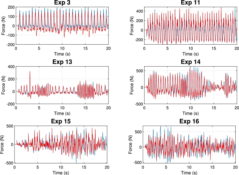
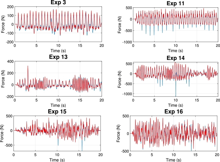
The experimental GRF signals obtained are shown in Fig. 17 compared to the simulated ones. It can be observed that the errors between both signals are minimal. Table 8 indicates the correlation coefficients between both signals for the 16 experiments, observing that all of them are above 0.94. Therefore, it is possible to conclude that the shaker direct model employed is highly precise, since the experimental signals correspond accurately to the simulated ones.
Figure 17.
Temporal comparison of the experimental force signal (blue) with regard to the simulated signal (red) for 6 of the experiments.
Table 8.
Correlation coefficients between experimental and simulated force signals.
|
|
||||||||||||||||||||||||||||||||||||||||||||
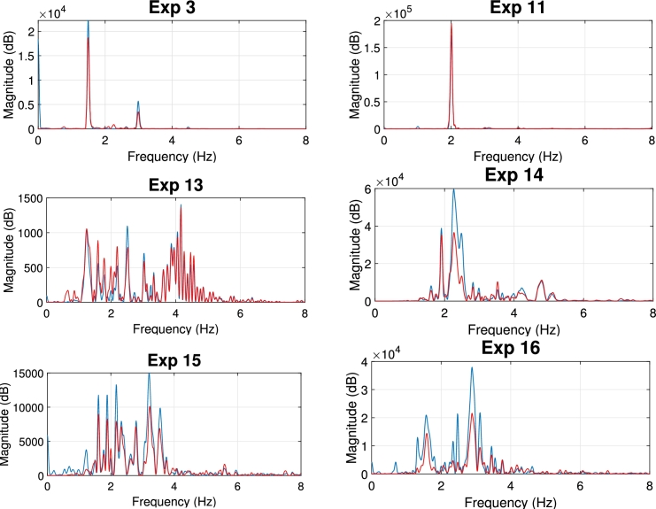
Furthermore, the experimental signals obtained are juxtaposed with the reference force in the frequency domain (Fig. 18). This comparison reveals that the frequency content of both signals remains relatively similar across all cases, albeit minor variations in amplitudes.
Figure 18.
Comparison in the frequency domain: Human signals (blue) as reference and their reproduction with the shaker (red).
As a result, when replicating these signals using the shaker on a flexible structure, similar frequencies will be excited as with forces exerted by a human individual. Consequently, the response of the structure will be alike in both cases.
5.3. Discussion
Once the experimental results have been presented, they are discussed in detail as follows. Regarding the performance of the algorithm for the different types of movements, it can be noted, from Table 6, that both bouncing (Exp 1-8) and walking (Exp 9-12) are replicated with higher fidelity in high frequencies (2, 2.5 Hz), while correlation coefficients for lower frequencies (1, 1.5 Hz) are slightly worse yet within the admissible tolerances. This phenomenon can be understood by examining the shaker FRF in Fig. 4. It shows that the system's amplitude is significantly lower at lower frequencies compared to near its natural frequency (2.39 Hz), indicating a reduced ability to generate forces at those frequencies, which illustrates that the efficiency of the system will always be limited to the employed equipment. It is also noteworthy that significant differences exist in the performance obtained for the static and in motion random signals, with rather worse error indexes for the latter. However, it is important to emphasize that all these error indexes are within the acceptable tolerance range (except Exp 9 whose c is slightly out), and Fig. 14 illustrates how the time domain signal replication is very satisfactory.
When observing the frequency content of the reproduced force signals compared to the referenced (Fig. 18), minor differences are found in terms of frequency components, with practically all the frequencies of the reference signals represented in the experimentally obtained. Discrepancies in replicating time domain signals manifest in the frequency domain as slight variations in amplitudes.
In any case, the results presented in this paper reveal the good performance of the iterative control system developed, achieving an optimal and satisfactory efficiency in both the time and frequency domains, as can be seen in the Figure 14, Figure 17, Figure 18, and evidenced by the error rates within the acceptable tolerance ranges. This will allow to perform dynamic tests to assess serviceability automatically and without the need for skilled workers, ensuring that dynamic response of the structure will be similar to the application of forces by a human subject.
6. Conclusions
An iterative neural network algorithm has been developed to solve the inverse control problem of an electrodynamic shaker, achieving a reliable reproduction of the ground reaction forces produced by different types, amplitudes and frequencies of human motion or locomotion activities. A total of 16 experiments have been developed to compare the simulated signals with the reference ones. The comparison has been developed in time domain, but also evaluating the frequency content of the signals.
The proposed implementation is based on a iterative Artificial Neural Network (ANN) approach, aiming at solving the ill-posed inverse problem of inferring a system input from a specific reference. Also, since dealing with a highly non-trivial task as the shaker dynamics are modeled with a non-invertible model, an alternative to the classical control has been proposed and validated consisting of reproducing the behavior of the inverse model of the electrodynamic shaker by the ANN. This offers a solution without the need for inversion and assures the system's stability. The experimental work shows that, for the 16 cases, excellent results are obtained for all the evaluated metrics. Also, being an iterative algorithm, its convergence is studied, revealing an average rate of decrease of the RMSE is 37.58 N per iteration, which indicates the progressive learning that the model undertakes.
The high-precision replication at any time of the force signal, with the nonlinear electrodynamic shaker, (within its operating range) represents a significant step in the area of study. It has a high interest in a wide variety of disciplines. In addition, it leads to the following future lines of research in the field of structural engineering: (1) it will be possible to perform serviceability tests on structures in a repeatable way and without requiring skilled people. Therefore, the effects of the different human actions (walking, bouncing, etc.) on the structures can be assessed in a reliable and repeatable way. (2) With the goal of reproducing not only static human actions but also dynamic locomotive movements, the electrodynamic shaker will be equipped with movement capabilities across the structure. (3) Observing and learning from the differences between the structure's response when excited by the shaker and by a pedestrian will facilitate the analysis of human-structure interaction phenomena through a purely experimental perspective. (4) By introducing multiple shakers it will be possible to study the effects caused by groups of several synchronized or unsynchronized pedestrians.
Ethics statement
The study did not require ethical approval.
CRediT authorship contribution statement
César Peláez-Rodríguez: Writing – original draft, Software, Methodology, Investigation, Conceptualization. Álvaro Magdaleno: Writing – original draft, Visualization, Methodology, Conceptualization. José María García Terán: Resources, Formal analysis, Conceptualization. Jorge Pérez-Aracil: Writing – review & editing, Visualization, Supervision, Software. Sancho Salcedo-Sanz: Writing – review & editing, Validation, Project administration. Antolín Lorenzana: Writing – review & editing, Validation, Project administration, Funding acquisition.
Declaration of Competing Interest
The authors declare that they have no known competing financial interests or personal relationships that could have appeared to influence the work reported in this paper.
Acknowledgements
The authors wish to acknowledge to the AEI, Spanish Government (10.13039/501100011033) and to “ERDF A way of making Europe”, for the partial support through the grant PID2022-140117NB-I00. This research has also been partially supported by the project PID2020-115454GB-C21 of the Spanish Ministry of Science and Innovation (MICINN).
Contributor Information
César Peláez-Rodríguez, Email: cesar.pelaez@uah.es, cesar.pelaez@alumnos.uva.es.
Álvaro Magdaleno, Email: alvaro.magdaleno@uva.es.
José María García Terán, Email: teran@uva.es.
Jorge Pérez-Aracil, Email: jorge.perezarazil@uah.es.
Sancho Salcedo-Sanz, Email: sancho.salcedo@uah.es.
Antolín Lorenzana, Email: ali@eii.uva.es.
References
- 1.Lu T., Chang C. Biomechanics of human movement and its clinical applications. Kaohsiung J. Med. Sci. 2012;28:S13–S25. doi: 10.1016/j.kjms.2011.08.004. [DOI] [PubMed] [Google Scholar]
- 2.Ezati M., Ghannadi B., McPhee J. A review of simulation methods for human movement dynamics with emphasis on gait. Multibody Syst. Dyn. 2019;47:265–292. [Google Scholar]
- 3.Jaen-Carrillo D., Garcia-Pinillos F., Carton-Llorente A., Almenar-Arasanz A., Bustillo-Pelayo J., Roche-Seruendo L. Test–retest reliability of the OptoGait system for the analysis of spatiotemporal running gait parameters and lower body stiffness in healthy adults. Proc. Inst. Mech. Eng., Part P: J. Sports Eng. Technol. 2020;234:154–161. [Google Scholar]
- 4.Garcia-Pinillos F., Chicano-Gutierrez J., Ruiz-Malagon E., Roche-Seruendo L. Influence of RunScribe™ placement on the accuracy of spatiotemporal gait characteristics during running. Proc. Inst. Mech. Eng., Part P: J. Sports Eng. Technol. 2020;234:11–18. [Google Scholar]
- 5.Gao Z., Mei Q., Xiang L., Baker J., Fernandez J., Gu Y. Effects of limb dominance on the symmetrical distribution of plantar loading during walking and running. Proc. Inst. Mech. Eng., Part P: J. Sports Eng. Technol. 2022;236:17–23. [Google Scholar]
- 6.Liu X., Zhao C., Zheng B., Guo Q., Duan X., Wulamu A., Zhang D. Wearable devices for gait analysis in intelligent healthcare. Front. Comput. Sci. 2021;3 [Google Scholar]
- 7.Preeti M., Guha K., Baishnab K., Dusarlapudi K., Raju K. Low frequency MEMS accelerometers in health monitoring–a review based on material and design aspects. Mater. Today Proc. 2019;18:2152–2157. [Google Scholar]
- 8.Goss L., Crafton J., Davis B., McMillan G., Berki V., Howe A., Papp M. Plantar pressure and shear measurement using surface stress-sensitive film. Meas. Sci. Technol. 2019;31 [Google Scholar]
- 9.Alaqtash M., Yu H., Brower R., Abdelgawad A., Sarkodie-Gyan T. Application of wearable sensors for human gait analysis using fuzzy computational algorithm. Eng. Appl. Artif. Intell. 2011;24:1018–1025. [Google Scholar]
- 10.Johnson C., Tenforde A., Outerleys J., Reilly J., Davis I. Impact-related ground reaction forces are more strongly associated with some running injuries than others. Am. J. Sports Med. 2020;48:3072–3080. doi: 10.1177/0363546520950731. [DOI] [PubMed] [Google Scholar]
- 11.Jafarnezhadgero A., Fatollahi A., Amirzadeh N., Siahkouhian M., Granacher U. Ground reaction forces and muscle activity while walking on sand versus stable ground in individuals with pronated feet compared with healthy controls. PLoS ONE. 2019;14 doi: 10.1371/journal.pone.0223219. [DOI] [PMC free article] [PubMed] [Google Scholar]
- 12.Harry J., Blinch J., Barker L., Krzyszkowski J., Chowning L. Low-pass filter effects on metrics of countermovement vertical jump performance. J. Strength Cond. Res. 2022;36:1459–1467. doi: 10.1519/JSC.0000000000003611. [DOI] [PubMed] [Google Scholar]
- 13.Reichel K., Meywerk M. A MIMO system for the replication of accelerations excited in a vehicle by single obstacle crossings at comfort-relevant excitation points in a comfort simulator. J. Vibroeng. 2023;25 [Google Scholar]
- 14.Mauersberger M., Hähnel F., Wolf K., Markmiller J., Knorr A., Krumm D., Odenwald S. Predicting ground reaction forces of human gait using a simple bipedal spring-mass model. R. Soc. Open Sci. 2022;9 doi: 10.1098/rsos.211582. [DOI] [PMC free article] [PubMed] [Google Scholar]
- 15.Camacho-Gómez C., Wang X., Pereira E., Díaz I., Salcedo-Sanz S. Active vibration control design using the Coral Reefs Optimization with Substrate Layer algorithm. Eng. Struct. 2018;157:14–26. [Google Scholar]
- 16.Pacini B., Kuether R., Roettgen D. Shaker-structure interaction modeling and analysis for nonlinear force appropriation testing. Mech. Syst. Signal Process. 2022;162 [Google Scholar]
- 17.Shahabpoor E., Pavic A., Racic V. Interaction between walking humans and structures in vertical direction: a literature review. Shock Vib. 2016;2016 [Google Scholar]
- 18.Sachse R., Pavic A., Reynolds P. Human-structure dynamic interaction in civil engineering dynamics: a literature review. Shock Vib. Dig. 2003;35:3–18. [Google Scholar]
- 19.Živanović S. Modelling human actions on lightweight structures: experimental and numerical developments. MATEC Web Conf. 2015;24 [Google Scholar]
- 20.Lucà F., Berardengo M., Manzoni S., Vanali M., Drago L. Human-structure interaction: convolution-based estimation of human-induced vibrations using experimental data. Mech. Syst. Signal Process. 2022;167 [Google Scholar]
- 21.Tuan C., Saul W.E. Loads due to spectator movements. J. Struct. Eng. 1985;111(2):418–434. [Google Scholar]
- 22.Shahabpoor E., Pavic A. Topics on the Dynamics of Civil Structures, vol. 1. 2012. Comparative evaluation of current pedestrian traffic models on structures; pp. 41–52. [Google Scholar]
- 23.Ruiz D., Magluta C., Roitman N. Experimental verification of biomechanical model of bipedal walking to simulate vertical loads induced by humans. Mech. Syst. Signal Process. 2022;167 [Google Scholar]
- 24.Abhishek S., Tiwari N. Modeling and study of nonlinear effects in electrodynamic shakers. Mech. Syst. Signal Process. 2017;85:162–176. [Google Scholar]
- 25.Bakushinsky A., Goncharsky A. Ill-posed problems: theory and applications. Math. Appl. 1994;301 [Google Scholar]
- 26.Guo W., Shao P., Li H., Long Y., Mao J. Accuracy assessment of shake table device on strong earthquake output. Adv. Civ. Eng. 2019 [Google Scholar]
- 27.Chen P., Chang C., Spencer B., Tsai K. Adaptive model-based tracking control for real-time hybrid simulation. Bull. Earthq. Eng. 2015 [Google Scholar]
- 28.Shen G., Lv G., Ye Z., Cong D., Han J. Implementation of electrohydraulic shaking table controllers with a combined adaptive inverse control and minimal control synthesis algorithm. IET Control Theory Appl. 2011;2011 [Google Scholar]
- 29.Yachun T., Peng P., Dongbin Z., Yi Z. A two-loop control method for shaking table tests combining model reference adaptive control and three-variable control. Built Environ. 2018 [Google Scholar]
- 30.Stoten D., Gómez E. Adaptive control of shaking tables using the minimal control synthesis algorithm. Philos. Trans. R. Soc., Math. Phys. Eng. Sci. 2001 [Google Scholar]
- 31.Wen J., Zhao C., Wang Y., Shi Z. Extended-state-observer-based adaptive robust control of a single-axis hydraulic shaking table. IET Control Theory Appl. 2024;18:442–453. [Google Scholar]
- 32.Barfi M., Karami H., Faridi F., Sohrabi Z., Hosseini M. Improving robotic hand control via adaptive Fuzzy-PI controller using classification of EMG signals. Heliyon. 2022;8 doi: 10.1016/j.heliyon.2022.e11931. [DOI] [PMC free article] [PubMed] [Google Scholar]
- 33.Vughuma J., Verlinden O. ICBBE '19: Proceedings of the 2019 6th International Conference on Biomedical and Bioinformatics Engineering. Association for Computing Machinery; 2019. Control algorithm for an active ankle-foot orthosis: adaptative admittance control; pp. 91–98. [Google Scholar]
- 34.Qi W., Fan H., Karimi H., Su H. An adaptive reinforcement learning-based multimodal data fusion framework for human–robot confrontation gaming. Neural Netw. 2023;164:489–496. doi: 10.1016/j.neunet.2023.04.043. [DOI] [PubMed] [Google Scholar]
- 35.Arimoto S., Kawamura S., Miyazaki F. Bettering pperation of robots by learning. J. Robot. Syst. 1984;1(2):123–140. [Google Scholar]
- 36.Widrow B., Bilello M. Proceedings of the 1993 IEEE International Symposium on Intelligent Control. 1993. Adaptive inverse control. [Google Scholar]
- 37.Silverman L. Inversion of multivariable linear systems. IEEE Trans. Autom. Control. 1969;14(3):270–276. [Google Scholar]
- 38.Devasia S., Chen D., Paden B. Nonlinear inversion-based output tracking. IEEE Trans. Autom. Control. 1996;41(7):930–942. [Google Scholar]
- 39.Sogo T., Kinoshita K., Adachi N. Proceedings of the 39th IEEE Conference on Decision and Control. vol. 4. 2000. Iterative learning control using adjoint systems for nonlinear non-minimum phase systems; pp. 3445–3446. [Google Scholar]
- 40.Kinosita K., Sogo T., Adachi N. Iterative learning control using adjoint systems and stable inversion. Asian J. Control. 2002;4 [Google Scholar]
- 41.Kim K., Zou Q. A modeling-free inversion-based iterative feedforward control for precision output tracking of linear time-invariant systems. IEEE/ASME Trans. Mechatron. 2012;18:1767–1777. [Google Scholar]
- 42.Tayebi A., Abdul S., Zaremba M., Ye Y. Robust iterative learning control design: application to a robot manipulator. IEEE/ASME Trans. Mechatron. 2008;13:608–613. [Google Scholar]
- 43.Xu J., Qu Z. Robust iterative learning control for a class of nonlinear systems. Automatica. 1998;34:983–988. [Google Scholar]
- 44.Meng D., Moore K. Robust iterative learning control for nonrepetitive uncertain systems. IEEE Trans. Autom. Control. 2016;62:907–913. [Google Scholar]
- 45.Meng D., Jia Y., Du J., Yu F. Data-driven control for relative degree systems via iterative learning. IEEE Trans. Neural Netw. 2011;22(12):2213–2225. doi: 10.1109/TNN.2011.2174378. [DOI] [PubMed] [Google Scholar]
- 46.Yu X., Hou Z., Polycarpou M., Duan L. Data-driven iterative learning control for nonlinear discrete-time MIMO systems. IEEE Trans. Neural Netw. Learn. Syst. 2021;32(3):1136–1148. doi: 10.1109/TNNLS.2020.2980588. [DOI] [PubMed] [Google Scholar]
- 47.Chen Y., Jiang W., Charalambous T. Machine learning based iterative learning control for non-repetitive time-varying systems. Int. J. Robust Nonlinear Control. 2023;33:4098–4116. [Google Scholar]
- 48.Liu W., Cheng L., Hou Z., Yu J., Tan M. An inversion-free predictive controller for piezoelectric actuators based on a dynamic linearized neural network model. IEEE/ASME Trans. Mechatron. 2015;21:214–226. [Google Scholar]
- 49.Zhang Y., Wu J., Huang P., Su C., Wang Y. Inverse dynamics modelling and tracking control of conical dielectric elastomer actuator based on GRU neural network. Eng. Appl. Artif. Intell. 2023;118 [Google Scholar]
- 50.Haykin S. 2nd edition. Prentice-Hall; New Jersey.: 1999. Neural Networks. A Comprehensive Foundation. [Google Scholar]
- 51.Patan K., Patan M. Neural-network-based iterative learning control of nonlinear systems. ISA Trans. 2020;98:445–453. doi: 10.1016/j.isatra.2019.08.044. [DOI] [PubMed] [Google Scholar]
- 52.Afsharnia F., Madady A., Menhaj M. Neural iterative learning identifier-based iterative learningcontroller for time-varying nonlinear systems. Asian J. Control. 2021:1–15. [Google Scholar]
- 53.Xu Q., Zhan C., Wei Y. 2018 IEEE Symposium on Product Compliance Engineering - Asia (ISPCE-CN) 2018. Neural network-based AILC for non-repetitive trajectory tracking of non-affine pure-feedback discrete-time systems; pp. 1–5. [Google Scholar]
- 54.Yu Y., Zhang C., Cao W., Huang X., Zhang X., Zhou M. Neural network based iterative learning control for magnetic shape memory alloy actuator with iteration-dependent uncertainties. Mech. Syst. Signal Process. 2023;187 [Google Scholar]
- 55.Chen Y., Jiang W., Charalambous T. Machine learning based iterative learning control for non-repetitive time-varying systems. Electr. Eng. Syst. Sci. 2021;2021 [Google Scholar]
- 56.Casado C., Díaz I., Sebastián J., Poncela A., Lorenzana A. Implementation of passive and active vibration control on an in-service footbridge. Struct. Control Health Monit. 2013;20:70–87. [Google Scholar]
- 57.Peebles A., Ford K., Taylor J., Hart J., Sands L., Queen R. Using force sensing insoles to predict kinetic knee symmetry during a stop jump. J. Biomech. 2019;95 doi: 10.1016/j.jbiomech.2019.07.037. [DOI] [PubMed] [Google Scholar]
- 58.Renner K., Blaise-Williams D., Queen R.M. The reliability and validity of the Loadsol® under various walking and running conditions. Sensors. 2019;19:265. doi: 10.3390/s19020265. [DOI] [PMC free article] [PubMed] [Google Scholar]
- 59.Seiberl W., Jensen E., Merker J., Leitel M., Schwirtz A. Accuracy and precision of loadsol® insole forcesensors for the quantification of ground reaction force-based biomechanical running parameters. Eur. J. Sport Sci. 2018;18(8):1100–1109. doi: 10.1080/17461391.2018.1477993. [DOI] [PubMed] [Google Scholar]
- 60.Burns G., Zendler J., Zernicke R. Validation of a wireless shoe insole for ground reaction force measurement. J. Sports Sci. 2018;37(10):1129–1138. doi: 10.1080/02640414.2018.1545515. [DOI] [PubMed] [Google Scholar]
- 61.Peres M., Bono R., Brown D.L. Proceedings of the ISMA. 2010. Practical aspects of shaker measurements for modal testing; pp. 2539–2550. [Google Scholar]
- 62.Principe J., Euliano N., Lefebvre W.C. John Wiley & Sons; 2020. Neural and Adaptive Systems: Fundamentals Through Simulations. [Google Scholar]
- 63.Günther F., Fritsch S. Neuralnet: training of neural networks. R J. 2010;2:30. [Google Scholar]
- 64.Guan G., Xiong W., Wang H., Han J. 2009 International Conference on Information Engineering and Computer Science. 2009. 6 Degree-0f-freedom long-term waveform replication control; pp. 1–4. [Google Scholar]
- 65.Zhang J.Y. Comparison of application of grey correlation degree and Pearson correlation coefficient. J. Chifeng Univ. (Nat. Sci. Ed.) 2014;21:1–2. [Google Scholar]


