Identifying highly-valued bank customers with current accounts based on the frequency and amount of transactions

Abstract

We hypothesize that highly-valued bank customers with current accounts can be identified by a high frequency of transactions in large amounts of money. To test our hypothesis, we employ machine learning predictive models to real data, including 407851 transactions of 4760 customers with current accounts in a local bank in Jordan. Thus, we exploit three clustering algorithms: density-based spatial clustering of applications with noise, spectral clustering, and ordering points to identify the clustering structure. The two segments of customers (generated from the clustering process) have different transactional characteristics. Our customer behavioral segmentation accuracy is, at best, 0.99 and at least 0.82. Likewise, we build three classification models using our segmented data: a neural network, a support vector machine, and a decision tree. Our predictive models have an accuracy of 0.97 at best and 0.90 at least. Our experimental results confirm that the frequency and amount of transactions of bank customers with current accounts are most likely sufficient indicators for recognizing those customers whom banks highly value. Our predictive models state that the two most critical indicators are the deposit and withdrawal transactions performed on ATMs. In contrast, the least significant indicators are the transactions of credit cards and credit cheques.

1. Introduction

Around ten percent of businesses' revenue was spent on marketing in 2022 (according to the annual survey conducted by Gartner Incorporation [29]). Industries, including banks, must adopt an effective marketing strategy that pays off. To this end, a business has to address the needs of its customers while identifying their differences. The significance of personalized marketing is evident in a study [13] that showed an increase of 5%–15% in revenue that was directly attributed to the successful implementation of personalization, with an improvement of 10%–30% in marketing efficiency within a single channel. This paper focuses on recognizing highly-valued bank customers with current accounts through their transactional behavior. We hypothesize that highly-valued customers are associated with a high frequency of transactions in large amounts of money. To test this hypothesis, we utilized machine learning methods to process real customer data in a local bank in Jordan. Identifying highly-valued customers is vital in enabling banks to characterize their customers so that the bank might be better able to set an effective marketing strategy that addresses every customer's needs and, eventually, the bank might decide better whether new services need to be launched or if some existing services need to be discontinued (or be enhanced). Thus, ultimately, the bank can increase the satisfaction level of its customers. Given that the experiments of this study are implemented in a local bank in Jordan, we shed some light on the banking sector in Jordan. The banking industry in Jordan is crucial to Jordan's economy. There are 23 Jordanian commercial banks. Jordan might be considered a modest economy with a Gross Domestic Product (GDP) of US 44 billion, whereas Jordan's population is around 11 million. Nonetheless, according to the Bank Assets to GDP Country rankings of the year 2020 [52], Jordan was ranked 20 among 142 countries. In 2020, it was estimated that the volume of combined assets in the Jordanian banking sector is around US$ 80 billion, which is the equivalent of 189% of Jordan's GDP [8].

We contribute in this paper by testing the hypothesis that highly-valued bank customers can be identified by the frequency and amount of their transactions with the bank. Thus, we employ machine learning methods for processing real data, including 407851 transactions of 4760 customers with current accounts in a local bank in Jordan. We call a bank account of a highly-valued customer special account, whereas we refer to the accounts of the rest of the bank's customers by standard accounts. Since the bank accounts of our data are not labeled special or standard, our first issue is segmenting the existing customers (included in our data) based on their transactional behavior into two types of accounts: standard and special. Thus, we implemented three standard clustering algorithms: density-based spatial clustering of applications with noise, spectral clustering, and ordering points to identify the clustering structure. The two segments of customers (generated from the clustering process) have different transactional characteristics. Our customer behavioral segmentation accuracy is, at best, 0.99 and at least 0.82. Our second issue is automating further the process of dynamically assigning customers to standard or special accounts based on their transactional behavior with the bank. Hence, we build three classification models using our segmented data: a neural network, a support vector machine, and a decision tree. Our predictive models have an accuracy of 0.97 at best and 0.90 at least. Therefore, our experiments confirmed that the frequency and amount of transactions of bank customers with current accounts are most likely sufficient indicators for recognizing those customers whom banks highly value. Our predictive models state that the two most critical indicators are the deposit and withdrawal transactions performed on ATMs. In contrast, the least significant indicators are the transactions of credit cards and credit cheques.

In section 2, we discuss related work. In section 3, we describe our data and methods. In section 4, we present and discuss our experimental results. In section 5, we conclude the paper and indicate further directions of this research.

2. Related work

Using machine learning methods in finance research is prevalent, for example [3], [45], [38], [39], [44]. Likewise, one finds numerous studies on behavioral analysis within the finance sector, see for example [37], [30], [36]. As our research reported in this paper aims (for the long run) at a more stable banking sector, there is extensive literature in this arena see for instance [34], [32], [7], [53], [55]. On the other hand, one can find tremendous work in the broad field of “customer segmentation” as a tool for understanding the needs and differences between the customers of a given business; see, for example, [41], [24], [18], [51], [25], [46], [33], [35], [4], [40], [31]. To our knowledge, we do not see in the literature any work that thoroughly addresses the particulars of our study. Nevertheless, we overview a sample of the most recent related studies that implement bank customer segmentation worldwide. In the literature (discussed below), the interested reader may find additional citations on related earlier customer-segmentation projects. The manuscript of [10] suggested an evolutionary approach to segmenting customers in a bank in North Africa based on their credit card transactions. The article of [9] presented a study on segmenting customers of a bank in the United Kingdom using two known methods: k-means and density-based spatial clustering of applications with noise (dbscan). The paper of [43] proposed an enhancement to the well-known “recency, frequency, and monetary” model by adding a fourth dimension, “adoption”, to the model and then applying the enhanced model with clustering to actual bank data in Egypt. The monograph of [27] used the k-means algorithm to segment customers' behavior in electronic and traditional banking in Iran. The paper of [11] demonstrated a study on classifying bank customers based on their transactions in Russia using the well-known long short-term memory network method. The monograph of [19] uses two well-known segmentation techniques, k-means, and fuzzy c-means, to divide customers based on their transactions in Turkey. The article of [20] applies the k-means method to separate customers of the United Bank of Africa. Lastly, we note that the work of [26] uses dbscan to cluster customers of a bank in Iran.

3. Data and methods

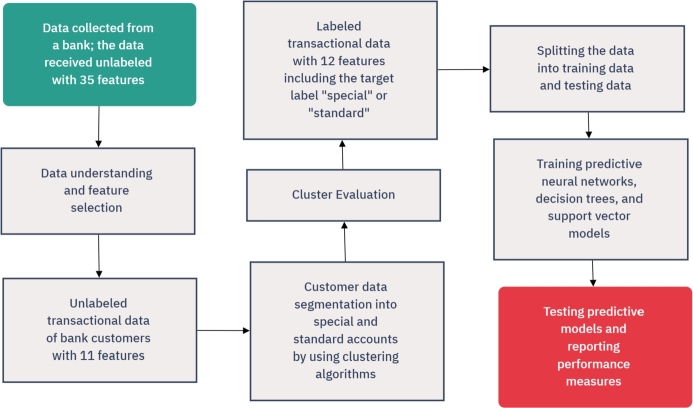
We describe our data features, preparation, and processing methods. Fig. 1 gives an overview of our methodology.

Figure 1.

Summary of our methodology.

3.1. Data acquisition and identification

A local bank in Jordan has provided us with a sample of customer data exclusively for this study. Upon their request, we do not reveal the identity of the collaborator bank. The received data includes genuine 407851 transactions of 4760 customers randomly selected from the bank's customers. All of the customers included in our data are individuals with current accounts. All of the transactions in our data occurred from 1 June 2021 to 30 June 2022. Table 1 shows the 35 features of the data received from the bank.

Table 1.

The features of our data.

#	Feature Name	Notes
1	Customer Number	made up for anonymity.
2	dob	birth date of the customer.
3	Gender	female or male.
4	City	the city of the customer's residency.
5	Country	the customer's country of residence.
6	Resident	“true” if the customer resides in Jordan.
7	Nationality	the citizenship of the customer.
8	Marital Status	married, single, divorced, or widowed.
9	Employer	the place of the customer's work.
10	Work Type	the customer's job description.
11	Business Line	the customer's job sector.
12	Position Title	the customer's job title.
13	Source of Income	the customer's source of income.
14	Monthly Income	the customer's monthly income.
15	pep	“true” if the customer is a politically exposed person.
16	fatca	“true” if the US Foreign Account Tax Compliance Act applies.
17	Risk Rate	“low”, “medium”, or “high”.
18	kyc	this stands for “know-your-customer”; it indicates whether a customer's account has been created.
19	Tier	Tier 1 to 4; a tier defines the cashback of credit or debit card purchases.
20	Housing Loan	“true” if the customer has a housing loan.
21	Personal Loan	“true” if the customer has a personal loan.
22	Auto Loan	“true” if the customer has a loan for financing a car purchase.
23	Credit Card	“true” if the customer holds a credit card.
24	Has Facility	“true” if the customer has a loan or a credit card.
25	Prepaid Card	“true” if the customer holds a prepaid card.
26	Receive Salary	“true” if the customer receives salary regularly.
27	Salary Amount	in Jordanian dinars representing the customer's salary amount.
28	Cashback Amount	the money rewarded to customers for credit or debit card purchases.
29	Has International Transfer	“true” if the customer send/receive money internationally.
30	Transaction Date	the date of a customer's transaction.
31	Transaction Amount	the customer's transaction amount.
32	Narrative	transactions' detail, e.g. the url of the shopping website.
33	Merchant Category	the business field of the merchant of the transaction.
34	Online_Offline	this indicates if the transaction is “online” or “offline”.
35	Transaction Type	cash deposit, atm withdrawal, atm deposit, bills, credit card, debit card, outward transfer, inward transfer, cash withdrawal, credit cheques, debit cheques.

Features 2–14 are filled out by the customer. Features 2–8 must be filled out and can be easily verified by the bank using a copy of the customer's identity card, passport, family book, or utility bill (water or electricity). Features (8–14) are optional and so can be missing. The bank fills the rest of the features, i.e., 15–35. Now, we will give further notes on features 15–35.

Feature 15 (i.e., pep) is a boolean value that indicates whether the customer is a politically exposed person (i.e., a person who has been assigned a significant public function). This feature is not missing in any record of our data. The bank may see that a customer is pep according to the discretion of the bank's employee, who may follow routine procedures such as requesting the customer for some information. However, our collaborator bank did not provide us with any specific process they usually follow to assess their customers concerning this feature.

Feature 16 (i.e., fatca) refers to the “Foreign Account Tax Compliance Act” of the United States, which requires foreign banks to verify if a customer is connected to the United States. This feature is not missing in any record of our data. The bank did not inform us about specific procedures for checking this feature. Still, the bank might rely on the information declared by the customer upon opening the bank account.

Feature 17, i.e., Risk Rate, estimates how suspicious the bank is about a customer account being connected to terrorism or laundering activities. This feature is not missing in any record of our data. The bank did not inform us about any specific procedure for evaluating customers concerning this feature. However, we observed an association between feature 17 (i.e., Risk Rate) and customer's nationality (feature 7), where around 70% of the customers with “Risk Rate = high” are not Jordanian, knowing that only 6% of the customers are not Jordanian. A justification might be that non-Jordanian customers can hardly provide the bank with supporting documents verifying their source of income.

Feature 18, “know your customer” (kyc), indicates whether a customer's account is created successfully, closed, or pending further verification by the bank side or inactive awaiting action from the customer side. This feature is not missing in any record of our data. However, 4745 customer accounts have this feature being “created”, whereas only 14 customers have a “pending” account status, and one customer record has a “closed” status.

Feature 19 (i.e., Tier) has four possible values: Tier 1, Tier 2, Tier 3, and Tier 4. This feature defines the percentage of cashback customers receive from credit card purchases, with Tier 1 being the account with the highest cashback percentage. The bank did not inform us about any specific procedure they follow in defining customers' tiers. An easy way to determine a tier for a given customer might be based on the opening balance of the customer's account. However, although difficult to implement manually, the quantity and quality of the customer's transactions over time might be more sensible to assign customer tiers dynamically. The bank did not state whether this feature is updated dynamically to reflect the actual status of the customer's account. Thus, whenever a customer transfers most of his balance to another bank, we are unsure if this customer is still assigned to the same tier. Likewise, when a considerable amount of money is deposited in the customer's account, we are uncertain if the customer is moved to a different tier.

Referring to Table 1, the bank fills features 20–25. So, they are reliable and entirely available (i.e., no missing values).

Concerning features 26–27, which the bank fills, note that for any customer record with “Receive Salary=false”, the “Salary Amount” value is left unspecified. Still, one can safely assume that the “Salary Amount” is 0 for any record that has “Receive Salary=false”.

Regarding feature 28 in Table 1, missing “Cashback Amount” in a record means the customer has received zero cashback.

Features 29–30, i.e., “has international transfer” and “transaction date”, are filled out by the bank, so they have no missing values in any record of our data.

Regarding feature 31 (i.e., Transaction Amount), our data includes 202 transactions with zero amounts. Some merchants perform such transactions to test that a customer's card is valid before accepting payments. Feature 31 has no missing value in any record of our data.

Feature 32 (i.e., Narrative) is missing in 26% of our data, feature 33 (i.e., Merchant Category) is missing in 59% of our data, and feature 34 (i.e., Online_Offline) is missing in half of the data; however, missing values of feature 34 can be easily inferred from feature 35 (i.e., Transaction Type), knowing that the value of feature 35 is missing in 31 transactions only.

In the next section, we describe the preparation of our data.

3.2. Data preparation

This section describes and justifies our feature selection and data preprocessing. As we discuss thoroughly in this section, many of the features mentioned in Table 1 in the previous section are not relevant to the aim of this study, which is to utilize customer transactional behavior to recognize those customers who are likely most valued to the bank. For example, demographic data such as age or gender are irrelevant to identifying highly-valued customers based on their transactional behavior. Additionally, another significant portion of the data is not accurate. Yet, many features have missing values in considerable amounts. For feature by feature, we elaborate intensively on our feature selection in the remainder of this section. Note that throughout this section, we refer to Table 1 whenever we mention our data features by bringing up their # number (listed in the first column of Table 1).

We dropped features 2–14 from the data. As noted before, some of these features are not required to be filled out for customers (namely features 8–14), so they are frequently missing. Most importantly, even if they are available, they are not verified or might not be kept up-to-date, so they are unreliable. Features 2–3 (date of birth and gender) are irrelevant to our study, which aims to identify different customer behaviors. Even if we want to include age and gender for customer segmentation, we might not be able to do so because, in several records of our data, the date-of-birth feature indicates that the account holder is underage. The guardians of those minor customers are probably the actual managers of such accounts. So, the behavior of such bank accounts will be connected to those guardians whose age or gender is unknown to us. Features 4–8 are not missing in any data record; the bank usually verifies them upon opening bank accounts. However, they might not be updated regularly. This is because such information, e.g., residency address, can change easily but might not be reflected in the data. Although the nationality (feature 7) might not change often, we did not consider it because around 94% of the customers (of our data) are Jordanian.

We did not consider feature 15, i.e., “personally exposed person” (pep). This feature is subject to the discretion of bank employees. Most importantly, only five customers are flagged with “pep=true” among the 4760 customers in our data.

Feature 16, i.e. fatca, is not helpful for our study. This boolean feature might be decided based on information provided by the customer. Such information might be incomplete or inaccurate. Most importantly, in our data, only seven customers have “fatca=true”.

Feature 17, i.e., Risk Rate, is irrelevant to our study, so it is dropped. This feature might help monitor accounts for illegal activities such as money laundering or terrorism. Moreover, this feature is just speculation by the bank rather than a definite determination based on tangible evidence.

Feature 18, i.e., kyc, is dropped as it will not help with the purpose of our study. Recall that 4745 out of 4760 customers are with “kyc=created”.

We dropped feature 19, i.e., Tier. This feature in our data is biased towards Tier 4 because most customers (3989 out of 4760) are in Tier 4, whereas 33 customers are in Tier 1, 77 are in Tier 2, and 661 are in Tier 3. So, it is hard to infer anything from this feature when most of our customers are in the same tier.

We dropped features 20–24 for two reasons. First, the distribution of these features is not balanced. For example, only nine customers have a housing loan (feature 20). For features 21–23, the number of customers with a specific financial facility is at most 170 out of the 4760 customers in our data. The second reason for dropping these features is that our data does not include further information about these loans: whether they are ongoing or paid in full, the loan standing amount, ... etc.

Feature 25, i.e., Prepaid Card, will not be considered further in our analysis. Our data does not indicate whether the customer has ever used a prepaid card because there are no prepaid card transactions in our data.

Features 26–27 (“Receive Salary” and “Salary Amount”) are based on information provided by the customer and not verified by the bank, which makes this feature unreliable. We observed numerous records in our data with salaries of less than 20 Jordanian dinars, which is too small to be true. So, we dropped features 26–27.

Regarding feature 28, i.e., cashback for each transaction, the feature is not used for two reasons. First, feature 28 is missing in around 68% of the data. Second, this feature does not help with the target of this paper, which is centered around classifying customers based on their behavior, where such a feature does not reflect an element of customer behavior.

We dropped feature 29. The bank tracks feature 29 (i.e., “has an international transfer” flag) for security reasons (such as monitoring for money laundering or terror activities). Feature 30 (i.e., transaction date) is not considered because we aim to analyze our data at the customer level, not the transaction level. For example, we do not mean to examine the transactions to identify specific patterns. Our primary aim is to classify customers based on their behavior.

We did not consider features 32–33 (i.e., Narrative and Merchant Category) because a considerable portion of the data is missing values for both features. Recall that 26% of our data is missing a value for feature 32 while 59% of the data is missing a value for feature 33. Most importantly, the content of feature 32 (i.e., the Narrative feature) is often unuseful. For example, in a record in our data, a narrative entry indicates the name of the person who deposited cash into the customer's account; in another, a narrative entry indicates the area name where the atm transaction occurs. Features 32–33 might be helpful for other purposes, such as tracking a customer's transactions for security issues. Still, they are irrelevant given the objectives of our study.

We dropped feature 34 (i.e., Online_Offline) because it is redundant; its value can be inferred from feature 35 (i.e., Transaction Type), which is kept for further analysis.

Therefore, we utilize two features for further analysis: features 31 and 35 (i.e., Transaction Amount and Transaction Type, respectively). As mentioned earlier, feature 35 is missing in thirty-one records only. So we dropped the records that have “Transaction Type” missing. However, after deleting such records, we still have 4760 customers in our data. Afterward, we created eleven new features from features 31 and 35. Recall that there are eleven transaction types: cash deposit, atm withdrawal, atm deposit, bills, credit card, debit card, outward transfer, inward transfer, cash withdrawal, credit cheques, and debit cheques. Likewise, recall that our data tracks the transactions performed by 4760 customers between 1 June 2021 and 30 June 2022. Thus, for each transaction type, we create a new feature x to hold (for some customer i) the total amount of all transactions of type x performed by customer i between 1 June 2021 and 30 June 2022. Consequently, our prepared data has 4760 records for 4760 distinct customers, where each record includes 11 fields: cash deposit, atm withdrawal, atm deposit, bills, credit card, debit card, outward transfer, inward transfer, cash withdrawal, credit cheques, and debit cheques. Our prepared data is a table of 4760 rows with 11 columns. For each row i (corresponding to customer i), a transaction-type field, x, of record i represents the total amount of money transacted as of type x by customer i between 1 June 2021 and 30 June 2022.

3.3. Data processing methods

This section gives a concise theoretical description of the methods we implemented in our experiments. Essentially, we clustered our customer data into two clusters using three methods: density-based spatial clustering of applications with noise (dbscan), spectral clustering (sc), and ordering points to identify the clustering structure (optics). Each generated cluster is considered a different class of customers; subsequently, each customer record (in our data) is given a label identifying the cluster to which the customer belongs. Then, we build three predictive models using the labeled data: a neural network, a support vector machine, and a decision tree.

We stress that employing clustering is critical in our study since the original customer data initially received from the bank was not labeled with “special account” or “standard account”. To test our research hypothesis, we build behavior-based predictive models identifying those special accounts from standard ones based on the transactional behavior of the account holder. We must train our predictive models with labeled data. Hence, clustering algorithms become very useful because they label our customers' unlabeled data with “special account” or “standard account”, enabling us to construct machine learning predictive models to classify future unlabeled customer accounts.

Density-based spatial clustering of applications with noise

Density-Based Spatial Clustering of Applications with Noise (dbscan) identifies clusters in a given data based on a distance function defined by the user of the algorithm [21]. We recall a description of dbscan from [21]. Let ϵ and φ be positive integers, and D be a set of d-dimensional points. The ϵ-neighborhood of a point $p\in D$, denoted by $N_{ϵ}(p)$, is defined by $N_{ϵ}(p)=\{q\in D|d(p,q)\le ϵ\}$ where $d(p,q)$ denotes a distance function between $p\in D$ and $q\in D$. Note that any appropriate distance function can be chosen for a given application. A point $p\in D$ is directly density-reachable from a point $q\in D$ with respect to ϵ and φ if $p\in N_{ϵ}(q)$ with $|N_{ϵ}(q)|\ge \phi$. A point p is density-reachable from a point q with respect to ϵ and φ if there is a chain of points $p_1,...,p_n$, $p_1=q$, $p_n=p$ such that $p_{i+1}$ is directly density-reachable from $p_i$. A point p is density-connected to a point q concerning ϵ and φ if there is a point o such that both p and q are density-reachable from o concerning ϵ and φ. A cluster C with respect to ϵ and φ is a non-empty subset of D satisfying the following conditions:

• •$\forall p,q\in D$: if $p\in C$ and q is density-reachable from p with respect to ϵ and φ, then $q\in C$.
• •$\forall p,q\in C$: p is density-connected to q with respect to ϵ and φ.

Let $C_1,...,C_k$ be the clusters of D with respect to parameters ${ϵ}_i$ and ${\phi }_i$, where $i=1,...,k$. Then $noise=\{p\in D|\forall i:p\notin C_i\}$.

Ordering points to identify the clustering structure

The following brief description of Ordering Points to Identify the Clustering Structure (optics) is borrowed from [49]. The optics algorithm can be seen as a generalization of dbscan that shifts the ϵ requirement from a single value to a value range. The main difference between dbscan and optics is that the optic algorithm constructs a reachability graph, which assigns each sample both a reachability distance and a spot within the cluster ordering; these two attributes are used to determine cluster membership. The cluster extraction with optics looks at the steep slopes within the reachability graph to find clusters, and the user of optics can define what counts as a steep slope. For a fuller presentation of the optics algorithm, we refer the reader to [5].

Spectral clustering

Spectral clustering is a well-known technique [54]. A spectral clustering algorithm includes the following actions [50]:

• 1.Get (as input) the data points $x_1,\dots ,x_n$ and the number, k, of clusters to construct.
• 2.Construct a similarity graph G = (V,E). Each vertex $v_i$ in this graph represents a data point $x_i$ and the weight on the edge connecting two nodes to be a given measure of the similarity between the two nodes.
• 3.Compute the unnormalized Laplacian L.
• 4.Compute the first k generalized eigenvectors $u_1,\dots ,u_k$ of the generalized eigenproblem $Lu=\lambda Du$.
• 5.Let $U\in {\mathbb{R}}^{n\times k}$ be the matrix containing the vectors $u_1,\dots ,u_k$ as columns.
• 6.For $i=1,\dots ,n$, let $y_i\in {\mathbb{R}}^k$ be the vector corresponding to the i-th row of U.
• 7.Cluster the points ${(y_i)}_{i=1,\dots ,n}$ in ${\mathbb{R}}^k$ with the k-means algorithm into clusters $C_1,\dots ,C_k$.
• 8.Output the clusters $A_1,\dots ,A_k$ with $A_i=\{j|y_j\in C_i\}$.

Support vector machines

Support Vector Machine (svm) is a supervised machine learning method. We recall the definition of (svms) from [12], [16]. Given training vectors ${\mathit{x}}_i\in {\mathbb{R}}^n$, $i=1,\dots ,l$, in two classes, and an indicator vector $\mathit{y}\in {\mathbb{R}}^l$ such that $y_i\in \{1,-1\}$. Then, svm estimates a decision function $sign({\mathit{w}}^T\varphi (\mathit{x})+b)$ by solving the optimization problem of (1).

$$\begin{gathered} \underset{\mathit{w},b,\mathit{\xi }}{\min }\frac{1}{2}{\mathit{w}}^T\mathit{w}+C\sum _{i=1}^l{\xi }_i \\ \mathrm{\text{subject to}}{y}_i({\mathit{w}}^T\varphi ({\mathit{x}}_i)+b)\ge 1-{\xi }_i,{\xi }_i\ge 0,i=1,\dots ,l, \end{gathered}$$ (1)

where $\varphi ({\mathit{x}}_i)$ maps ${\mathit{x}}_i$ into a higher-dimensional space and $C>0$ is the standardization parameter.

Decision trees

Decision Trees (dts) are a classical statistical method (see, for example, the monograph of [15]). dts are supervised machine learning used for classification. The goal is to create a tree that predicts the data class by learning simple decision rules derived from the data features. The tree's internal nodes represent data features, while the tree's leaf nodes denote target classes. The tree's branches emitting from an internal node designate the feature values corresponding to the node. A significant advantage of dts is that decisions made by dt models are explainable. There are several algorithms in the literature for building decision trees; see, for example, the survey of [17].

Neural networks

Neural Networks (nns) are a prevalent supervised machine learning method. nns were primarily proposed in the previous century [42], [47], and nowadays, they are a powerful technique with enormous modern applications in diverse fields. For binary classification problems, nns learn a function $f:{\mathbb{R}}^n\to \{0,1\}$ by training on a data set, where n is the number of dimensions for input, and the output is either 0 or 1. For a set of features $\{x_1,\dots ,x_n\}$ and a target $y\in \{0,1\}$, nns can learn a non-linear function approximator for binary classification problems. nns consists of several processing nodes (historically called neurons) organized in layers. The first layer of a nn is for the input values of the feature set, and the last layer is for the output that represents a prediction of the class variable. There can be one or more layers between the input and the output layer, called hidden layers. Given a set of m training examples $\{{\mathit{x}}_1,y_1\},\dots ,\{{\mathit{x}}_m,y_m\}$ where ${\mathit{x}}_i$ denotes the values of $x_1,\dots ,x_n$ for training example i and $y_i\in \{0,1\}$ is the class for training example i. A nn with one-neuron hidden layer learns the function $f(\mathit{x})=sigmoid(wg({\mathit{w}}^T\mathit{x}+b_1)+b_2)$ where $\mathit{w}\in {\mathbb{R}}^n$, $w,b_1,b_2\in \mathbb{R}$ are the model parameters, g is a nonlinear function, called the activation function. For further details on machine learning with nns, we refer the reader to [48], [6] for example.

3.4. Evaluation measures

We measured the accuracy score of our clusterings and classification models. Let ${\hat{y}}_i$ be the predicted class of the $i^{th}$ example and $y_i$ be the corresponding true class, and let n be the number of examples, then the accuracy score of a classifier is equal to $\frac{1}{n}{\sum }_{i=1}^n({\hat{y}}_i=y_i)$.

Further, we measured the standard scores of precision, recall, and F measure as defined next. Given n examples labeled with “positive” or “negative”, the precision of a classifier (concerning the positive label) is equal to the ratio of the number of examples classified as “positive” correctly over the number of all examples that are classified as “positive”; further, the recall of a classifier (concerning the positive label) is equal to the ratio of the number of examples that are classified as “positive” correctly over the number of examples that are indeed “positive”.

As a summarization metric combining precision and recall scores, F score is the harmonic mean of precision and recall, as equation (2) states.

$$Fscore=2\times \frac{precision\times recall}{precision+recall}$$ (2)

Likewise, we report on the standard score of the Receiver Operating Characteristic–Area Under Curve (ROC–AUC) that represents the estimated area under the ROC curve of the concerned classifier. An ROC curve plots the False Positive Rate (FPR) against the True Positive Rate (TPR). FPR and TPR are defined in equations (3) and (4).

$$TPR=\frac{TP}{TP+FN}$$ (3)

$$FPR=\frac{FP}{FP+TN}$$ (4)

Observe TP (FP, respectively) stands for the number of examples that are classified “positive” correctly (wrongly, respectively), and TN (FN, respectively) stands for the number of examples that are classified “negative” correctly (wrongly, respectively).

Lastly, for our classification models, we measured our features' importance by randomly permuting the values of a single feature and observing the effect of each shuffling on the model's accuracy [14].

4. Experimental results

We implemented1 our experiments using Python 3.9.7 and the machine learning library sklearn 1.2.0. The following subsections give our study's experimental settings and results. In our experiments, we used normalized and unnormalized data. Normalization for our data might not be necessary because all columns of our data are of the same type (monetary). On the other hand, the range of transaction amounts depends on the transaction type. For instance, in our data, the “credit card” transaction column includes a max value of 22,332 JDs, while the “inward transfer” transaction column contains a max value of 12,251,461 JDs. Throughout all of our experiments, we utilized the StandardScaler from sklearn.preprocessing such that for each feature x of our data, for each value, d, of x, d is replaced by $\frac{d-\mu }{\sigma }$ (i.e., z-score) where μ is the mean of x and σ is the standard deviation of x.

4.1. Clustering

For clustering our data, we tried out several clustering algorithms (with several trials involving different parameters) such as Kmeans, Affinity Propagation, MeanShift, Agglomerative Clustering, Birch, Gaussian Mixture, MiniBatchKmeans, BisectingKmeans, SpectralBiClustering, SpectralCoClustering [49]. However, we could not obtain reasonable clusters with these methods; we received either one cluster only, unbalanced few clusters, or too many clusters. This paper reports on our clustering trials that are with high-accuracy results. These trials used density-based spatial clustering of applications with noise (dbscan), spectral clustering algorithm, and ordering points to identify the clustering structure (optics). We aim to identify customers who deserve to be classified as “special” (to receive special offers and treatments) while other customers have “standard” accounts. Therefore, from now on, we refer to the “standard” account class as cluster a while the “special” account class as cluster b.

Density-based spatial clustering of applications with noise

We used dbscan from “sklearn.cluster”. We implemented two experiments. In our first experiment, we operated the algorithm on our data (unnormalized) with $eps=300$ while the other parameters were left to the default values [49]. The eps parameter represents the maximum distance between two samples for one to be considered as in the neighborhood of the other. The algorithm produced two significant clusters of 1964 and 2758 records, whereas the other clusters that have 38 records in total are negligible. Focusing on the two significant clusters, Table 2 summarizes their differences. To explain the content of Table 2, let us read the first row in the table. The first row indicates that a total amount of credit card transactions of 927.13 (jds) was transacted by 0.76% of the customers in cluster a; in contrast, a total amount of credit card transactions of 185,855.03 jds was transacted by 3.48% of the customers in cluster b. Thus, Table 2 suggests that the two customer segments are quite different. According to Table 2, cluster a includes fewer active customers with low-amount transactions, whereas cluster b has more active customers with large-amount transactions. We use the term “active customers” loosely to refer to customers whose accounts subsume somewhat frequent transactions.

Table 2.

The clusters of dbscan with unnormalized data.

	cluster a (1964 customers)		cluster b (2758 customers)
	amount	percentage	amount	percentage
credit card trans.	927.13	0.76%	185,855.03	3.48%
cash deposit	99,247.97	14.10%	9,791,049.55	41.55%
atm withdrawal	519,516.00	60.64%	8,575,147.00	82.20%
atm deposit	599,890.00	58.04%	9,874,189.00	71.50%
bills	43,510.72	24.34%	2,172,538.66	54.97%
debit card trans.	188,465.13	56.31%	3,743,425.37	76.54%
outward transfer	111,111.90	22.71%	14,233,171.11	58.77%
inward transfer	362,796.71	45.16%	29,052,889.93	68.38%
cash withdrawal	41,680.00	4.12%	6,099,066.78	19.76%
credit cheques	361.52	0.20%	384,778.84	3.55%
debit cheques	0.00	0.00%	6,180,390.80	9.21%

In our second experiment, we applied sklearn.cluster.dbscan to our data normalized with $eps=0.06$ while the other parameters are left to the default values [49]. Table 3 summarizes the two major clusters formed by dbscan. Note that the size of cluster a is 2325 while the size of cluster b is 2341. The rest of the produced clusters from dbscan are negligible because they contain very few customers (less than 12 each). We observe that using dbacan on normalized data (Table 3) generates clusters that have similar implications as the clusters generated when dbscan is operated on unnormalized data (see Table 2).

Table 3.

The clusters of dbscan with normalized data.

	cluster a (2325)		cluster b (2341)
	amount	percentage	amount	percentage
credit card trans.	138.03	0.39%	186,644.13	4.36%
cash deposit	257,578.82	15.74%	9,444,347.11	44.47%
atm withdrawal	727,666.00	61.68%	8,316,417.00	84.66%
atm deposit	812,122.00	57.20%	9,628,166.00	74.88%
bills	51,080.92	26.06%	2,161,388.72	58.35%
debit card trans.	263,966.93	57.46%	3,630,583.35	78.56%
outward transfer	266,282.15	28.17%	14,012,265.55	58.99%
inward transfer	851,129.70	50.45%	28,515,200.27	66.72%
cash withdrawal	60,519.62	4.65%	6,062,302.61	21.87%
credit cheques	35.52	0.04%	385,104.84	4.31%
debit cheques	0.00	0.00%	6,180,390.80	10.85%

Spectral clustering

We used “SpectralClustering” (from sklearn.cluster) to cluster our data. In our first experiment, we used our data unnormalized to generate two clusters using the “SpectralClustering” object with the following parameters: random_state=0, affinity=nearest_neighbors, and n_clusters=2. The n_clusters is the number of clusters that the algorithm should generate. The parameter of random_state is set to zero to ensure reproducible results across multiple function calls. The parameter “affinity=nearest_neighbors” means that the affinity (i.e., similarity) matrix is constructed by computing a graph of nearest neighbors. The rest of the parameters of “SpectralClustering” are left with the default values [49]. Table 4 shows the clusters generated from “SpectralClustering”. Cluster a of size 2216 includes customers with few transactions with low amounts, whereas cluster b of size 2544 contains customers with more transactions with large money amounts.

Table 4.

The clusters of spectral clustering with unnormalized data.

	cluster a (2216)		cluster b (2544)
	amount	percentage	amount	percentage
credit card trans.	15,366.18	1.35%	171,415.98	3.18%
cash deposit	146,534.12	16.70%	9,806,685.87	41.82%
atm withdrawal	572,881.00	62.82%	8,544,312.00	81.96%
atm deposit	708,672.00	60.42%	9,829,969.00	70.48%
bills	122,266.30	30.19%	2,094,659.24	52.40%
debit card trans.	349,922.66	60.92%	3,582,935.71	73.86%
outward transfer	167,001.19	27.89%	14,177,456.21	57.11%
inward transfer	474,551.77	49.23%	28,960,673.14	66.55%
cash withdrawal	47,641.24	4.74%	6,093,121.54	20.52%
credit cheques	16,083.11	0.72%	369,057.25	3.38%
debit cheques	3,798.00	0.05%	6,176,592.80	9.94%

In our second experiment, we used our normalized data. In this case, we had to set an additional parameter to generate two clusters. Specifically, we employed the “SpectalClustering” object with n_neighbors=200 and the parameters n_clusters=2, random_state=0, and affinity=nearest_neighbors. This other parameter (i.e., n_neighbors) indicates the number of neighbors to use when constructing the affinity matrix using the nearest neighbors method. The rest of the parameters of the “SpectralClustering” object are left with the default values [49]. Table 5 shows the generated clusters of normalized data. We note that cluster a of size 1879 includes customers with few low-amount transactions, and cluster b of size 2881 contains customers with frequent large-amount transactions. Thus, normalized and unnormalized data were grouped into clusters that have consistent characteristics. Moreover, the clusters of spectral clustering have similar implications to the clusters generated by dbscan in the sense that one can identify two groups of customers: (i) customers with frequent large-amount transactions and (ii) customers with relatively infrequent small-amount transactions.

Table 5.

The clusters of spectral clustering with normalized data.

	cluster a (1879)		cluster b (2881)
	amount	percentage	amount	percentage
credit card trans.	13,045.17	1.33%	173,736.99	2.99%
cash deposit	449,765.42	20.86%	9,503,454.57	36.17%
atm withdrawal	265,460.00	52.42%	8,851,733.00	86.50%
atm deposit	351,887.00	52.95%	10,186,754.00	74.18%
bills	52,825.88	24.59%	2,164,099.66	53.45%
debit card trans.	123,742.02	52.37%	3,809,116.35	77.92%
outward transfer	342,008.07	25.97%	14,002,449.34	54.95%
inward transfer	908,001.92	47.63%	28,527,222.99	65.57%
cash withdrawal	250,650.37	7.88%	5,890,112.40	16.63%
credit cheques	17,392.87	0.85%	367,747.49	2.99%
debit cheques	242,214.24	1.49%	5,938,176.56	7.84%

Ordering points to identify the clustering structure

We implemented Ordering Points to Identify the Clustering Structure (optics) using sklearn.cluster.optics with the parameters: min_samples=7, xi=0.001, and min_cluster_size=0.5. The parameter xi determines the minimum steepness on the reachability graph that constitutes a cluster boundary. The parameter “min_samples” specifies the number of samples in a neighborhood for a point to be considered a core point. The parameter “min_cluster_size” indicates the minimum number of samples in a cluster, expressed as a fraction of the number of samples (i.e., data size). The rest of optics parameters are left with the default values [49]. Table 6 summarizes the generated clusters of unnormalized data using the optics algorithm. Referring to Table 6, cluster a of size 2385 represents customers with infrequent transactions, and the transactions are in low amounts, whereas cluster b of size 2375 includes customers with frequent transactions and the transactions are in large amounts. These clusters are consistent with the clusters of dbscan and spectral clustering.

Table 6.

The clusters of optics generated with unnormalized data.

	cluster a (2385 customers)		cluster b (2375 customers)
	amount	percentage	amount	percentage
credit card trans.	2,319.62	0.84%	184,462.54	3.83%
cash deposit	126,319.24	14.55%	9,826,900.75	45.77%
atm withdrawal	816,751.00	64.86%	8,300,442.00	81.26%
atm deposit	1,041,489.00	61.26%	9,497,152.00	70.36%
bills	92,639.68	28.72%	2,124,285.86	55.45%
debit card trans.	333,748.38	60.13%	3,599,109.99	75.58%
outward transfer	216,726.53	27.25%	14,127,730.88	59.83%
inward transfer	590,005.76	48.81%	28,845,219.16	68.21%
cash withdrawal	56,633.21	4.65%	6,084,129.57	21.73%
credit cheques	3,260.93	0.46%	381,879.43	3.83%
debit cheques	0.00	0.00%	6,180,390.80	10.69%

Table 7 summarizes the two generated clusters of normalized data. Cluster a of size 2397 represents customers with few transactions, and the transactions are in low amounts, whereas cluster b of size 2363 includes customers with more number of transactions, and these transactions involve large money amounts. Again, these clusters are consistent with the clusters of the optics algorithm when the data is unnormalized. They are also in line with the clusters of the dbscan algorithm and the clusters of the spectral clustering algorithm.

Table 7.

The clusters of optics with normalized data.

	cluster a (2397)		cluster b (2363)
	amount	percentage	amount	percentage
credit card trans.	138.03	0.38%	186,644.13	4.32%
cash deposit	275,290.62	15.94%	9,677,929.38	44.52%
atm withdrawal	778,076.00	61.99%	8,339,117.00	84.26%
atm deposit	867,630.00	57.24%	9,671,011.00	74.48%
bills	56,753.81	26.53%	2,160,171.72	57.81%
debit card trans.	289,985.81	57.95%	3,642,872.56	77.87%
outward transfer	293,685.61	28.70%	14,050,771.79	58.53%
inward transfer	939,355.90	50.77%	28,495,869.02	66.31%
cash withdrawal	84,626.62	5.05%	6,056,136.15	21.41%
credit cheques	35.52	0.04%	385,104.84	4.27%
debit cheques	427.24	0.04%	6,179,963.56	10.71%

Cluster evaluation

In this section, we evaluate the accuracy of the generated clusters from the three implemented algorithms: dbscan, spectral, and optics. We follow a peer evaluation strategy. Therefore, we pick the resulting clusters of one of the three algorithms as a reference point to judge the quality of the clusters constructed from the other two algorithms. We consider the clusters generated by the three used algorithms in two cases: with unnormalized data and with normalized data. For each case, we repeat our peer evaluation three times, where we select the clusters of a different algorithm each time as a reference point. Table 8, Table 9, Table 10 consider the case of unnormalized data.

Table 8.

Cluster evaluation with unnormalized data considering the clusters of dbscan as the reference.

	cluster a	cluster b
cluster size of dbscan	1964	2758
cluster size of optics	2385	2375
cluster size of spectral	2216	2544
spectral ∩ dbscan	1834	2376
optics ∩ dbscan	1964	2364
recall of spectral	0.93	0.86
recall of optics	1.00	0.86
precision of spectral	0.83	0.93
precision of optics	0.82	1.00
f score of spectral	0.88	0.89
f score of optics	0.90	0.92
accuracy of spectral	0.89
accuracy of optics	0.92

Table 9.

Cluster evaluation with unnormalized data considering the clusters of optics as the reference.

	cluster a	cluster b
cluster size of dbscan	1964	2758
cluster size of optics	2385	2375
cluster size of spectral	2216	2544
spectral ∩ optics	2073	2232
dbscan ∩ optics	1964	2364
recall of spectral	0.87	0.94
recall of dbscan	0.82	1.00
precision of spectral	0.94	0.88
precision of dbscan	1.00	0.86
f score of spectral	0.90	0.91
f score of dbscan	0.90	0.92
accuracy of spectral	0.90
accuracy of dbscan	0.91

Table 10.

Cluster evaluation with unnormalized data considering the clusters of spectral clustering algorithm as the reference.

	cluster a	cluster b
cluster size of dbscan	1964	2758
cluster size of optics	2385	2375
cluster size of spectral	2216	2544
optics ∩ spectral	2073	2232
dbscan ∩ spectral	1834	2376
recall of optics	0.94	0.88
recall of dbscan	0.83	0.93
precision of optics	0.87	0.94
precision of dbscan	0.93	0.86
f score of optics	0.90	0.91
f score of dbscan	0.88	0.89
accuracy of optics	0.90
accuracy of dbscan	0.88

Table 8 compares the performance of the spectral algorithm and optics when we consider the clusters of dbscan being the reference point. Note that the clusters of optics with an overall accuracy of 0.92 are slightly better than those of the spectral clustering algorithm with an overall accuracy of 0.89; see the last two rows in Table 8.

Table 9 compares the performance of the spectral clustering algorithm and dbscan when we consider the clusters of optics being the reference point. We note that the dbscan with an overall accuracy of 0.91 is slightly better than the spectral clustering algorithm with an overall accuracy of 0.90; see the last two rows in Table 9.

Table 10 compares the performance of optics and dbscan when we consider the clusters of the spectral algorithm as the reference point. We note that optics with an overall accuracy of 0.90 is better than dbscan with an overall accuracy of 0.88; see the last two rows in Table 10.

Table 11, Table 12, Table 13 show cluster evaluation with normalized data. Table 11 compares the performance of optics and the spectral algorithm when considering the clusters of dbscan as the reference point. We note that the clusters of optics with an overall accuracy of 0.99 are substantially better than those of the spectral algorithm with an overall accuracy of 0.83; see the last two rows in Table 11.

Table 11.

Cluster evaluation with normalized data considering the clusters of dbscan as the reference.

	cluster a	cluster b
cluster size of dbscan	2325	2341
cluster size of optics	2397	2363
cluster size of spectral	1879	2881
spectral ∩ dbscan	1709	2180
optics ∩ dbscan	2325	2288
recall of spectral	0.74	0.93
recall of optics	1.00	0.98
precision of spectral	0.91	0.76
precision of optics	0.97	0.97
f score of spectral	0.82	0.84
f score of optics	0.98	0.97
accuracy of spectral	0.83
accuracy of optics	0.99

Table 12.

Cluster evaluation with normalized data considering the clusters of optics as the reference.

	cluster a	cluster b
cluster size of dbscan	2325	2341
cluster size of optics	2397	2363
cluster size of spectral	1879	2881
dbscan ∩ optics	2325	2288
spectral ∩ optics	1729	2213
recall of dbscan	0.97	0.97
recall of spectral	0.72	0.94
precision of dbscan	1.00	0.98
precision of spectral	0.92	0.77
f score of dbscan	0.98	0.97
f score of spectral	0.81	0.85
accuracy of dbscan	0.97
accuracy of spectral	0.83

Table 13.

Cluster evaluation with normalized data considering the clusters of the spectral algorithm as the reference.

	cluster a	cluster b
cluster size of dbscan	2325	2341
cluster size of optics	2397	2363
cluster size of spectral	1879	2881
dbscan ∩ spectral	1709	2180
optics ∩ spectral	1729	2213
recall of dbscan	0.91	0.76
recall of optics	0.92	0.77
precision of dbscan	0.74	0.93
precision of optics	0.72	0.94
f score of dbscan	0.82	0.84
f score of optics	0.81	0.85
accuracy of dbscan	0.82
accuracy of optics	0.83

Table 12 compares the performance of dbscan and the spectral algorithm when we consider the clusters of optics being the reference point. We note that the clusters of dbscan with an overall accuracy of 0.97 are much better than those of the spectral algorithm with an overall accuracy of 0.83; see the last two rows in Table 12.

Table 13 compares the performance of dbscan and optics when we consider the clusters of the spectral algorithm as the reference point. We note that the clusters of optics with an overall accuracy of 0.83 are slightly better than dbscan with an overall accuracy of 0.82; see the last two rows in Table 13.

In summary, according to our experiments, the three clustering algorithms, optics, dbscan, and the spectral algorithm agree in clustering at least 82% of our data. Nonetheless, in one of our experiments (see Table 12), we observed that optics and dbscan agree in clustering 99% of our data.

4.2. Classification models

Recall that we clustered our customer data into two segments:“standard” (i.e., cluster a) and “special” (i.e., cluster b). Accordingly, we added a variable we named “account type” to our data to assign each customer record to its cluster: “special” or “standard”. Specifically, for each customer record in our data, we label the customer record with “account type”=0 (respectively 1) if at least two algorithms of the executed clustering procedures put the customer record in the cluster corresponding to “standard” (respectively “special”). Recall that we clustered our unnormalized data and clustered our normalized data. Thus, we trained three classification models (i.e., neural networks, decision trees, and support vector machines) based on the clusters produced from our normalized data. Then, in another experiment, we trained the three classification models based on the clusters produced from the unnormalized data. In other words, we used two versions of our labeled datasets. One with labels reflecting the two clusters generated from operating the clustering algorithms on our unnormalized data; we refer to this version of our data as $D_1$. The other version of our data has labels representing the clusters produced from the clustering algorithms on our normalized data; we designate this version of our data by $D_2$. We randomly selected 20% of our data for testing our classification models while the rest was used for training our classification models. For building our classification models, we used StandardScaler from sklearn.preprocessing to standardize our numeric data in $D_2$. For all constructed classification models, whenever applicable, we set the parameter “random_state” to an integer to ensure reproducible output across several model trainings. For the metric scores reported throughout this section, we used sklearn.metrics package for all of the scores reported in this study. For calculating ROC–AUC, we used sklearn.metrics.roc_auc_score, along with the actual classes and the probabilities of the predictions made by a classifier. For the feature importance scores, we utilized sklearn.inspection.permutation_importance. The following subsections detail the experimental results of our classification models.

Neural networks: the case of unnormalized data $D_1$

We implemented MLPClassifier from sklearn.neural_network with the following parameters

• •hidden_layer_sizes=(1000,1000,1000), where the $i^{th}$ element represents the number of neurons in the $i^{th}$ hidden layer.
• •max_iter=1000 defines the maximum number of iterations such that the solver iterates until convergence or this number of iterations.

The rest of the parameters of MLPClassifier were left to the default values [49].

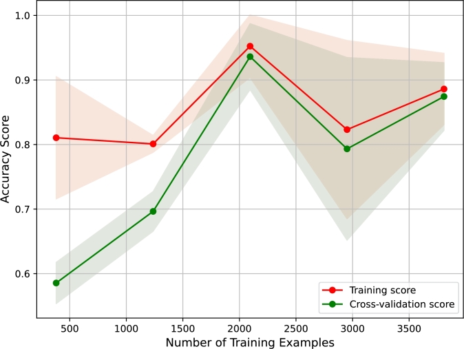
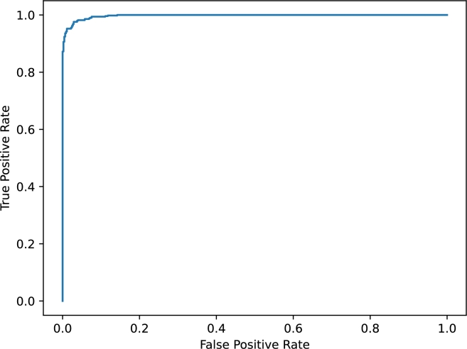
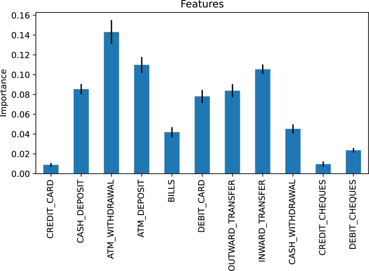
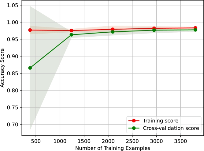
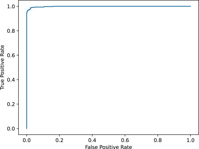
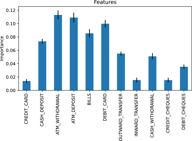
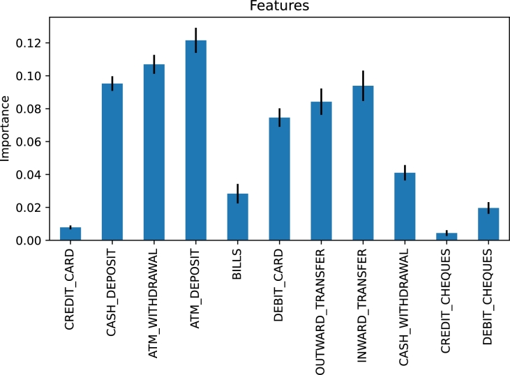
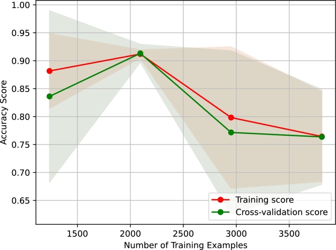
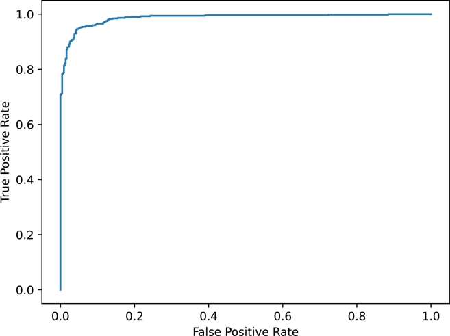
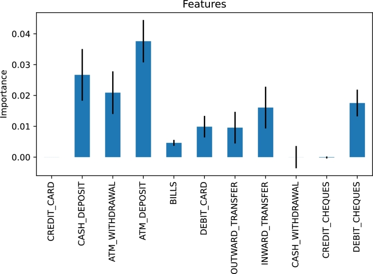
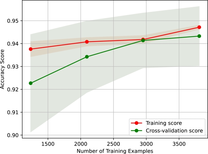
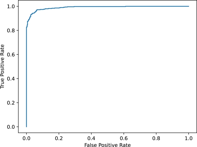
The best-achieved accuracy of our neural network is 0.944. Considering the positive class as the special customer group, the best-achieved precision score is 0.948, the best-achieved recall score is 0.951, the best-achieved F score is 0.95, and the best-achieved ROC–AUC score is 0.98. Fig. 2 shows the learning curve of our neural network, plotting the accuracy score against the number of training examples. Fig. 2 suggests an apparent variation in the performance of our neural network. Fig. 3 shows the ROC curve of our neural network. Lastly, Fig. 4 presents the feature importance chart of our neural network model.

Figure 2.

Learning curve of our neural network for unnormalized data.

Figure 3.

ROC curve of our neural network for unnormalized data.

Figure 4.

Feature importance chart of our neural network for unnormalized data.

Neural networks: the case of normalized data $D_2$

We implemented MLPClassifier from sklearn.neural_network. We set the parameter hidden_layer_sizes=(200,200), where the $i^{th}$ element represents the number of neurons in the $i^{th}$ hidden layer. The rest of the parameters of MLPClassifier were left to the default values [49].

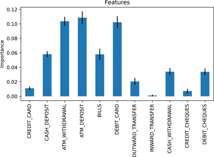
The best-achieved accuracy score of our neural network is 0.978. Considering the positive class as the special customer group, the best-achieved precision score is 0.986, the best-achieved recall score is 0.971, the best-achieved F score is 0.978, and the best-achieved ROC–AUC score is 0.998. Fig. 5 shows the learning curve of our neural network concerning the accuracy score against the number of training examples. Fig. 6 shows the ROC curve of our neural network, which is not surprising given the best-achieved scores of our model. Lastly, Fig. 7 presents the feature importance chart of our neural network model.

Figure 5.

Learning curve of our neural network for normalized data.

Figure 6.

ROC curve of our neural network for normalized data.

Figure 7.

Feature importance chart of our neural network for normalized data.

Decision Trees: the case of unnormalized data $D_1$

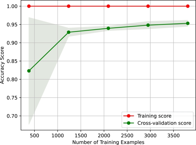
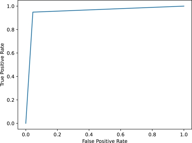
We utilized DecisionTreeClassifier from sklearn.tree. We left the parameters of DecisionTreeClassifier to the default values [49]. The best-achieved accuracy score of our decision tree is 0.951. Considering the positive class as the special customer group, the best-achieved precision score is 0.963, the best-achieved recall score is 0.949, the best-achieved F score is 0.956, and the best-achieved ROC–AUC score is 0.952. Fig. 8 shows the learning curve of our decision tree concerning the accuracy score against the number of training examples. Fig. 8 suggests that our decision tree is slightly an overfitting model. Fig. 9 shows the ROC curve of our decision tree, which is consistent with the best-achieved scores of our model. Lastly, Fig. 10 presents the feature importance chart of our decision tree model.

Figure 8.

Learning curve of our decision tree for unnormalized data.

Figure 9.

ROC curve of our decision tree for unnormalized data.

Figure 10.

Feature importance chart of our decision tree for unnormalized data.

Decision Trees: the case of normalized data $D_2$

We utilized DecisionTreeClassifier from sklearn.tree without tampering with the default parameters [49]. The best-achieved accuracy score of our decision tree is 0.954. Considering the positive class as the special customer group, the best-achieved precision score is 0.965, the best-achieved recall score is 0.951, the best-achieved F score is 0.958, and the best-achieved ROC–AUC score is 0.954. Fig. 11 shows the learning curve of our decision tree, plotting the accuracy score against the number of training examples. Fig. 11 suggests that our decision tree is slightly an overfitting model. Fig. 12 shows the ROC curve of our decision tree. Lastly, Fig. 13 presents the feature importance chart of our decision tree model.

Figure 11.

Learning curve of our decision tree for normalized data.

Figure 12.

ROC curve of our decision tree for normalized data.

Figure 13.

Feature importance chart of our decision tree for normalized data.

Support Vector Machines: the case of unnormalized data $D_1$

We employed svm.SVC() from sklearn. We left the parameters of svm.SVC() to the default values [49] except the parameter “probability” was set to “True” to generate the probabilities of the predictions made by the classifier to be able to compute the ROC–AUC score based on the probabilities of the predictions rather than the predictions themselves.

The best-achieved accuracy score of our support vector machine is 0.694. Considering the positive class as the special customer group, the best-achieved precision score is 1.0, the best-achieved recall score is 0.448, the best-achieved F score is 0.618, and the best-achieved ROC–AUC score is 0.987. Fig. 14 shows the learning curve of our support vector machine concerning the accuracy score against the number of training examples. Fig. 14 reveals a variation in the performance of our support vector machine. Fig. 15 shows the ROC curve of our support vector machine, which is in accord with the best-achieved scores of our model. Lastly, Fig. 16 presents the feature importance chart of our support vector machine model.

Figure 14.

Learning curve of our support vector machine for unnormalized data.

Figure 15.

ROC curve of our support vector machine for unnormalized data.

Figure 16.

Feature importance chart of our support vector machine for unnormalized data.

Support Vector Machines: the case of normalized data $D_2$

We employed svm.SVC() from sklearn without altering the default parameters [49] except the parameter “probability” was set to “True” to generate the probabilities of the predictions made by the classifier to be able to compute the ROC–AUC score using the probabilities of the predictions rather than the predictions themselves.

The best-achieved accuracy score of our support vector machine is 0.940. Considering the positive class as the special customer group, the best-achieved precision score is 0.978, the best-achieved recall score is 0.904, the best-achieved F score is 0.939, and the best-achieved ROC–AUC score is 0.990. Fig. 17 shows the learning curve of our support vector machine concerning the accuracy score against the number of training examples. Fig. 18 shows the ROC curve of our support vector machine, which aligns with our model's best-achieved scores. Lastly, Fig. 19 presents the feature importance chart of our support vector machine model.

Figure 17.

Learning curve of our support vector machine for normalized data.

Figure 18.

ROC curve of our support vector machine for normalized data.

Figure 19.

Feature importance chart of our support vector machine for normalized data.

4.3. Discussion

Recall that our objective of this study is to test the hypothesis that highly-valued bank customers with current accounts can be identified by the frequency and amount of their transactions with the bank. To this end, in our experiments reported earlier, we segmented 4760 real customers based on transactional behavior in a local bank in Jordan. Thus, we partitioned our customer data (representing transactions between 1 June 2021 and 30 June 2022) into two groups. The two constructed clusters are called special and standard. We found that the special cluster includes customers with frequent transactions in relatively large amounts of money. In contrast, the standard cluster includes customers with few transactions in relatively small amounts of money. Customers who make more transactions in large amounts of money probably have more value to the bank. This is realistic because our data includes customers with current accounts. One may say that the balance of a customer account can be sufficient to estimate the value of the customer to the bank. This can be true for other bank accounts, such as savings or investment accounts. But the balance might not be indicative for current accounts where money flows in and out quite frequently. Our results in the previous section confirm our hypothesis that customers with a high frequency of transactions in large amounts are grouped in one cluster, as verified by the three clustering algorithms employed for segmenting our customers.

In the second stage of our experiments, using the segmented data, we constructed three classification models to be exploited for classifying bank customer accounts as special or standard. One may question the purpose of creating predictive models given that we can use clustering to predict if a customer must be with a special account. Although we can use clustering to accomplish this task, having a classification model to label customers as special or standard is more efficient and convenient. Consider the case where clustering is applied; such a process needs a professional user and is time-consuming. Note that a classification model is constructed once (or from time to time) and used many times with less effort and time. Now, we comment on the performance of our classification models. Our neural network model outperforms the other models with an accuracy of 97.8%, whereas the decision tree and support vector machine have comparable accuracy of 95.4% and 94%, respectively. Our results on the constructed classification models suggest that neural networks and support vector machines are sensitive to whether the data is normalized. In contrast, decision trees perform, in our experiments, similarly for normalized and unnormalized data. In the case of unnormalized data, our neural network needed to be larger with more neurons and a third layer to exhibit high performance close to the case of normalized data. Our support vector machine does not perform well in the case of unnormalized data, and we could not find a way to improve its accuracy. Moreover, as suggested by the feature importance charts presented earlier, transaction types have widely different effects in predicting the class of customers (i.e., special or standard). Although the three models agree to a certain degree that ATM withdrawal and ATM deposit transactions are the most important predictors, they differ in the second most important indicator. Our neural network and support vector machine suggest that debit card transactions are the second most crucial predictor. Conversely, the decision tree model states that cash deposit transactions are the second most important predictor.

Once a bank identifies a customer as special, the bank may treat the customer differently to please the customer and encourage the customer to keep the account active with more financial transactions. For instance, the bank may offer special customers high cashback rates on some credit card transactions or reduce fees on some transactions, such as money transfers. The bank may also provide special customers with some facilities usually unavailable for standard customers. Additionally, identifying customers is streamlined further by employing our classification models such that we effectively recognize customers eligible for special treatment and offers. If, on the opposite, a bank decides to classify their customer accounts manually or using clustering exclusively, then the bank needs massive, costly staffing.

To summarize the impact of our findings on the banking sector, we stress two dimensions. For the first dimension, our results are encouraging banks to identify highly valued bank customers based on their transactions because that will help banks set effective marketing plans associated closely with the most-used channels of transactions by the highly-valued customers; hence, in turn, successful marketing (with customized offers) will enhance banks' retention tactics of the most valued customers for the long run. For the second dimension of the impact of our results, we note that recognizing highly-valued customers based on their transactions will allow banks to focus more on the preferences of those most profitable to the banks; thus, in light of these preferences, banks can fine-tune their services or launch new ones towards enhancing the banking experience of the most valued customers to the bank.

4.4. Our study's limitation

Even though the data of this study is geographically restricted in Jordan, the study's conclusion is likely applicable universally since banks use comparable data worldwide, especially concerning transactional data, which is the focus of this study. Nonetheless, the limitation of this study is that our data set covers only the customers of one bank. That is, if other, more diverse data (drawn from more than one bank) is available, then our experiments can be replicated, and hence results might be strengthened further.

Another limitation of our study is that our models rely substantially on customers' historical transactional data availability. Thus, our predictive models presented in this article help recognize highly-valued customers with a history of bank transactions. Therefore, banks may have to adopt another strategy for identifying potentially high-value customers (with no historical transactions with the bank) who are newly signing in with the bank.

As our study's purposes require focusing on transactional data for bank customer valuation, our results do not imply that banks must rely only on transactional data to understand their customers. Our results must be taken carefully because transactional data alone might not give insights into why customers behave with the bank in specific ways. It might be the case that some bank customers could be more profitable to a bank if their perception of the bank services changes or the bank triggers them to be so. Thus, banks must always combine different kinds of data (demographic, digital behavior, customer's banking lifetime, etc.) and exercise varying analyses, such as customers' responses to surveys and customer churn analysis, to get a holistic picture of their customer behavior.

5. Conclusion and future perspective

We addressed the problem of identifying highly-valued (i.e., special) customers with current bank accounts according to their transactions with the bank. To verify the hypothesis that highly-valued bank customers can be recognized by the frequency and amount of their transactions with the bank, we processed a sample of 407851 genuine transactions of randomly selected customers in a local bank in Jordan. We clustered our customers into two groups: special and standard. The special cluster includes customers with frequent transactions involving large amounts of money compared to the standard group that subsumes customers with somewhat fewer transactions involving small amounts of money. Thus, our clustering experiments confirmed the hypothesis that highly-valued bank customers can be recognized by the frequency and amount of their transactions with the bank. Then, we built classification models that facilitate the process of customer categorization into special and standard accounts. By customer classification as special or standard, banks can better understand their customer's needs and hence be more productive in customized, targeted marketing plans and more effective concerning customer retention strategies.

Moreover, since our findings imply that ATM withdrawals and ATM deposits are likely the most critical indicators for identifying highly-valued bank customers, banks may invest considerably in strengthening these transaction channels. We recommend that banks boost their ATM network by ensuring that ATMs are abundant in plenty, carefully placed in diverse locations, easy to access, with a friendly interface, and designed for ergonomics. Further, banks may introduce additional facilities and services that can be transacted through ATMs, and banks can associate offers and rewards with ATM transactions for those identified as special customers.

In the future, we aim to collect further practical evidence on understanding customer behavior in banking services related to loans and investment strategies. Likewise, future research may investigate other types of bank customers and examine what characteristics are crucial to effectively recognizing such latent kinds of customers. Additionally, to enhance the search for efficient predictive models in analyses of transactional bank data, one may explore the impact of employing metaheuristic search algorithms; see recent advances in this line of research, e.g., [28], [23], [22], [1], [2].

CRediT authorship contribution statement

Samer Nofal: Writing – review & editing, Writing – original draft, Visualization, Validation, Supervision, Software, Resources, Project administration, Methodology, Investigation, Formal analysis, Data curation, Conceptualization.

Declaration of Competing Interest

The authors declare that they have no known competing financial interests or personal relationships that could have appeared to influence the work reported in this paper.

Data availability statement

The author does not have permission to share data.

References

- 1.Agushaka Jeffrey O., Ezugwu Absalom E., Abualigah Laith. Dwarf mongoose optimization algorithm. Comput. Methods Appl. Mech. Eng. 2022;391 [Google Scholar]
- 2.Agushaka Jeffrey O., Ezugwu Absalom E., Abualigah Laith. Gazelle optimization algorithm: a novel nature-inspired metaheuristic optimizer. Neural Comput. Appl. 2023;35(5):4099–4131. [Google Scholar]
- 3.Ahmad Saleem, Salem Sultan, Khan Yousaf Ali, Ashraf I.M. A machine learning-based biding price optimization algorithm approach. Heliyon. 2023;9(10) doi: 10.1016/j.heliyon.2023.e20583. [DOI] [PMC free article] [PubMed] [Google Scholar]
- 4.Alghamdi Abdullah. A hybrid method for customer segmentation in Saudi Arabia restaurants using clustering, neural networks and optimization learning techniques. Arab. J. Sci. Eng. 2023;48(2):2021–2039. doi: 10.1007/s13369-022-07091-y. [DOI] [PMC free article] [PubMed] [Google Scholar]
- 5.Ankerst Mihael, Breunig Markus M., Kriegel Hans-Peter, Sander Jörg. Optics ordering points to identify the clustering structure. SIGMOD Rec. jun 1999;28(2):49–60. [Google Scholar]
- 6.Apicella Andrea, Donnarumma Francesco, Isgrò Francesco, Prevete Roberto. A survey on modern trainable activation functions. Neural Netw. 2021;138:14–32. doi: 10.1016/j.neunet.2021.01.026. [DOI] [PubMed] [Google Scholar]
- 7.Alireza Athari Seyed, Irani Farid, Hadood Abobaker AlAl. Country risk factors and banking sector stability: do countries' income and risk-level matter? Evidence from global study. Heliyon. 2023;9(10) doi: 10.1016/j.heliyon.2023.e20398. [DOI] [PMC free article] [PubMed] [Google Scholar]
- 8.bankaudigroup.com . 2021. https://www.bankaudigroup.com/group/publications Bank audi economic research - Jordan report. [Google Scholar]
- 9.Bartels Catja. 2022 3rd. 2022. Cluster analysis for customer segmentation with open banking data; pp. 87–94. (Asia Service Sciences and Software Engineering Conference). [Google Scholar]
- 10.Ben Ncir Chiheb-Eddine, Ben Mzoughia Mohamed, Qaffas Alaa, Bouaguel Waad. Evolutionary multi-objective customer segmentation approach based on descriptive and predictive behaviour of customers: application to the banking sector. J. Exp. Theor. Artif. Intell. 2022:1–23. [Google Scholar]
- 11.Bezbochina Alexandra, Stavinova Elizaveta, Kovantsev Anton, Chunaev Petr. International Conference on Computational Science. Springer; 2022. Dynamic classification of bank clients by the predictability of their transactional behavior; pp. 502–515. [Google Scholar]
- 12.Boser Bernhard E., Guyon Isabelle M., Vapnik Vladimir N. Proceedings of the Fifth Annual Workshop on Computational Learning Theory, COLT '92. Association for Computing Machinery; 1992. A training algorithm for optimal margin classifiers; pp. 144–152. [Google Scholar]
- 13.Boudet Julien, Gregg Brian, Rathje Kathryn, Stein Eli, Vollhardt Kai. McKinsey & Company: Marketing & Sales. 2019. The future of personalization—and how to get ready for it. [Google Scholar]
- 14.Breiman Leo. Random forests. Mach. Learn. 2001;45:5–32. [Google Scholar]
- 15.Breiman Leo, Friedman J.H., Olshen R.A., Stone C.J. Wadsworth; 1984. Classification and Regression Trees. [Google Scholar]
- 16.Cortes Corinna, Vapnik Vladimir. Support-vector networks. Mach. Learn. 1995;20(3):273–297. [Google Scholar]
- 17.Costa Vinícius G., Pedreira Carlos E. Recent advances in decision trees: an updated survey. Artif. Intell. Rev. 2022:1–36. [Google Scholar]
- 18.Kumar Dash Manoj, Kumar Sahu Manash, Bhattacharyya Jishnu, Sakshi Shivam. Customer-Centricity in Organized Retailing: A Guide to the Basis of Winning Strategies. Springer; 2023. Customer segmentation: smpi model; pp. 39–90. [Google Scholar]
- 19.Dogan Onur, Seymen Omer Faruk, Hiziroglu Abdulkadir. Customer behavior analysis by intuitionistic fuzzy segmentation: comparison of two major cities in Turkey. Int. J. Inf. Technol. Decis. Mak. 2022;21(02):707–727. [Google Scholar]
- 20.Durojaye D.I., Obunadike Georgina. Analysis and visualization of market segementation in banking sector using kmeans machine learning algorithm. FUDMA J. Sci. 2022;6(1):387–393. [Google Scholar]
- 21.Ester Martin, Kriegel Hans-Peter, Sander Jörg, Xu Xiaowei, et al. Kdd. vol. 96. 1996. A density-based algorithm for discovering clusters in large spatial databases with noise; pp. 226–231. [Google Scholar]
- 22.Ezugwu Absalom E., Agushaka Jeffrey O., Abualigah Laith, Mirjalili Seyedali, Gandomi Amir H. Prairie dog optimization algorithm. Neural Comput. Appl. 2022;34(22):20017–20065. doi: 10.1007/s00521-022-07705-4. [DOI] [PMC free article] [PubMed] [Google Scholar]
- 23.Ghasemi Mojtaba, Zare Mohsen, Zahedi Amir, Akbari Mohammad-Amin, Mirjalili Seyedali, Abualigah Laith. Geyser inspired algorithm: a new geological-inspired meta-heuristic for real-parameter and constrained engineering optimization. J. Bionics Eng. 2023:1–35. [Google Scholar]
- 24.Griva Anastasia, Zampou Eleni, Stavrou Vasilis, Papakiriakopoulos Dimitris, Doukidis George. A two-stage business analytics approach to perform behavioural and geographic customer segmentation using e-commerce delivery data. J. Decis. Syst. 2023:1–29. [Google Scholar]
- 25.Hadad Yossi, Keren Baruch. A decision-making support system module for customer segmentation and ranking. Expert Syst. 2023;40(2) [Google Scholar]
- 26.Heidari Safanaz, Radfar Reza, Alborzi Mahmood, Kazemi Mohammad Ali Afshar, Ghatari Ali Rajabzadeh. Clustering algorithm for electronic services customers: a case study of the banking industry. Int. J. Nonlinear Anal. Appl. 2022 [Google Scholar]
- 27.Hosseini Maryam, Abdolvand Neda, Harandi Saeedeh Rajaee. Two-dimensional analysis of customer behavior in traditional and electronic banking. Digit. Bus. 2022;2(2) [Google Scholar]
- 28.Hu Gang, Guo Yuxuan, Wei Guo, Abualigah Laith. Genghis Khan shark optimizer: a novel nature-inspired algorithm for engineering optimization. Adv. Eng. Inform. 2023;58 [Google Scholar]
- 29.Incorporation Gartner. The state of marketing budget and strategy. 2022. https://www.gartner.com/en/marketing/research/annual-cmo-spend-survey-research
- 30.Amar Johri, Wasiq Mohammad, Kaur Harpreet, Asif Mohammad. Assessment of users' adoption behaviour for stock market investment through online applications. Heliyon. 2023;9(9) doi: 10.1016/j.heliyon.2023.e19524. [DOI] [PMC free article] [PubMed] [Google Scholar]
- 31.Joung Junegak, Kim Harrison. Interpretable machine learning-based approach for customer segmentation for new product development from online product reviews. Int. J. Inf. Manag. 2023;70 [Google Scholar]
- 32.Junarsin Eddy, Pelawi Rizky Yusviento, Kristanto Jordan, Marcelin Isaac, Pelawi Jeffrey Bastanta. Does fintech lending expansion disturb financial system stability? Evidence from Indonesia. Heliyon. 2023;9(9) doi: 10.1016/j.heliyon.2023.e18384. [DOI] [PMC free article] [PubMed] [Google Scholar]
- 33.Kanchanapoom Kessara, Chongwatpol Jongsawas. Integrated customer lifetime value (clv) and customer migration model to improve customer segmentation. J. Market. Anal. 2023;11(2):172–185. [Google Scholar]
- 34.Kasri Rahmatina Awaliah, Surya Indrastomo Banjaran, Dhani Hendranastiti Nur, Budi Prasetyo Muhammad. Digital payment and banking stability in emerging economy with dual banking system. Heliyon. 2022;8(11) doi: 10.1016/j.heliyon.2022.e11198. [DOI] [PMC free article] [PubMed] [Google Scholar]
- 35.Komatsu Hidenori, Kimura Osamu. Customer segmentation based on smart meter data analytics: behavioral similarities with manual categorization for building types. Energy Build. 2023;283 [Google Scholar]
- 36.Kumar Parul, Islam Md Aminul, Pillai Rekha, Sharif Taimur. Analysing the behavioural, psychological, and demographic determinants of financial decision making of household investors. Heliyon. 2023;9(2) doi: 10.1016/j.heliyon.2023.e13085. [DOI] [PMC free article] [PubMed] [Google Scholar]
- 37.Li Chunling, Khaliq Nosherwan, Chinove Leslie, Khaliq Usama, Ullah Mirzat, Lakner Zoltán, Popp József. Perceived transaction cost and its antecedents associated with fintech users' intention: evidence from Pakistan. Heliyon. 2023;9(4) doi: 10.1016/j.heliyon.2023.e15140. [DOI] [PMC free article] [PubMed] [Google Scholar]
- 38.Li Jia, Sun Zhoutianyang. Application of deep learning in recognition of accrued earnings management. Heliyon. 2023;9(3) doi: 10.1016/j.heliyon.2023.e13664. [DOI] [PMC free article] [PubMed] [Google Scholar]
- 39.Li Jiaqi, Wang Xiaoyan, Ahmad Saleem, Huang Xiaobing, Khan Yousaf Ali. Optimization of investment strategies through machine learning. Heliyon. 2023;9(5) doi: 10.1016/j.heliyon.2023.e16155. [DOI] [PMC free article] [PubMed] [Google Scholar]
- 40.Li Yue, Qi Jianfang, Chu Xiaoquan, Mu Weisong. Customer segmentation using k-means clustering and the hybrid particle swarm optimization algorithm. Comput. J. 2023;66(4):941–962. [Google Scholar]
- 41.Meng Fanlin, Ma Qian, Liu Zixu, Zeng Xiao-Jun. Multiple dynamic pricing for demand response with adaptive clustering-based customer segmentation in smart grids. Appl. Energy. 2023;333 [Google Scholar]
- 42.Minsky Marvin, Papert Seymour. MIT Press; Cambridge, MA: 1969. Perceptrons, vol. 6; pp. 318–362. [Google Scholar]
- 43.Mosa Mona, Agami Nedaa, Elkhayat Ghada, Kholief Mohamed. A novel hybrid segmentation approach for decision support: a case study in banking. Comput. J. 2022 [Google Scholar]
- 44.Nguyen Huan Huu, Ngo Vu Minh, Phuong Le Thao Thi, Nguyen Phuc Van. Do investors' personalities predict market winners? Experimental setting and machine learning analysis. Heliyon. 2023;9(4) doi: 10.1016/j.heliyon.2023.e15273. [DOI] [PMC free article] [PubMed] [Google Scholar]
- 45.Qureshi Moiz, Ahmad Nawaz, Ullah Saif, Raza ul Mustafa Ahmed. Forecasting real exchange rate (reer) using artificial intelligence and time series models. Heliyon. 2023;9(5) doi: 10.1016/j.heliyon.2023.e16335. [DOI] [PMC free article] [PubMed] [Google Scholar]
- 46.Rajput Lucky, Singh Shailendra Narayan. 2023 13th International Conference on Cloud Computing, Data Science & Engineering (Confluence) IEEE; 2023. Customer segmentation of e-commerce data using k-means clustering algorithm; pp. 658–664. [Google Scholar]
- 47.Rumelhart David E., Hinton Geoffrey E., Williams Ronald J. Learning representations by back-propagating errors. Nature. 1986;323(6088):533–536. [Google Scholar]
- 48.Schmidhuber Jürgen. Deep learning in neural networks: an overview. Neural Netw. 2015;61:85–117. doi: 10.1016/j.neunet.2014.09.003. [DOI] [PubMed] [Google Scholar]
- 49.scikit-learn.org, Machine learning library, accessed: 2023/01/03.
- 50.Shi Jianbo, Malik Jitendra. Normalized cuts and image segmentation. IEEE Trans. Pattern Anal. Mach. Intell. 2000;22(8):888–905. [Google Scholar]
- 51.Sivaguru M. Dynamic customer segmentation: a case study using the modified dynamic fuzzy c-means clustering algorithm. Granul. Comput. 2023;8(2):345–360. [Google Scholar]
- 52.TheGlobalEconomy.com Bank assets to gdp country rankings 2020. https://www.theglobaleconomy.com/rankings/bank_assets_GDP/
- 53.Nur Uddin Mohammad, Ur Rashid Md Harun, Rahman Md Tahidur. Profitability, marketability, and csr disclosure efficiency of the banking industry in Bangladesh. Heliyon. 2022;8(11) doi: 10.1016/j.heliyon.2022.e11904. [DOI] [PMC free article] [PubMed] [Google Scholar]
- 54.von Luxburg Ulrike. A tutorial on spectral clustering. Stat. Comput. 2007;17(4):395–416. [Google Scholar]
- 55.R. Yudaruddin, W. Soedarmono, B.A. Nugroho, Z. Fitrian, M. Mardiany, A.H. Purnomo, E.N. Santi, Financial technology and bank stability in an emerging market economy, 2023. [DOI] [PMC free article] [PubMed]
Associated Data
This section collects any data citations, data availability statements, or supplementary materials included in this article.