Abstract
Wildfire is an important natural disturbance agent in Canadian forests, but it has also caused significant economic damage nationwide. Spatial fire growth models have emerged as important tools for representing wildfire dynamics across diverse landscapes, enabling the mapping of key wildfire hazard metrics such as location-specific burn probabilities or likelihoods of fire ignition. While these summary metrics have gained popularity, they often fall short in capturing the directional spread of wildfires and their potential spread distances. The metrics depicting the directional spread of wildfire can be derived from raw outputs generated with fire growth models, such as the perimeters and ignition locations of individual fires, but extracting this information requires complex data processing. To address this data gap, we present PostBP, an open-source Python package designed for post-processing the raw outputs of fire growth models — the ignition locations and perimeters of individual fires simulated over multiple stochastic iterations — into a matrix of fire spread likelihoods between all pairs of forest patches in a landscape. The PostBP also generates several other summary outputs, such as the source-sink ratio and the fire spread rose diagram. We provide an overview of PostBP's capabilities and demonstrate its practical application to a forested landscape.
-
•
Wildfire growth models generate large amounts of outputs, which are hard to summarize for practical decision-making.
-
•
The PostBP package calculates the summary metrics characterizing the directional spread of wildfires.
-
•
The fire risk summaries generated with PostBP can support the assessments of wildfire risk and mitigation measures.
Keywords: Fire growth modeling, Wildfires, Fire ignition, Fire perimeter, Fire spread likelihood, Source-sink ratio, Burn-P3
Method name: PostBP: Post-processing the outputs of Fire Growth Models
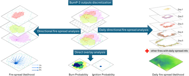
Graphical abstract
Specifications table
| Subject area: | Earth and Planetary Sciences |
| More specific subject area: | Wildfire, fire growth modeling, wildfire risk mapping |
| Name of your method: | PostBP: Post-processing the outputs of Fire Growth Models |
| Name and reference of original method: | N.A. |
| Resource availability: | GitHub repository: https://github.com/nliu-cfs/postbp Documentation: https://nliu-cfs.github.io/postbp/ |
Background
Wildfire, while being a natural process in Canadian forests [1], pose significant threats to human communities in forested regions [[2], [3], [4]]. Land managers invest substantial resources into the assessment of wildfire regimes and employ various modeling tools to predict the risks of wildfires in forest landscapes [[5], [6], [7]]. Many assessments use spatial fire growth models (FGMs) to evaluate the outcomes of fire ignition events. An extension of FGMs, known as burn probability models, simulates numerous stochastic ignitions and the spread of fires from the ignition locations; these tools have become popular for predicting forest fire behavior at the landscape scale [5,6,[8], [9], [10], [11], [12]]. Burn probability models generate the perimeters of individual fires using probabilistic estimates of ignitions, fuel conditions, topographic features, and weather conditions. The outputs of burn probability models help evaluate wildfire risk mitigation measures, such as preventive fuel treatments [11,13] and assist the strategic planning of suppression efforts [12,14]. Examples of popular burn probability models include the Canadian Burn-P3 model [5], the FSim model in the USA [6] and the Australian Phoenix model [7].
The primary output of burn probability models is a set of ignition locations and perimeters of individual fires, simulated stochastically over multiple iterations, with each iteration representing a single burn year. Predicted fire perimeters depict the likely spread of wildfires across the landscape of interest. The outputs with multiple wildfire perimeters are stored in multiple overlapping geographic polygons (or spatial data layers), which makes it cumbersome to use in practical decision-making. A common remedy is to condense raw fire model outputs into summary maps showing, for each location, the likelihoods of wildfire occurrence or other fire behavior characteristics, such as fire intensity or fuel consumption [15]. However, these simplified summaries do not communicate information about the directional spread of fires and their likely spread distances.
In applications involving neighbourhood analyses, the perimeters of wildfires spreading to a given site from elsewhere can be summarized using the fireshed concept [16]. For a forest patch i, the fireshed delineates the area from which a fire could potentially ignite and spread to i. An opposite concept to a fireshed is a fireplain that delineates the area that could be affected by fires originating from a given location [17]. Another useful summary metric is the source-sink ratio [18] that defines the ratio between the expected number of fires originating from a given location and the expected number of fires spreading to that location from elsewhere. A more complex approach is to map the fire spread vectors and likelihoods between all pairs of locations across the landscape [13,19], which enables characterizing the directional spread of wildfires. For a given pair of forest patches i,j, this approach defines the likelihood that a fire ignited in i will spread to j. The landscape is characterized by a set of fire spread vectors between all pairs of locations; this set preserves information about prevailing fire spread directions and distances and thus helps better facilitate effective planning of wildfire risk mitigation and suppression activities [13,19]. The novelty of our approach is that it enables a detailed mapping of fire spread pathways, and the depiction of likely directions and fire spread distances, which provides important insights for managing wildfire risks and designing fire mitigation measures.
Method details
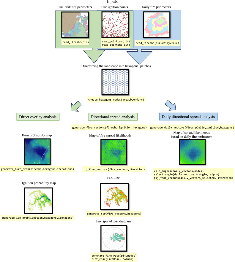
Deriving fire spread likelihoods from raw burn probability model outputs, while numerically straightforward, involves several complex data processing steps. We present PostBP, an open-source Python library for post-processing raw FGM outputs and calculating a suite of summary fire hazard metrics. PostBP offers three post-processing options for analyzing FGM outputs (Fig. 1). Option 1 (“Direct overlay analysis”) generates maps of mean burn and ignition likelihoods for a user-defined set of forest landscape patches. Option 2 (“Directional fire spread analysis”) uses the ignition locations and final perimeters of individual fires to generate vectors of spread likelihoods between all pairs of forest patches in a landscape, along with a map of source-sink ratios and a fire spread rose diagram. Option 3 (“Daily directional fire spread analysis”) is similar to option 2 but generates fire spread likelihoods and summary outputs from sequences of daily fire perimeters instead of the final fire perimeters utilized in option 2.
Fig. 1.
A summary of PostBP functions.
Method description
We developed the library to work with the standard outputs of the Canadian Burn-P3 fire growth simulation model [5,8]. Note that the library can process outputs from other FGMs if their format aligns with the Burn-P3 outputs. The standard output of Burn-P3 simulations typically includes an ESRI shapefile with the perimeters of simulated fires (stored as polygons) and key parameters characterizing individual fires. The attribute table in this shapefile stores information such as the model iteration number (in the ‘iteration’ column) and the simulated fire identifier (in the ‘fire’ column). Another important output from Burn-P3 is the X-Y coordinate location of the ignition points for each simulated fire [20]. The number of simulated fires within a single model iteration may vary depending on Burn-P3 scenario settings. The most recent Burn-P3+ version [21] that is available from https://burnp3.github.io/BurnP3Plus/ can output the sequences of daily fire perimeters for each simulated fire, with the burn day identifier stored in the ‘day’ column in the attribute table. An older Burn-P3 version that outputs, for each simulated fire, the final perimeters and the ignition locations only is available from https://firegrowthmodel.ca/pages/burnp3_software_e.html.
PostBP offers an option to create an ESRI polygon shapefile with delineated forest patches and calculates all summary fire behavior metrics at the level of individual patches. We conceptualize the landscape as a network, G, consisting of uniformly sized hexagonal patches i. These hexagons can also be interpreted as an interconnected network of nodes, with each node identified by the centroid of a corresponding hexagon. Hexagonal patches are chosen over square shapes because they offer more directions for fire to spread between adjacent patches. To generate the hexagonal patch network, PostBP provides a function called create_hexagons_nodes, which discretizes the landscape into a network of equal-size hexagons of a user-defined size.
Direct overlay analysis
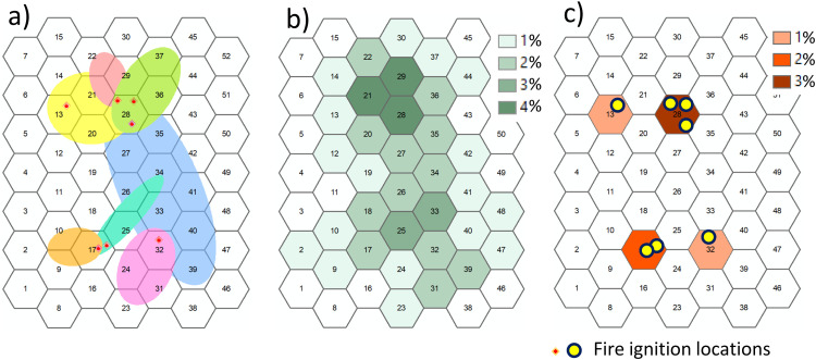
In direct overlay analysis, PostBP uses the ignition locations and perimeters of individual fires simulated with Burn-P3 to calculate summary statistics for each hexagon (patch) i in a landscape by intersecting the fire perimeter data with the network of hexagonal patches (Fig. 2a). Below we describe the two functions used to calculate burn probability and ignition probability values per hexagon.
Fig. 2.
Calculating the ignition probability and burn probability for a set of user-defined hexagons assuming 100 iterations: a) fire perimeters and ignition points; b) burn probability; c) ignition probability. All hexagons overlapping the simulated fire polygons are considered burned areas.
Burn probability
Burn probability (BPi) is calculated as the number of times a fire occurs in hexagon i, bi, divided by the total number of wildfire simulation model iterations, this quotient is multiplied by 100 to express the probability as a percentage (Fig. 2b), i.e.:
| (1) |
The user can apply the function generate_burn_prob and set the minimum threshold for classifying hexagon i as “burned” based on the proportion of its area covered by fire. For example, by setting the argument threshold=0.1*[hexagon area], all hexagons overlapping the simulated fire polygon(s) by 10% or more are treated as burned areas. The default threshold is set to zero, which classifies all hexagons having fires as burned areas, regardless of the degree of spatial overlap.
Ignition probability
PostBP offers a function generate_ign_prob to calculate, for each hexagon i, the ignition probability (IPi) from Burn-P3 outputs. The ignition probability is computed as the number of simulated ignition events in hexagon, gi, divided by the total number of Burn-P3 iterations, N; this quotient is multiplied by 100 to express the probability as a percentage, i.e.:
| (2) |
Fig. 2c shows an example of ignition probability values (IPi) calculated from the simulated ignition locations in each hexagon i in a landscape.
Directional spread analysis
In directional spread analysis, PostBP calculates a matrix of fire spread likelihoods between all pairs of hexagonal patches in a landscape. The primary PostBP functions in this context include: (i) the derivation of fire spread likelihoods, (ii) the computation of source-sink ratios, and (iii) the plotting of a fire spread rose diagram.
Fire spread likelihoods
This function calculates the likelihood, pij, that a fire ignited in hexagon (patch) i will spread to hexagon j in landscape (i.e., hexagonal network) G. The resulting matrix of pij values provides crucial information about the directions and likely spread distances of wildfires and, indirectly, the distribution of linear fire sizes.
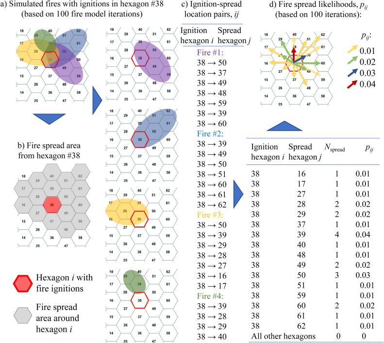
The fire spread likelihood is calculated from the simulated fire perimeters and ignition locations using the algorithm described in Yemshanov et al. [13]. For each pair of forest hexagons i and j, individual fire perimeters from Burn-P3 outputs are used to select the subset of simulated fires ignited in hexagon i and spreading to hexagon j (Fig. 3a). To accomplish this selection, the hexagonal network comprising landscape is overlaid with the fire perimeters. For each fire ignited in hexagon i, all hexagons j to which the fire was able to spread are selected (see shaded area in Fig. 3b). Each selected pair of hexagons (i, j) is represented by a unary vector with the fire origin in i and spread destination in j – was assigned one (Fig. 3c). Note that we counted the fire spread vectors ij without explicitly tracking the possible spread paths from i to j through other patches.
Fig. 3.
Calculating the fire spread likelihoods pij. using on algorithm from [13].
We repeated these calculations for all fire perimeters and the corresponding ignition locations generated by the FGM. For every pair of locations i and j, we have summed the number of times a fire ignited in i was able to spread to j and divided this value by the total number of fire growth model iterations (Fig. 3d).
In the PostBP, the perimeter of each fire is spatially overlapped with the hexagonal network of patches to delineate all hexagons j where a fire ignited in hexagon i was able to spread. For hexagon i that contains the fire ignition point, the generate_fire_vectors function finds all destination hexagons j where fires ignited in i could spread.
Before applying the generate_fire_vectors function, the user should verify whether the shapefile containing the simulated fire perimeters includes one fire per Burn-P3 iteration or a single iteration includes multiple simulated fires. In cases where a single Burn-P3 iteration included more than one fire, an additional function argument, loopby='iteration', must be used. This ensures that the function iterates through both Burn-P3 iterations and the fire IDs within each iteration. Note that the most common Burn-P3 scenarios simulate one fire spread event per iteration [19,22].
The user can set the threshold for the minimum proportion of the burned area in a hexagon that qualifies it as a burned area. For example, by setting the argument threshold=0.1*[hexagon area], all hexagons overlapping the simulated fire polygon(s) by 10% or more are treated as a burned area.
The program assigns unary fire spread vectors for each pair of hexagons (i, j) between the hexagon with the ignition point and every other each hexagon within the simulated fire perimeter. Once the spread vectors ij have been generated for all hexagon pairs and the simulated fires, the pij_from_vectors function computes the fire spread likelihood pij for each hexagon pair (i, j) in landscape G.
Source-sink ratio
The source–sink ratio (SSR) [18] is a metric that assesses the tendency of a landscape patch (i.e., hexagon) to act as either a source or major destination for spreading wildfires. For a hexagon i, PostBP calculates the SSR by examining the number of times i includes the fire ignition point versus the number of times it receives fires spreading from other hexagons j, i.e.:
| (3) |
where pij is the likelihood that a fire ignited in hexagon i spreads to hexagon j and pji is the likelihood that a fire ignited in hexagon j spreads in the opposite direction to hexagon i.
Fire spread rose diagram
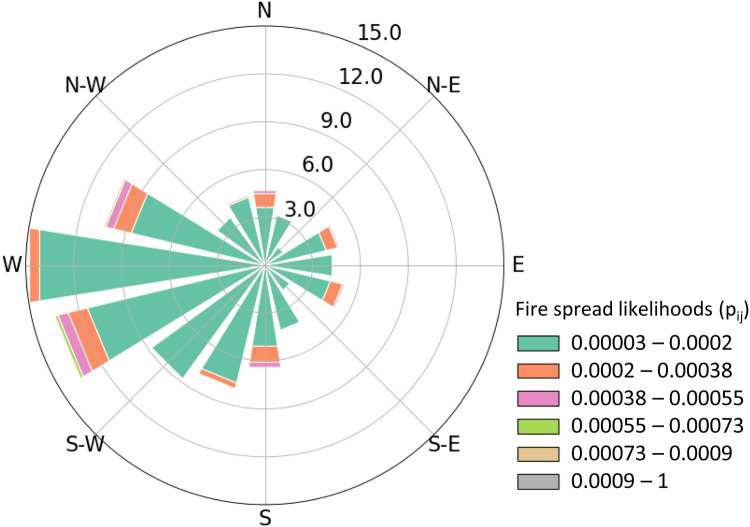
In meteorology, a wind rose diagram depicts the azimuthal distribution of incoming wind directions and speeds at a given location or region. A similar approach can be used to show the distribution of fire spread directions and likelihoods. The fire spread rose diagram shows radial bars representing the directions of incoming fires to a hexagon (patch) of interest i, with the length of each bar indicating the percentage of fires spreading to that hexagon from a particular direction. The bar colours can represent the frequency distribution of the spread likelihoods (or lengths) of fires arriving at i from a particular direction.
In PostBP, the fire spread rose diagram can be generated using either the fire spread likelihood values (pij) or the linear fire spread lengths (len). The function generate_fire_rose prepares the data for plotting, and the function plot_rose creates the diagram. By setting the save argument to True, the fire spread diagram can be saved to a file in the current folder.
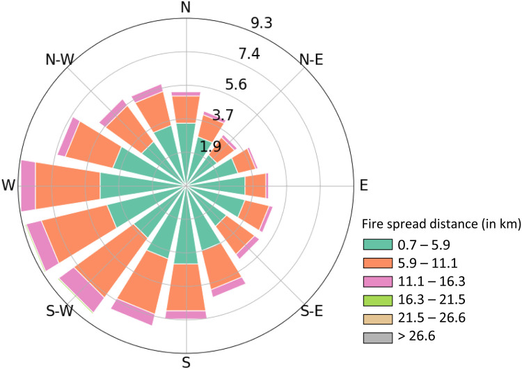
Fig. 4 shows an example of a fire spread rose diagram with color bars depicting the frequencies of fire spread likelihoods (pij) for fires arriving from a particular direction. The diagram shows that most fires arrive from the west (W) and west-southwest (WSW), accounting for 15% and 13.5% of all incoming fires, respectively. Most of the linear spread is contributed by large fires with spread likelihoods below 0.0002.
Fig. 4.
Fire spread rose diagram.
Daily fire spread likelihoods
The most recent Burn-P3+ model version [21] can output the sequences of daily fire perimeters for individual fires and save them as polygons in a single ESRI shapefile. The use of daily fire perimeters enables incorporation of uncertainty regarding the day-to-day fluctuations of local fire spread directions influenced by rapidly changing winds and fire weather conditions. This aspect is particularly useful for assessing the spread risk of large fires that may burn over multiple days. The daily perimeters of individual fires simulated with Burn-P3 are used to generate fire spread vectors (i→j) between consecutive burn days t-1 and t.
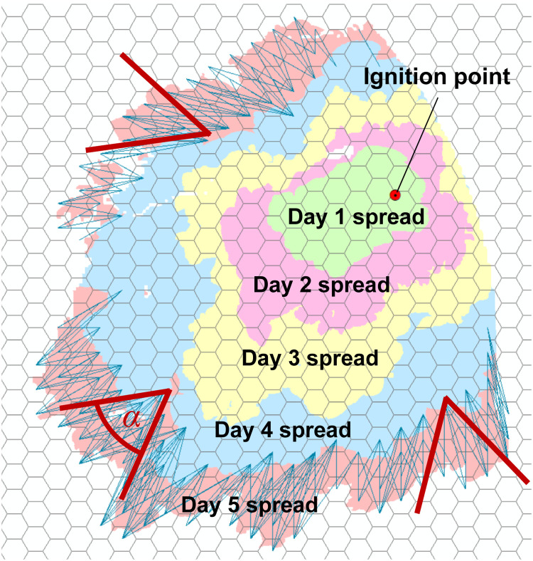
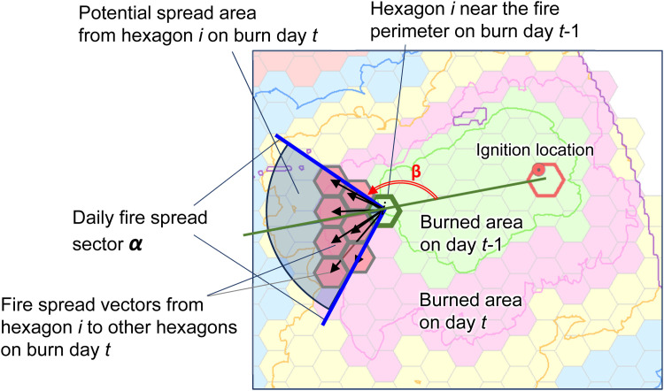
For each burn day t, it is assumed that a fire can only spread from hexagons (patches) i near the perimeter of the fire on the previous burn day t-1 (Fig. 5). It is further assumed that, with respect to every hexagon located near the fire perimeter on burn day t-1, a fire can only spread to other hexagons on the following burn day t if they fall within a defined sector α (see dark red lines in Fig. 5). This sector delineates the plausible range of local spread directions from patch i on burn day t. The size (in degrees) of the sector angle reflects the level of uncertainty about the daily fire spread conditions, with a wider sector implying greater uncertainty. This approach helps account for uncertain variation in local fire spread under rapidly changing daily weather.
Fig. 5.
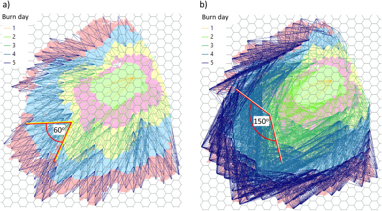
The concept of the daily fire spread sector when calculating the vectors of fire spread on burn day t from hexagons burned on day . The angle, α, of a daily fire spread sector delimits the set of other hexagons j to which fire could spread on day t from patch burned on day . Examples of 60-degree fire spread sectors on burn day 5 extending from hexagons near the fire perimeter on burn day 4 are shown.
To determine the azimuth of the fire spread sector α for a hexagon i, PostBP first calculates the azimuth angle β of the line connecting the fire ignition point to i. Then, it centers sector α around that line as it extends outward from i (Fig. 6). The function select_angle calculates the angle β that is used to position sector α for each hexagon i. For each simulated fire, the daily fire spread vectors between pairs of hexagons (i, j) – shown as black arrows in Fig. 6– are assigned a value of 1, and the calculation of fire spread likelihoods pij between i and j follows the procedure described in Section 2.2.1.
Fig. 6.
Generating the local fire spread sector α and local spread vectors on burn day t from a hexagon i near the perimeter of the fire on burn day t-1.
An application example
We illustrate the functionality of PostBP using outputs from Burn-P3 model simulations for an 80 × 80-km montane forest landscape in Alberta, Canada.
The Burn-P3 outputs required for this example include: (1) a file with the final perimeters of the simulated fires (testDataset_FF.shp with 16,000 stochastic model iterations, one simulated fire per iteration), (2) a file with the sequences of daily perimeters of individual fires for the same number of iterations (testDataset_DFF.shp), and (3) a comma-delimited file with X-Y coordinates of fire ignition points (Dataset_statistics.csv).
Create working environment
PostBP requires the following Python libraries: Math, Pandas, Shapely, Geopandas, Windrose and Matplotlib. All the required libraries are automatically installed when installing the PostBP library. It is recommended to install the PostBP to a working environment other than the base environment. The code snippet in line 1 below installs the PostBP:
# Execute the code while your working environment is activated
1 pip install postbp
Loading Burn-P3 output data
The ESRI shapefiles containing the simulated fire perimeters and ignition points can be loaded using the three following functions. Function read_fireshp loads the files with the final and daily fire perimeters and prepares the data. Function read_pointcsv loads the fire ignition points if this information is provided as a comma-delimited .csv file, and function read_pointshp loads the ignition points if the data is provided as X-Y coordinates in separate columns in the attribute table of the ESRI shapefile with fire perimeters (or in a separate ESRI point shapefile).
To load the daily fire perimeters, one needs to provide the argument daily in read_fireshp function (see the code example in line 6 below). It is also important to check the spatial reference identifiers (SRID) for the loaded data. We recommend using the SRID from the fire perimeter shapefile for all files. Line 2 below imports the library, and lines 3 – 6 load the three Burn-P3 output files:
2 import postbp
3 fireshp = postbp.read_fireshp('testDataset_FF.shp')
4 SRID = fireshp.crs # record spatial reference of fire shapefile
5 ignition = postbp.read_pointcsv('testDataset_Statistics.csv', SRID, x_col='x_coord', y_col='y_coord')
6 fireshpDaily = postbp.read_fireshp('testDataset_DFF.shp', daily=True)
Generate hexagonal patches
Next, we need to create a landscape G of hexagonal patches i. The user needs to delimit the study area boundary and specify a desired hexagon (patch) size. By default, the union of the simulated fire perimeters in the Burn-P3 outputs is used to delimit the area boundary. Alternatively, a user-defined boundary shapefile can be used. The size of a hexagon patch can be defined by setting the hexagon area using the area argument (the default). Alternatively, one can specify the hexagon size by setting its length using the side argument or by its diameter using the diameter argument. Line 7 shows the code snippet to generate the landscape network nodes and 50-ha hexagons. Note that the user can generate hexagons first and then derive the landscape network nodes from hexagons, as shown in lines 8–9:
7 hexagons, nodes = postbp.create_hexagons_nodes(area=500,000, boundaryShp=fireshp)
8 hexagons = postbp.create_hexagons(area=500,000, boundaryShp=fireshp)
9 nodes = postbp.nodes_from_hexagons(hexagons)
Applying the PostBP functions
The code snippet below derives the mean ignition and burn probabilities for 50-ha hexagons (Figs. 7a, 8a) and outputs the data as a GeoDataFrame. The GeoDataFrame format stores the geometry of a landscape patch network in a tabular data structure, which can be exported as Apache GeoParquet, GeoJSON, or ESRI shapefile for visualization, mapping, and quality control.
10 ignProb = postbp.generate_ign_prob(ignition, hexagons, iterations=16,000)
11 burnProb = postbp.generate_burn_prob(fireshp, hexagons, iterations=16,000)
Fig. 7.
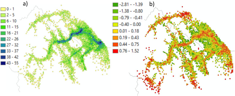
Summary maps: (a) ignition likelihoods; (b) source-sink ratios, SSR. Positive SSR values indicate locations that are predominantly sources of fires that spread to other locations, while negative SSR values show locations that tend to receive fires from elsewhere.
Fig. 8.
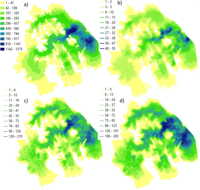
(a) Fire behavior summary maps: a) burn probability; b) fire spread likelihoods, pij, calculated from the final perimeters of individual fires simulated with Burn-P3; c) fire spread likelihoods calculated from the daily fire perimeters, assuming the daily fire spread sector α=60°; d) fire spread likelihoods calculated from the daily fire perimeters, assuming the daily fire spread sector α=150°.
The code in line 12 generates the set of unary fire spread vectors ij between patches i and j for hexagonal network G. Depending on the number and complexity of the simulated fires and computer hardware, this function may take a long time to complete. Besides generating the fire spread likelihoods pij, the variable fire_vectors contains the fire spread vectors ij that are used to calculate the source-to-sink ratio, SSR, and the fire spread rose diagram. The code in line 13 calculates the fire spread likelihoods pij between all pairs of patches (i, j). In the function arguments, the user needs to provide the number of Burn-P3 iterations that will be used to generate the pij values. This number usually corresponds to the total number of iterations in the saved Burn-P3 outputs but could be set to a lower value. The code in line 14 converts and saves the pij values as a GeoDataFrame (Fig. 8b).
12 fire_vectors = postbp.generate_fire_vectors(fireshp, ignition, hexagons)
13 pij = postbp.pij_from_vectors(fire_vectors, iterations=16,000)
14 pij_shp = postbp.pij_to_shp(pij, nodes)
When the shapefile containing the outputs of daily fire perimeters is available, these data can be used to calculate the fire spread likelihoods, pij. In the code snippet in line 15, the function generate_daily_vectors generates the fire spread vectors for each simulated fire from the sequence of daily fire perimeters in the Burn-P3 output files. Notably, this operation is time-consuming. For each simulated fire, the fire_vector_daily variable stores all pairwise spread vectors along with the fire ID, burn day ID, and the ID and location of the ignition point of that fire. Function calc_angles in line 16 uses the locations of the ignition points, the fire spread origin nodes in burn day t-1, and the fire spread destination nodes in burn day t to calculate angle β (i.e., the azimuth angle) for the spread vectors (refer to Fig. 6). The code in lines 17–18 applies the function select_angle to trim the set of fire spread vectors in day t by a user-defined spread sector of size α (e.g., α = 60 or 150° in Fig. 6). Subsequently, lines 19–20 apply the function pij_from_vectors to calculate the fire spread likelihoods pij from the daily fire spread vectors that were calculated from the daily fire perimeters (see line 15) while assuming a chosen spread sector α. Finally, the code in lines 21 - 22 converts the pij values to a GeoDataFrame for visualization, mapping and quality control (see example in Fig. 8c and d).
15 fire_vectors_daily = postbp.generate_daily_vectors(fireshpDaily, ignition, hexagons)
16 fire_vectors_w_angles = postbp.calc_angles(fire_vectors_daily, nodes)
17 daily_vectors_150 = postbp.select_angle(fire_vectors_w_angles, alpha=150)
18 daily_vectors_60 = postbp.select_angle(fire_vectors_w_angles, alpha=60)
19 pij_daily_150 = postbp.pij_from_vectors(daily_vectors_150, iterations=16,000)
20 pij_daily_60 = postbp.pij_from_vectors(daily_vectors_60, iterations=16,000)
21 pij_daily_150_shp = postbp.pij_to_shp(pij_daily_150, nodes)
22 pij_daily_60_shp = postbp.pij_to_shp(pij_daily_60, nodes)
The code in line 23 applies the function generate_ssr to generate the source-sink ratios, SSR. In the function arguments, one needs to specify the name of the variable containing the pairwise fire spread vectors ij (derived in line 12) and the hexagon data. The function generates a GeoDataFrame with the SSR values (Fig. 7b).
23 fireSSR = postbp.generate_ssr(fire_vectors, hexagons)
Plotting the fire spread rose diagram requires the variable containing the calculated fire spread likelihoods, pij. The function generate_fire_rose in line 24 prepares the data frame for plotting. The code calculates the fire spread azimuths for plotting the fire spread rose diagram and the lengths of the fire spread vectors. The user can choose to plot color bars in the diagram based on either fire spread likelihoods pij or fire spread lengths. Line 25 shows the code snippet that plots the fire spread rose diagram using the function plot_rose (Fig. 10). The diagram can be saved in the working folder as a Portable Network Graphic (.png) image file by setting the save argument to True.
24 fireRose = postbp.generate_fire_rose(pij, nodes)
25 postbp.plot_rose(fireRose, column='len', save=False)
Fig. 10.
Fire spread rose diagram.
Examples of PostBP outputs
The fire behavior summary metrics generated by the PostBP library can assist with the planning of fire response and risk mitigation measures in forest landscapes. For example, the map displaying ignition likelihoods helps pinpoint the forest patches that could potentially serve as threatening sources of wildfires (Fig. 7a). The map of the source-sink ratio (SSR) (Fig. 7b) helps distinguish locations that tend to be where fires originate (indicated by positive SSR values) from locations that mostly receive fires from other locations (indicated by negative SSR values).
The burn probability map depicts the likelihoods of fire occurrence in forest patches (hexagons) i (Fig. 8a). Note that PostBP generates all summary metrics at the level of these hexagons, which is a coarser scale than that of the raster burn probability maps produced by Burn-P3. Thus, when generating the hexagonal network G and calculating the summary metrics in PostBP, it is important to consider the minimum burned area threshold that classifies a patch i as a burned area. As mentioned earlier, the default threshold value in PostBP is zero, meaning that any hexagon with a fire present is considered as a burned area regardless of its actual burned proportion.
Fig. 8b shows the map of fire spread likelihoods pij between all pairs of hexagons in landscape G. Because individual ij vectors overlap, the pij values are depicted as a choropleth map, where darker colours indicate higher spread likelihoods and lighter colors indicate lower values. This map helps identify major fire spread corridors and natural barriers.
Figs. 8c, d show maps of daily fire spread likelihoods with spread sectors α=60° and α=150°, respectively. Tracking the daily spread helps account for local variability of fire spread directions, which can be influenced by rapidly changing weather and wind conditions.
The generation of fire spread vectors from the sequences of simulated daily fire perimeters requires specifying the daily fire spread sector α. Fig. 9 illustrates the impact of selecting the sector angle α on the pattern of created fire spread vectors ij, using the example of a single fire that spreads over five days. Fig. 9a shows the fire spread vectors assuming the fire spread sector α=60°, and Fig. 9b shows the spread vectors for α=150°. A wider sector angle implies that fire spread directions may vary within a broader azimuthal sector during a single burn day. The choice of an appropriate sector angle α is driven by assumptions (including the uncertainty in those assumptions) about prevailing wind dynamics, the magnitude of rapid changes in local weather, local topographic conditions, and the history of previous fire disturbances in the area.
Fig. 9.
a) Daily fire spread vectors ij generated within the local spread sector α=60°; b) daily fire spread vectors within the local spread sector α=150°.
A fire spread rose diagram (Fig. 10) depicts the most likely incoming directions of wildfires in the study area. An example diagram in Fig. 10 shows that most fires arrive from the west and southwest. The color bars in the diagram indicate that most incoming fires spread over distances less than 11 km (green and orange bars), with a small fraction of fires capable of spreading more than 11 km (pink bars).
PostBP is a new Python library designed to generate directional data for characterizing wildfire behavior and streamlining the post-processing of fire spread modeling outputs. This tool helps summarize bulky raw outputs of fire growth simulation models into maps of summary metrics and fire spread likelihoods. Such information can be used to support assessments of wildfire risk and assist with the planning of wildfire mitigation and risk reduction measures.
Method validation
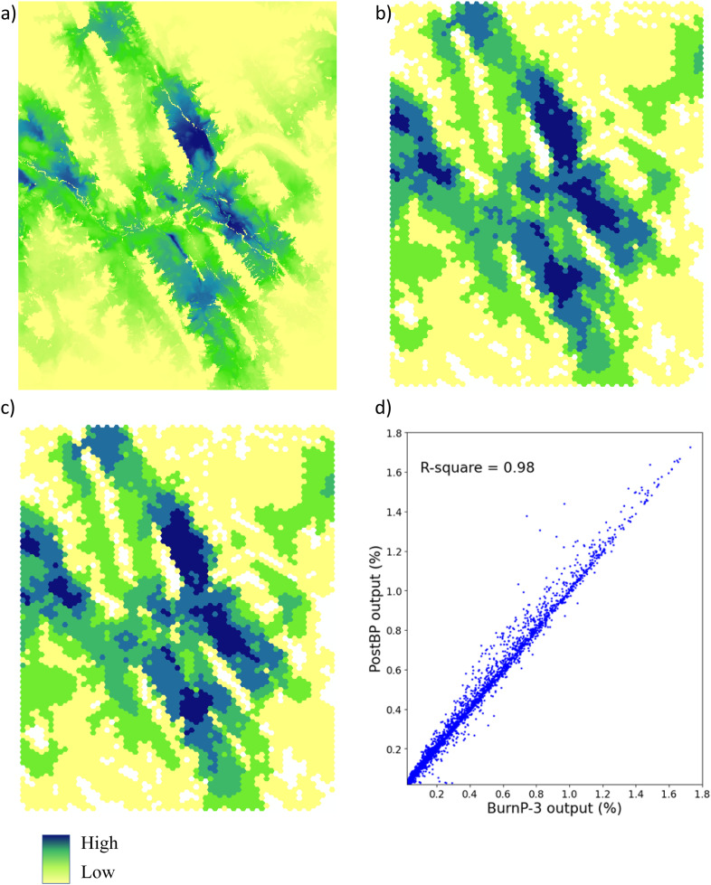
The PostBP library is not designed to model the wildfire spread per se and only creates a suite of summary metrics from the outputs of spatial FGMs to support the assessments of fire risk and mitigation decisions. In this context, the validation was focused on ensuring the algorithm's consistency to handle multiple fire perimeter polygons and verifying the correspondence between the key summary metric generated by the PostBP and the FGM. Since the PostBP calculates the summary outputs at the spatial resolution of user-defined patches (hexagons) we have upscaled the summary maps from the FGM outputs to match the spatial resolution of PostBP’s hexagonal patches. We have compared the burn probability estimates, which is the most common summary metric of wildfire risk [9,11,20,22]. Fig. 11a–c compare the burn probability maps generated by the Burn-P3 fire growth model with the map generated by the PostBP library. The burn probability values in both maps appear close and show high correspondence with R2 = 0.98 (Fig. 11d). Minor discrepancies between the maps can be attributed to the averaging of the burn probability values when upscaling the Burn-P3 outputs to the spatial resolution of hexagonal patches generated by the PostBP library.
Fig. 11.
Comparing the burn probability maps generated by the Burn-P3 model and the PostBP library: a) High-resolution burn probability map generated internally by the Burn-P3 model; b) Burn-P3 burn probability estimates averaged to the coarser resolution of hexagonal patches; c) Burn probability map calculated with the PostBP library; d) Burn probability values generated using the PostBP library vs. using the Burn-P3 model at a hexagonal patch resolution. X-axis shows the burn probability values generated with the Burn-P3 model and Y-axis shows the burn probability values generated with the PostBP library.
Limitations
The PostBP library does not implement multi-threaded processing. Processing the large datasets may take considerable time, particularly in the calculation of the fire spread vectors ij and likelihoods pij via functions generage_fire_vectors and generate_daily_vectors, which generate the set of fire spread vectors ij between all pairs of patches i,j. The computing time grows in quadratic proportion with the number of hexagonal patches but also depends on the number of simulation fire polygons and their size in the FGM outputs. The computational efficiency of the PostBP library could be further improved by integrating it with other Python tools, such as Numba and Cython which create optimized compiled routines, and through the implementation of distributed computing libraries, like Dask, Dask-Pandas, and Dask-GeoPandas.
Ethics statements
No ethics statement necessary.
CRediT authorship contribution statement
Ning Liu: Software, Data curation, Visualization, Writing – original draft, Writing – review & editing. Denys Yemshanov: Conceptualization, Software, Writing – review & editing. Marc-André Parisien: Data curation, Writing – review & editing. Chris Stockdale: Data curation, Writing – review & editing. Brett Moore: Data curation, Writing – review & editing. Frank H. Koch: Conceptualization, Writing – review & editing.
Declaration of competing interest
The authors declare that they have no known competing financial interests or personal relationships that could have appeared to influence the work reported in this paper.
Acknowledgments
Funding: This work was supported by the Natural Resources Canada, Canadian Forest Service Wildfire Risk Management and Cumulative Effects Programs.
Footnotes
Related research article: D. Yemshanov, N. Liu, D.K. Thompson, M-A. Parisien, Q.E. Barber, F.H. Koch, J. Reimer. Detecting critical nodes in forest landscape networks to reduce wildfire spread, PLoS ONE 16, no.10 (2021): e0258060. https://doi.org/10.1371/journal.pone.0258060
Data availability
Data will be made available on request.
References
- 1.Hanes C.C., Wang X., Jain P., Parisien M.A., Little J.M., Flannigan M.D. Fire-regime changes in Canada over the last half century. Can. J. For. Res. 2019;49:256–269. [Google Scholar]
- 2.Stocks B.J., Mason J.A., Todd J.B., Bosch E.M., Wotton B.M., Amiro B.D., et al. Large forest fires in Canada, 1959-1997. J. Geophys. Res. 2003;8149:5–12. doi: 10.1029/2001JD000484. D1. [DOI] [Google Scholar]
- 3.Williams R.J., Bradstock R.A. Large fires and their ecological consequences: introduction to the special issue. Int. J. Wildland Fire. 2008;17(6):685–687. [Google Scholar]
- 4.Thomas D.S., Butry D.T., Gilbert S.W., Webb D.H., Fung J.F. The costs and losses of wildfires. Spec. Publ. 2017;17:1215. doi: 10.6028/NIST.SP.1215. [DOI] [Google Scholar]
- 5.Parisien M.A., Kafka V., Hirsch K.G., Todd J.B., Lavoie S.G., Maczek P.D. Natural Resources Canada, Canadian Forest Service, Northern Forestry Centre; Edmonton, AB: 2005. Mapping Wildfire Susceptibility with the BURN-P3 Simulation Model. Information Report NOR-X-405. [Google Scholar]
- 6.Finney M.A., McHugh C.W., Grenfell I.C., Riley K.L., Short K.C. A simulation of probabilistic wildfire risk components for the continental United States. Stoch. Environ. Res. Risk Assess. 2011;25:973–1000. doi: 10.1007/S00477-011-0462-Z. [DOI] [Google Scholar]
- 7.Tolhurst K., Shields B., Chong D. Phoenix: development and application of a bushfire risk management Tool. Aust. J. Emerg. Manag. 2008;23:47. [Google Scholar]
- 8.Parisien M.A., Parks S.A., Miller C., Krawchuk M.A., Heathcott M., Moritz M.A. Contributions of ignitions, fuels, and weather to the spatial patterns of burn probability of a boreal landscape. Ecosystems. 2011;14:1141–1155. doi: 10.1007/s10021-011-9474-2. [DOI] [Google Scholar]
- 9.Parisien M.A., Walker G.R., Little J.M., Simpson B.N., Wang X., Perrakis D.D.B. Considerations for modeling burn probability across landscapes with steep environmental gradients: an example from the Columbia Mountains, Canada. Nat. Hazards. 2013;66:439–462. doi: 10.1007/s11069-012-0495-8. [DOI] [Google Scholar]
- 10.Finney M.A. An overview of FlamMap fire modeling capabilities. Proceedings of the Fuels management–How to Measure Success; Portland, OR; Fort Collins, CO: USDA Forest Service, Rocky Mountain Research Station; 2006. pp. 213–220. conference proceedings’, 28–30 March 2006(Eds PL Andrews, BW Butler)Proceedings RMRS-P-41. [Google Scholar]
- 11.Miller C., Parisien M.A., Ager A.A., Finney M.A. WIT Transactions on Ecology and the Environment: Modelling, Monitoring and Management of Forest Fires. WIT Press; Boston, MA: 2008. Valuating spatially-explicit burn probabilities for strategic fire management planning; pp. 245–252. eds., J. De las Heras, C.A. Brebbia, D. Viegas, V. Leone. [Google Scholar]
- 12.Riley K.L., Thompson M.P., Scott J.H., Gilbertson-Day J.W. A model-based framework to evaluate alternative wildfire suppression strategies. Resources. 2018;7:4. [Google Scholar]
- 13.Yemshanov D., Liu N., Thompson D.K., Parisien M.A., Barber Q.E., Koch F.H., Reimer J. Detecting critical nodes in forest landscape networks to reduce wildfire spread. PLoS ONE. 2021;16(10) doi: 10.1371/journal.pone.0258060. [DOI] [PMC free article] [PubMed] [Google Scholar]
- 14.Reimer J., Thompson D.K., Povak N. Measuring initial attack suppression effectiveness through burn probability. Forests. 2019;2:60. doi: 10.3390/fire2040060. [DOI] [Google Scholar]
- 15.Scott J.H., Thompson M.P., Calkin D.E. USDA Forest Service; Fort Collins, CO: 2013. A Wildfire Risk Assessment Framework for Land and Resource Management. Rocky Mountain Research Paper RMRS-GTR-315. [Google Scholar]
- 16.Thompson M.P., Scott J., Kaiden J.D., Gilbertson-Day J.W. A polygon-based modeling approach to assess exposure of resources and assets to wildfire. Nat. Hazards. 2013;67:627–644. [Google Scholar]
- 17.Scott J.H., Thompson M.P. Emerging concepts in wildfire risk assessment and management. Proceedings of the Large Wildland Fires Conference; Fort Collins, CO; U.S. Department of Agriculture, Forest Service, Rocky Mountain Research Station; 2015. pp. 196–206. In: Keane RE, Jolly M, Parsons R, Riley, K. 2015. May 19-23, 2014; Missoula, MT. Proc. RMRS-P-73. [Google Scholar]
- 18.Ager A.A., Vaillant N.M., Finney M.A., Preisler H.K. Analyzing wildfire exposure and source–sink relationships on a fire prone forest landscape. For. Ecol. Manag. 2012;267:271–283. doi: 10.1016/J.FORECO.2011.11.021. [DOI] [Google Scholar]
- 19.Yemshanov D., Dawe D.A., Bakalarczyk A., Liu N., Boulanger Y., Boucher J., Beauchemin A., Arseneault D., Leblond M., Parisien M.A. Balancing wildlife protection and wildfire threat mitigation using a network optimization approach. Front. For. Glob. Chang. 2023;6 doi: 10.3389/ffgc.2023.1186616. [DOI] [Google Scholar]
- 20.Parisien M.A., Dawe D.A., Miller C., Stockdale C.A., Armitage O.B. Applications of simulation-based burn probability modelling: a review. Int. J. Wildland Fire. 2019;28(12):913–926. [Google Scholar]
- 21.Stockdale, C., Birchard, K., Senthivasan, S., Frid, L., Moore, B., Daniel, C., and Englefield, P. (2023). burnP3+ (1.0.0). Available from Zenodo at 10.5281/zenodo.10293566
- 22.Wang X., Parisien M.A., Taylor S.W., Perrakis D.D., Little J., Flannigan M.D. Future burn probability in south-central British Columbia. Int. J. Wildland Fire. 2016;25:200–212. doi: 10.1071/WF15091. [DOI] [Google Scholar]
Associated Data
This section collects any data citations, data availability statements, or supplementary materials included in this article.
Data Availability Statement
Data will be made available on request.


