

Abstract
Background:
With the introduction of spectral CT techniques into the clinic, the imaging capacities of CT were expanded to multiple energy levels. Due to a variety of factors, the acquired signal in spectral CT datasets is shared between these images. Conventional image quality metrics assume independence between images which is not preserved within spectral CT datasets, limiting their utility for characterizing energy selective images.
Purpose:
The purpose of this work was to develop a metrology to characterize energy selective images by incorporating the shared information between images within a spectral CT dataset.
Methods:
The signal-to-noise ratio was extended into a multivariate space where each image within a spectral CT dataset was treated as a separate information channel. The general definition was applied to the specific case of contrast to define a multivariate contrast-to-noise ratio (CNR). The matrix contained two types of terms: a conventional CNR term which characterized image quality within each image in the spectral CT dataset and covariance weighted CNR (Covar-CNR) which characterized the contrast in each image relative to the covariance between images. Experimental data from an investigational photon-counting CT scanner was used to demonstrate the insight of this metrology. A cylindrical water phantom containing vials of iodine and gadolinium (2, 4, and 8 mg/mL) was imaged under conditions of variable tube current, tube voltage, and energy threshold. Two image series (threshold and bin images) containing two images each were defined based upon the contribution of photons to reconstructed images. Analysis of variance was calculated between CNR terms and image acquisition variables. A multivariate regression was then fitted to experimental data.
Results:
Image type had a major difference on how Covar-CNR values were distributed. Bin images had a slightly higher mean and wider standard deviation (Covar-CNRlo: 3.38 ±17.25, Covar-CNRhi: 5.77±30.64) compared to threshold images (Covar-CNRlo: 2.08 ±1.89, Covar-CNRhi: 3.45±2.49) across all conditions. Analysis of variance found that each acquisition variable had a significant relationship with both Covar-CNR terms. The multivariate regression model suggested that material concentration had the largest impact on all CNR terms.
Conclusion:
In this work, we described a theoretical framework to extend the signal-to-noise ratio to a multivariate form that is able to characterize images independently and also provide insight regarding the relationship between images. Experimental data was used to demonstrate the insight that this metrology provides about image formation factors in spectral CT.
Keywords: Spectral CT, Image Quality, Metrology
1. Introduction
Spectral imaging represents the next step in the development of computed tomography (McCollough et al., 2020). Spectral imaging involves the acquisition of x-ray images at multiple energies simultaneously, referred to as energy selective images. This technique is most commonly available in the form of dual-energy CT (Johnson, 2012), implemented using dual-source (Primak et al., 2010), fast kVp (Xu et al., 2009), dual layer detector (Rassouli et al., 2017), and split beam techniques(Euler et al., 2016). Newer techniques including photon-counting CT (PCCT) (Farhadi et al., 2021; Flohr and Schmidt, 2023) and multiple split beams (Yu et al., 2016a) offer further potential to extend the number of differential energies accessible with spectral CT. Energy selective images enable post-processing applications that take advantage of the difference in signal between different energy levels (Yu et al., 2011; Rajiah et al., 2019; Alvarez and Macovski, 1976; Parakh et al., 2021). Such techniques have already shown great potential in the clinic (Marin et al., 2014; Agostini et al., 2019; Kreul et al., 2021).
Image quality serves as an important tool to evaluate and optimize the performance of medical imaging systems. These metrics can be used for the development of protocols (Rajagopal et al., 2024) and quality control workflows to evaluate long-term performance of systems (Johnston et al., 2024). For image quality analysis of spectral CT systems, recent studies have focused on two areas. First, studies have focused on the impact of deep learning reconstruction algorithms compared to conventional reconstruction for outgoing images (Solomon et al., 2020; Higaki et al., 2020; Zhong et al., 2023; Dabli et al., 2023; Greffier et al., 2024). Second, image quality analysis has looked at the optimization and benefits of post-processed images such as iodine maps and virtual monoenergetic images (Vrbaski et al., 2023; Greffier et al., 2023a; Kawashima et al., 2023; Greffier et al., 2023b). While these evaluations answer important questions regarding image quality in spectral CT images, these studies applied metrics to individual images arising from specific post-processing or reconstruction methods.
While spectral CT offers notable value compared to conventional CT, it involves a greater amount of information with complex interactions between acquired images. Energy selective images can be treated as separate channels of a single acquisition, similar to the separate data channels of an RGB image with separate red, blue, and green color channels. However, unlike RGB images, the information in energy selective images do not only overlap in the spatial and temporal domains, but also in the energy domain. Imperfect structural factors, such as cross-scatter in dual-source dual-energy CT, or non-idealities of charge sharing (Shikhaliev et al., 2009; Xu et al., 2011; Taguchi et al., 2018b, a) and pulse pileup (Taguchi et al., 2011; Wang et al., 2011) in PCCT, cause the different energy selective images to be correlated that leads to deterioration of image quality as needed for various clinical tasks (Samei et al., 2019). Image quality metrics that are used for conventional CT are insufficient to account for the complexity of energy selective image as the assumption of independence of different images is not preserved for spectral CT datasets.
In this work, we develop a metrology to characterize information in spectral CT by both evaluating energy selective images in an acquired dataset and the shared dataspace between them. Information in images is modeled as a multivariate Gaussian and then evaluated using a matrix form signal-to-noise ratio (SNR) framework. Noise terms are weighted by the covariance between images to define two types of resultant terms: a conventional SNR term defining image quality within an image and a covariance-weighted term defining image quality between two images in a multi-energy dataset. The generalized framework was implemented using contrast as a functional form to define a multivariate contrast-to-noise ratio (CNR). This framework was applied to experimental data acquired using an investigational PCCT system to demonstrate the insight provided by the new methodology pertaining to different acquisition conditions and their influence on signal and noise in spectral CT acquisitions.
2. Methods and materials
2.1. Theroretical framework for multivariate signal-to-noise ratio
Consider a two- or three-dimensional region of interest (ROI) within a single CT image. The intensity values within this region are modeled as a single univariate Gaussian random variable. In the case of spectral CT where there are multiple acquired images with nearly identical spatial coordinates, the same ROI can be drawn in each image within the spectral dataset. We can then use a multivariate Gaussian model to represent the information in the same spatial location but over different energy dimensions where each channel in the Gaussian model represents a different energy selective image in the spectral dataset.
SNR is a well understood metric that compares the strength of a signal to background noise. Extending the conventional model (Rajagopal et al., 2021) into a multidimensional space converts signal and noise terms into multivariate representations. We refer to the multivariate representation of SNR as the spectral SNR and its generalized form is given by
| (1) |
where is the generalized model of a signal, is the covariance matrix, and and are matrix indices. By defining a specific functional form of signal and noise, this formula can be used to describe the multivariate relationship between multiple correlated signal sources.
In this work, we use contrast as an example of a specific functional form of signal. Contrast is the difference in mean signal between two ROIs, the foreground and background. As there are two regions being considered, the noise is also characterized by two measurements. The single dimension case of CNR ratio is given by
| (2) |
where and define the foreground and background ROIs, and and are the mean and the standard deviation of intensity values within an ROI. For the multivariate case, the previously defined mean is now , the vector mean of intensities in an ROI where each element of the vector corresponds to each image channel, and the noise term is given by , the covariance matrix between different image channels. These are then defined for different image channels, up to the th image, by
| (3) |
We then define the multivariate extension of CNR by replacing the terms in equation (2) with the multivariate forms in equation (3) to define the matrix form of the spectral CNR ratio,
| (4) |
where represents the vector mean of intensity values within the foreground or background region and is the covariance matrix between different image channels for either the foreground or background ROIs. Taken component wise, for the ith row and jth column, each term in the matrix takes the form
| (5) |
The resulting matrix is a square matrix where is the number of images in the spectral series. Along the primary diagonal, where the indices and are the same, equation (5) describes the conventional CNR of the ith image channel and takes the form
| (6) |
Thus, the components of the spectral CNR matrix account for both the conventional CNR as well as covariance terms in equation (5), which we refer to as the covariance weighted CNR (Covar-CNR). The Covar-CNR accounts for the impact of the correlation between two images in the dataset on data quality within each image.
2.2. Investigational scanner
This study used an investigational PCCT scanner (Kappler et al., 2010; Yu et al., 2016b) (SOMATOM CounT, Siemens Healthineers, Forchhiem, Germany). The system was modified from a clinical dual-energy CT scanner (SOMATOM Definition Flash, Siemens) and had two source-detector subsystems. The Tube A subsystem was identical to the clinical scanner while the Tube B subsystem was fitted with a photon counting detector and acquired images with a 27.5 cm field-of-view. In this work, the macro acquisition (Rajagopal et al., 2020) mode was used which acquires images with two energy thresholds and a 32×0.5mm collimation. The data completion scan technique was used during imaging. For objects that exceed the field-of-view of the Tube B subsystem, an additional minimum dose Tube A acquisition was acquired to fill in missing projection information during reconstruction to minimize the impact of truncation artifacts. This technique has been shown to have a minimal impact on image noise, within a range of ±2.5 HU (Yu et al., 2016c).
Depending on the combination of energy thresholds, macro mode can provide two different sets of energy selective images (Fig. 1): threshold images (containing threshold 1 and threshold 2) or bin images (containing bin 1 and bin 2), where 1 is the low energy image and 2 is the high energy image. Consider an acquisition with a tube voltage of 140 kV and a threshold pair of 25 and 75 keV. In threshold images, the signal between the threshold and the maximum energy is represented. So, threshold 1 would contain the signal of all photons between 25 and 140 keV and threshold 2 would contain the signal of all photons between 75 and 140 keV. Binned images only contain the signal between thresholds or between threshold and maximum. In this scenario, bin 1 would contain the signal between 25 and 75 keV and bin 2 the signal between 75 and 140 keV. Both threshold and bin images were used in this study and treated as separate energy selective image series.
Figure 1 –
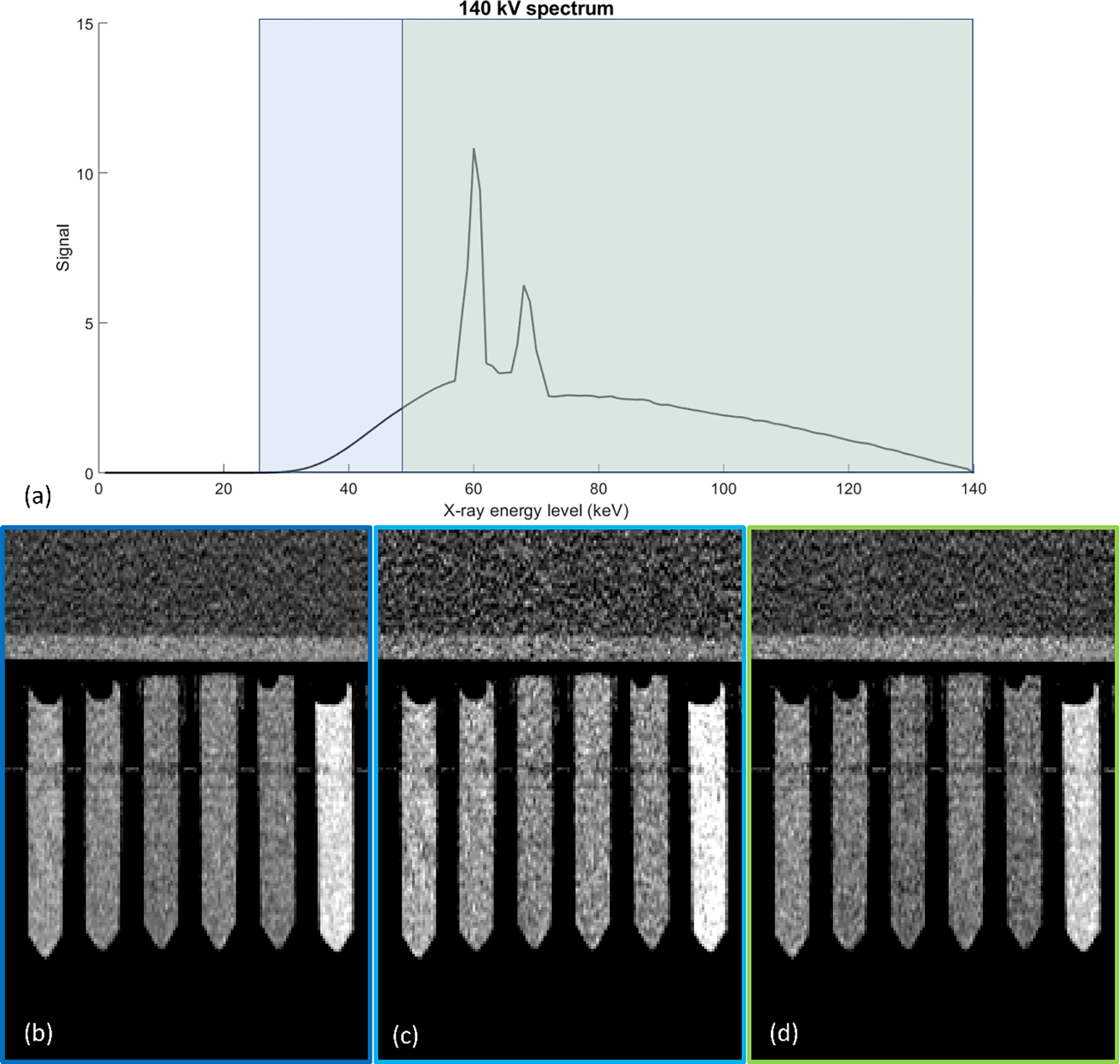
Example of energy spectrum and division into different energy selective images using photon-counting CT method. The energy spectrum (a) is divided by two energy thresholds (25 and 52 keV) into the threshold 1 region (blue and green), threshold 2 region (green). The threshold regions are subtracted to create the bin 1 (light blue) and bin 2 (green) regions. Images shown representing threshold 1 (b), bin 1 (c), and bin 2 (d). Note that threshold 2 and bin 2 images are equivalent for this acquisition setup. Vials from left to right represent: iodine 8 mg/mL, iodine 4 mg/mL, iodine 2 mg/mL, gadolinium 2 mg/mL, gadolinium 4 mg/mL, and gadolinium 8 mg/mL Images taken from 140 kV tube voltage, 150 mAs tube current, and 25–52 keV threshold case and presented with window width/window level of 200/100.
2.3. Phantom and datasets
A cylindrical water phantom (30 cm diameter, 35 cm length, 13 cm open bore, Fig. 2) was used to image vials of iodine (Isovue 300, Bracco Diagnostics Inc., Monroe Township, NJ) and gadolinium (ProHance, Bracco Diagnostics) at three concentration levels (2, 4, 8 mg/mL). Images were acquired with multiple tube current, tube voltage, and high energy threshold values (Table 1). The range of possible values for the high energy threshold was dependent on the choice of tube current. The low energy threshold was fixed at 25 keV. Each scan was repeated three times. Reconstruction was done on a vendor provided off-line reconstruction machine (ReconCT v. 14.0.1.39923, Siemens) using filtered backprojection with a D40f kernel and 1.0 mm slice thickness.
Figure 2 –

Image of the phantom used in this study (left). Reconstructed image (right) showing examples of regions-of-interest drawn for a contrast vial (blue) and water background (yellow).
Table 1 –
Acquisition parameters for experimental data acquisition in this study
| Tube Voltage (kV) | Low energy fixed threshold (keV) | High energy variable threshold (keV) | Tube Current (mAs) |
|---|---|---|---|
| 100 | 25 | 52, 65, 80 | 50, 100, 150 |
| 120 | 25 | 52, 70, 90 | 50, 100, 150 |
| 140 | 25 | 52, 75, 90 | 50, 100, 150 |
2.4. Regions of interest and analysis
For signal measurements, three-dimensional ROIs were drawn within each vial (Fig. 2) and extracted for calculations. ROI dimensions were chosen to match the size of the vials consistently across acquisitions. Three additional ROIs (Fig. 2) were drawn in the water regions of the phantom and used as reference for background. For each signal ROI that was extracted and each noise ROI, a multivariate CNR was calculated. Since each of the datasets had two energy selective images, low and high energy, the output was a 2×2 matrix with four terms for each condition: CNRlo, CNRhi, Covar-CNRlo, and Covar-CNRhi.
The relationship between Covar-CNR and conventional CNR terms was evaluated by grouping all ROIs containing only one contrast agent based on their conventional CNR values, CNRlo, CNRhi. A sliding cutoff was applied from 0 to 10 in steps of 0.1, separating the dataset into three groups: those cases where both conventional CNR values were above the cutoff, cases where either CNRlo or CNRhi was above the cutoff, and cases where both CNR values were below the cutoff. The CNR values of 5 and 2.5, derived from the Rose criterion (Rose, 2013; Bushberg and Boone, 2011) and half of its value, were used as reference levels. The dependence of each of the four terms in the CNR matrix on acquisition parameters, including tube current, tube voltage, and energy threshold, was then evaluated for each vial.
2.5. Statistics
All statistical analysis was completed using MATLAB (v2021a, MathWorks, Natick, MA). Each component of the matrix (CNRlo, CNRhi, Covar-CNRlo, and Covar-CNRhi) was evaluated as both separate and grouped variables. Spectral CNRs for iodine and gadolinium were analyzed separately. The correlation between each pair of the four matrix components was calculated for both iodine and gadolinium.
A five-way analysis of variance (ANOVA) was calculated for each of the four matrix terms with image type, tube current, tube voltage, higher energy threshold, and material concentration as covariates. A p-value adjustment was applied to each covariate using a Holm-Bonferroni correction (Holm, 1979). Normality was evaluated using the Shapiro-Wilk test (Ben Saida, 2014). Finally, a multivariate regression was fit to the data given by the equation
| (7) |
where is the response matrix, is the number of variates in the model, is the number of observations, is a design matrix, is the number of predictors, is a vector of coefficients for the regression, and is an error term.
3. Results
3.1. Relationship between Covar-CNR and CNR terms
As the CNR cutoff value was increased, the number of cases that fell into each group decreased at a similar rate for both threshold and bin images (Fig. 3). For the reference value of 2.5, 48.5% and 52.5% of cases had both values above the cutoff, 36.4% and 33.1% had at least one value above the cutoff, and 15.0% and 14.3% had both values below the cutoff for threshold and bin cases, respectively. At the reference value of 5, 75.0% and 80.2% of cases had both values above the cutoff, 21.8% and 16.7% had at least one value above the cutoff, and 3.1% and 3.1% had both values below the cutoff for threshold and bin cases, respectively.
Figure 3 –

Percentage of cases (y-axis) that fell under each group as CNR cutoff (x-axis) was increased for threshold images (left) and bin images (right). Groups represented by different colors (both CNRs above cutoff – blue, one CNR above cutoff – red, both CNRs below cutoff – yellow). Dashed lines represent reference CNR values of 2.5 and 5.
While the number of cases that fell into each group was consistent between threshold and bin images, the mean and standard deviation of Covar-CNR cases (Fig. 4) was higher for bin images (Covar-CNRlo: 3.38 ±17.25, Covar-CNRhi: 5.77±30.64) than threshold images (Covar-CNRlo: 2.08 ±1.89, Covar-CNRhi: 3.45±2.49). As the cutoff was raised, the mean value of the Covar-CNRlo and Covar-CNRhi for cases that had one or more CNRs above the cutoff increased while the mean value for cases that fell below the cutoff increased more modestly.
Figure 4 -.
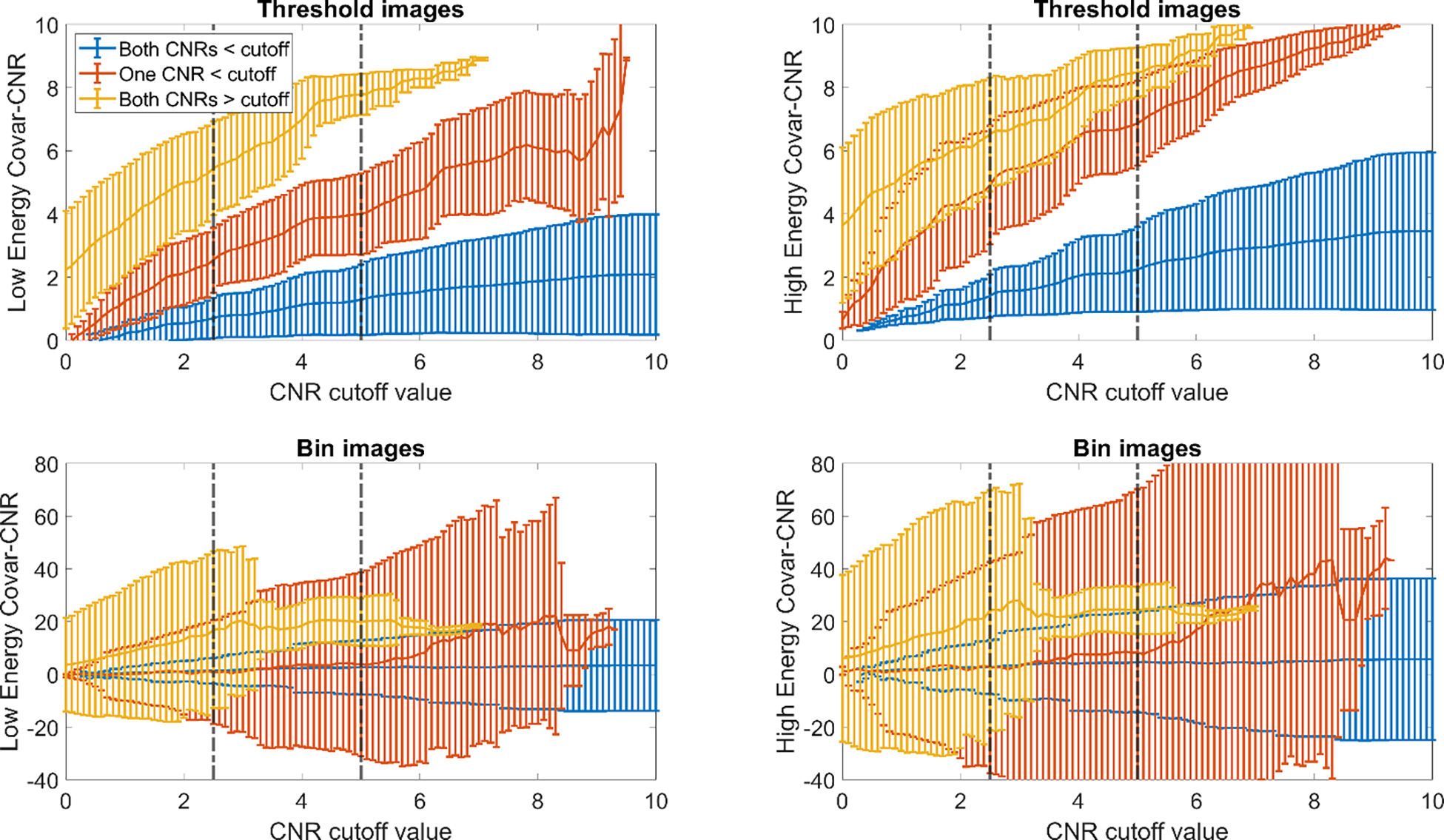
Spread of Covar-CNR terms (y-axis) for each group as CNR cutoff (x-axis) was increased. Figures separated by image type (threshold – top row, bin – bottom row) and energy level (low energy – left column, high energy – right column). Groups represented by different colors (both CNRs above cutoff – blue, one CNR above cutoff – red, both CNRs below cutoff – yellow). Values represented by the mean ± standard deviation at each cutoff point. Dashed lines represent reference CNR values of 2.5 and 5.
3.2. Characterization of acquisition parameters
CNR terms showed similar relationships for both iodine and gadolinium datasets as different acquisition variables were changed. While CNRlo and CNRhi were comparable between bin and threshold images, Covar-CNRlo and Covar-CNRhi had a larger magnitude for binned images across most conditions.
For binned images and a fixed tube voltage, increase in energy threshold led to an increase in CNRlo, decrease in CNRhi, and variable change in Covar-CNR terms (Fig. 5). For threshold images with a fixed tube voltage, increase in energy threshold had a similar effect on CNRlo, CNRhi, and Covar-CNRhi terms, while Covar-CNRlo decreased with energy threshold. When energy threshold is held fixed and tube voltage is increased for binned images, CNRlo and CNRhi increased while Covar-CNRlo and Covar-CNRhi decreased (Fig. 6). There was a more dramatic decrease from 100kV to 120kV than between 120kV and 140kV. For threshold images with a fixed energy threshold and increasing tube voltage, CNRlo increased with tube voltage, while CNRhi, Covar-CNRlo, and Covar-CNRhi reached a peak at 120kV. When image type, tube voltage, and energy threshold are held fixed, all CNR terms increased with tube current and material concentrations for both iodine (Fig. 7) and gadolinium (Fig. 8).
Figure 5 –

CNR measures for binned images with a fixed 100 kV tube voltage and variable energy threshold (x-axis). Measures represented by CNR (top row) and Covar-CNR (bottom row) and separated by energy level (low energy – left, high energy – right). Concentrations for iodine (blue) and gadolinium (green) indicated by increasing shade.
Figure 6 –

CNR measures for binned images with a fixed energy threshold (52 keV) and variable tube voltage (x-axis). Measures represented by CNR (top row) and Covar-CNR (bottom row) and separated by energy level (low energy – left, high energy – right). Concentrations for iodine (blue) and gadolinium (green) indicated by increasing shade.
Figure 7 –

Heatmaps of iodine CNR terms for fixed tube voltage (120 kV), energy threshold (52 keV), and image type (bin) as a function of tube current (x-axis) and material concentration (y-axis). Measures represented by CNR (top row) and Covar-CNR (bottom row) and separated by energy level (low energy – left, high energy – right).
Figure 8 –

Heatmaps of gadolinium CNR terms for fixed tube voltage (120 kV), energy threshold (52 keV), and image type (bin) as a function of tube current (x-axis) and material concentration (y-axis). Measures represented by CNR (top row) and Covar-CNR (bottom row) and separated by energy level (low energy – left, high energy – right).
3.3. Statistical modelling
Correlations were highest for the CNRlo/CNRhi and Covar-CNRlo/Covar-CNRhi pairs for both iodine and gadolinium (Fig. 9). For both iodine and gadolinium datasets, the Shaprio-Wilk test showed that each CNR and Covar-CNR term was highly normal (p <0.01).
Figure 9 -.

Correlation matrices between each of the multivariate CNR matrix terms (CNRlo, Covar-CNRlo, CNRhi, Covar-CNRhi) for iodine (left) and gadolinium (right). Lighter shade of blue indicates a lower correlation between each pair.
The results of the five-way analysis of variance for main effects are summarized for iodine and gadolinium datasets (Table 2) for each of the four outcomes. Most p-values were small (<0.05) and thus results were statistically significant for most combinations of CNR term and covariate. For both datasets, high p-values (p > 0,05) were found for three combinations: CNRlo with energy threshold, CNRhi with image type, and Covar-CNRlo with tube voltage. For iodine only, the additional combinations of CNRlo with tube voltage and Covar-CNRlo with image type had higher p-values.
Table 2 –
Summary of N-way analysis of variance for iodine and gadolinium datasets for each CNR measure. P-values were adjusted using the Holm-Bonferroni correction.
| Iodine | ||||||||||
|---|---|---|---|---|---|---|---|---|---|---|
| Image Type | Tube Voltage | Tube Current | Energy Threshold | Iodine Concentration | ||||||
| F-statistic | P-value | F-statistic | P-value | F-statistic | P-value | F-statistic | P-value | F-statistic | P-value | |
| CNRlo | 28.46 | 0.00 | 4.23 | 0.08 | 1442.35 | 0.00 | 1.58 | 0.21 | 19773.02 | 0.00 |
| CNRhi | 0.81 | 0.37 | 27.00 | 0.00 | 126.03 | 0.00 | 2042.72 | 0.00 | 2914.65 | 0.00 |
| Covar-CNRlo | 3.45 | 0.08 | 4.30 | 0.08 | 8.14 | 0.01 | 61.64 | 0.00 | 38.89 | 0.00 |
| Covar-CNRhi | 5.48 | 0.02 | 12.74 | 0.01 | 13.63 | 0.01 | 17.77 | 0.00 | 17.87 | 0.00 |
| Gadolinium | ||||||||||
| Image Type | Tube Voltage | Tube Current | Energy Threshold | Gadolinium Concentration | ||||||
| F-statistic | P-value | F-statistic | P-value | F-statistic | P-value | F-statistic | P-value | F-statistic | P-value | |
| CNRlo | 167.88 | 0.00 | 79.37 | 0.00 | 1614.31 | 0.00 | 42.96 | 0.77 | 17613.36 | 0.00 |
| CNRhi | 0.39 | 0.53 | 105.32 | 0.00 | 256.84 | 0.00 | 2908.91 | 0.00 | 3250.21 | 0.00 |
| Covar-CNRlo | 5.88 | 0.03 | 1.16 | 0.28 | 24.80 | 0.00 | 45.48 | 0.00 | 38.94 | 0.00 |
| Covar-CNRhi | 3.83 | 0.05 | 4.97 | 0.05 | 26.65 | 0.00 | 14.39 | 0.00 | 27.64 | 0.00 |
Multivariate regressions for iodine and gadolinium (Table 3) are summarized. The intercept terms for iodine were closer to zero than gadolinium for all four matrix terms, with the CNRlo and Covar-CNRhi intercepts being negatively valued. Coefficients had identical signs for both iodine and gadolinium datasets. The multi-dimensional outcome of the four CNR variables increased slightly with tube current and tube voltage and more dramatically with material concentration. An increase in energy threshold increased the CNRlo term only. The image type term, which acts as an adjustment for bin images, results in a lower intercept term for CNRlo and Covar-CNRlo and a higher intercept term for CNRhi and Covar-CNRhi.
Table 3 –
Summary of multivariate regression fit (intercept and slopes) for iodine and gadolinium datasets for each CNR measure. Associated p-values listed in parentheses.
| Iodine | CNRlo | CNRhi | Covar-CNRlo | Covar-CNRhi |
|---|---|---|---|---|
| Intercept | −2.040 (0,00) | 2.214 (0.21) | 1.479 (0.00) | −7.633 (0.05) |
| Tube Voltage | 0.002 (0.04) | 0.026 (0.04) | 0.004 (0.00) | 0.100 (0.00) |
| Tube Current | 0.011 (0.00) | 0.014 (0.00) | 0.003 (0.00) | 0.040 (0.00) |
| Energy Threshold | 0.001 (0.21) | −0.110 (0.00) | −0.038 (0.00) | −0.131 (0.00) |
| Material Concentration | 0.692 (0.00) | 0.501 (0.00) | 0.264 (0.00) | 0.759 (0.00) |
| Image Type | −0.131 (0.00) | 0.746 (0.06) | −0.022 (0.37) | 2.095 (0.02) |
| Gadolinium | CNRlo | CNRhi | Covar-CNRlo | Covar-CNRhi |
| Intercept | −3.531 (0.00) | 3.028 (0.38) | 2.258 (0.00) | −9.333 (0.10) |
| Tube Voltage | 0.009 (0.00) | 0.026 (0.28) | 0.011 (0.00) | 0.090 (0.03) |
| Tube Current | 0.016 (0.00) | 0.047 (0.00) | 0.007 (0.00) | 0.082 (0.00) |
| Energy Threshold | 0.008 (0.00) | −0.183 (0.00) | −0.066 (0.00) | −0.171 (0.00) |
| Material Concentration | 0.886 (0.00) | 0.973 (0.00) | 0.399 (0.00) | 1.367 (0.00) |
| Image Type | −0.431 (0.00) | 1.886 (0.02) | −0.022 (0.53) | 2.537 (0.05) |
4. Discussion
Spectral CT is a development from conventional CT that introduces an additional dimension of information. Since multiple energies are acquired simultaneously, energy selective images cannot be treated as independent of one another like conventional CT images can be. Conventional image quality metrics, which we use to evaluate the performance of CT systems and identify which conditions produce the best clinical outcomes, are inadequate to assess the totality of spectral CT data as these metrics assume independence of images that they evaluate and do not account for the impact of shared information on signal within an image. In this work, we developed a metrology that allows for the characterization of the shared nature of energy selective images while retaining the comparative benefits of conventional imaging metrics.
We model information in a CT image by extending a conventional univariate model into a multivariate one that groups multiple images into one data structure and enables the inclusion of interaction of information between images in the dataset. Applying this model definition to the conventional signal-to-noise ratio (SNR) model to define a matrix form multivariate SNR provides a method that enables two forms of characterization. First, the inherent signal and noise properties of each image are characterized by the conventional SNR terms of the matrix. Second, the impact of shared information between the signal and noise of each image is characterized by the covariance weighted terms. By addressing both aspects of information within a spectral CT dataset, this metrology was able to characterize the interactions of information between images better than conventional metrics.
In this work, we defined the functional form of signal within the multivariate SNR framework as contrast and thus evaluated the multivariate contrast-to-noise ratio (CNR) of spectral CT image data. While change in CNR value due to change in tube current, tube voltage, and similar acquisition parameters is well documented and repeated in our experimental data, the Covar-CNR provides an understanding of how those parameters affect the relationship between signal in an image and the shared component of signal between low and high energy images. For parameters that do not impact the underlying signal distribution, Covar-CNR behaves similarly to conventional CNR. For example, increasing tube current leads to an increase in photons that are being successfully detected and thus reduces uncertainty in signal, but has a limited impact on the signal distribution which leads to an increase in both conventional and Covar-CNR.
For variables that impact the distribution or content of the signal, Covar-CNR is able to provide a more truthful characterization than conventional CNR. Increasing tube voltage leads to an increase in higher energy photons in the pre-attenuated x-ray spectrum. These photons are less likely to be attenuated than low energy photons and thus more are detected. The net effect was a decrease in contrast and noise. Since the magnitude of noise reduction was greater than contrast reduction, conventional CNR would suggest that this is an improvement in image quality. However, due to the shift in the x-ray spectrum, covariance between both low and high energy images was also increased with tube voltage which was captured as a reduction in Covar-CNR.
Image type also had a strong influence on the distribution of signal between low and high energy images and was responsible for the largest difference between CNR and Covar-CNR values. By construction, threshold and bin images have different distributions of signal as threshold images contain the signal between thresholds and the max value while bin images contain the signal between thresholds (Yu et al., 2016b; Rajagopal et al., 2019). This causes two major differences between the two image types. First, low energy bin and threshold images have different amounts and kinds of signal as the threshold image includes more high energy photons. This causes the low threshold image to have lower noise as there are more total photons in that image. However, the signal in the lower bin image is more representative of low energy photons which carry more contrast information. As a result, threshold images had a higher conventional CNR than binned images due to the decrease in noise. The second difference between threshold and binned images concerns the relationship between signals in low and high images. There is a higher correlation between signal in low and high threshold images than bin images as the entire signal of the high threshold image is contained within the low energy threshold image. As a result, binned images had higher Covar-CNRs by an order of magnitude. While conventional CNR would suggest that the threshold images had superior image quality, for applications that would require both low and high energy images, the binned image pair would provide better performance due lower covariance and thus higher Covar-CNRs. These effects were reflected in the ANOVA results, where the only term without a significant relationship with image type was CNRhi. CNRlo changed between threshold and image type due to the first difference outlined while both Covar-CNR terms were impacted by the second difference.
While the metrology developed in this work was focused on the covariance between energy selective images, image quality in individual CT images can be affected by other correlations. Two sources of this correlation can include the correlation between image pixels which originate from the same projection and correlation between adjacent slices which have highly similar signals. These correlations are incorporated into other image quality metrologies (Samei et al., 2019). For example, both the Z-axis task transfer function and 3D task transfer function (Robins et al., 2018) incorporate slice-to-slice correlation by evaluating resolution along the slice dimension. Ensemble metrologies, such as noise uniformity and noise stationarity (Solomon et al., 2020), are able to account for pixel-to-pixel correlation. Using these techniques in concert with multivariate CNR can result in a more robust evaluation of spectral CT acquisitions.
There have been earlier evaluations of PCCT systems examining the relationship between CNR and acquisition variables. Gutjahr et al. (Gutjahr et al., 2016) looked at the impact of changing tube voltage on CNR in a series of anthropomorphic phantoms and cadaver images. They found that noise decreased with increasing tube voltage and tube current and as a result CNR increased similarly. Rajagopal et al. (Rajagopal et al., 2020) characterized the CNR relationship for changing tube currents and similarly found that increasing tube current reduced noise and improved CNR. Finally, in a different study, Rajagopal et al. (Rajagopal et al., 2019) examined the impact of changing energy threshold on conventional image quality metrics including CNR and found that increasing energy threshold led to a decrease in CNR for high energy images and increased CNR in low energy bin images. Our conventional CNR findings reflect these relationships as well.
While the covariance between energy selective images has not been extensively evaluated as a measure of image quality, it has been implicitly used within multiple post-processing frameworks. Notably, the covariance between energy selective images has been exploited for denoising (Kalender et al., 1988; Petrongolo et al., 2015) and material decomposition applications (Niu et al., 2014; Schirra et al., 2014). The covariance matrix has been used to reduce overlap in information between different images to better produce denoised images or material maps. Instead of using this information for an image processing outcome, our work uses the same information as a method of characterization within the multivariate SNR framework. While the understanding of these relationships was implicit in image processing applications in the past, we sought to include the covariance in our understanding of system function due to change in acquisition and physical parameters.
When designing clinical protocols for specific tasks, the choice of parameters effects the signal in acquired images. Thus, understanding the relationship between image acquisition conditions and resulting signal helps to optimally design task-specific protocols. With the transition from conventional to spectral CT, protocol design becomes more complex with the relationship between multiple images. By both assessing each of the images individually and incorporating the covariance between multiple images, the multivariate CNR evaluates the overall landscape holistically: the multivariate CNR can be used to minimize the covariance between images while maximizing image quality within each image. Acquired images can be furthered tuned for the needs of specific clinical tasks.
There are some limitations to our work. First, the experimental dataset used in this paper was limited to the two-energy case and photon-counting CT acquisitions. Future evaluations will expand to consider multi-energy datasets, other methods of spectral CT acquisition, and other information processing variations including iterative reconstruction and post-processed images. Second, contrast is one example of a signal model. The multivariate model can be expanded to other signal estimations, for example, the ratio of mean signal between two image types, to evaluate different considerations of signal representation.
Conclusions
With the development of spectral CT techniques that acquire images at multiple energy levels, image quality metrics must also adapt to properly characterize energy selective images. Conventional metrics are limited in this capacity by the assumption of independence between images and the inability to account for shared information. In this work, we described a theoretical framework to extend the signal-to-noise ratio to a multivariate form that is able to characterize images independently and also provide insight regarding the relationship between images. Experimental data were used to demonstrate the insight that this metrology can provide regarding image formation factors in spectral CT including the distribution of photons between low and high energy images.
Acknowledgement
The authors would like to thank Dr. Nusrat Rabbee for statistical consultation. This study was supported in part by the NIH Graduate Partnership Program and the NIH (P41EB028744). The content of this manuscript does not necessarily reflect the views or policies of the Department of Health and Human Services, nor do mention of trade names, commercial products, or organizations imply endorsement by the United States Government.
Footnotes
Conflicts of interest
Author PS is an employee of Siemens Healthineers. Author ES lists relationships with the following entities unrelated to the present publication: GE, Bracco, Imalogix, 12Sigma, Metis Health Analytics, Cambridge University Press, and Wiley and Sons.
References
- Agostini A, Borgheresi A, Mari A, Floridi C, Bruno F, Carotti M, Schicchi N, Barile A, Maggi S and Giovagnoni A 2019. Dual-energy CT: theoretical principles and clinical applications La radiologia medica 124 1281–95 [DOI] [PubMed] [Google Scholar]
- Alvarez RE and Macovski A 1976. Energy-selective reconstructions in x-ray computerised tomography Physics in Medicine & Biology 21 733. [DOI] [PubMed] [Google Scholar]
- Ben Saida A 2014. Shapiro-Wilk and Shapiro-Francia normality tests.: MATLAB Central File Exchange; ) [Google Scholar]
- Bushberg JT and Boone JM 2011. The essential physics of medical imaging: Lippincott Williams & Wilkins; ) [Google Scholar]
- Dabli D, Loisy M, Frandon J, de Oliveira F, Meerun AM, Guiu B, Beregi J-P and Greffier J 2023. Comparison of image quality of two versions of deep-learning image reconstruction algorithm on a rapid kV-switching CT: A phantom study European Radiology Experimental 7 1. [DOI] [PMC free article] [PubMed] [Google Scholar]
- Euler A, Parakh A, Falkowski AL, Manneck S, Dashti D, Krauss B, Szucs-Farkas Z and Schindera ST 2016. Initial results of a single-source dual-energy computed tomography technique using a split-filter: assessment of image quality, radiation dose, and accuracy of dual-energy applications in an in vitro and in vivo study Investigative radiology 51 491–8 [DOI] [PubMed] [Google Scholar]
- Farhadi F, Rajagopal JR, Nikpanah M, Sahbaee P, Malayeri AA, Pritchard WF, Samei E, Jones EC and Chen MY 2021. Review of Technical Advancements and Clinical Applications of Photon-counting Computed Tomography in Imaging of the Thorax Journal of Thoracic Imaging 36 84–94 [DOI] [PubMed] [Google Scholar]
- Flohr T and Schmidt B 2023. Technical basics and clinical benefits of photon-counting CT Investigative Radiology 58 441–50 [DOI] [PMC free article] [PubMed] [Google Scholar]
- Greffier J, Pastor M, Si-Mohamed S, Goutain-Majorel C, Peudon-Balas A, Bensalah MZ, Frandon J, Beregi J-P and Dabli D 2024. Comparison of two deep-learning image reconstruction algorithms on cardiac CT images: A phantom study Diagnostic and Interventional Imaging 105 110–7 [DOI] [PubMed] [Google Scholar]
- Greffier J, Si-Mohamed SA, Lacombe H, Labour J, Djabli D, Boccalini S, Varasteh M, Villien M, Yagil Y and Erhard K 2023a. Virtual monochromatic images for coronary artery imaging with a spectral photon-counting CT in comparison to dual-layer CT systems: a phantom and a preliminary human study European Radiology 33 5476–88 [DOI] [PMC free article] [PubMed] [Google Scholar]
- Greffier J, Van Ngoc Ty C, Fitton I, Frandon J, Beregi J-P and Dabli D 2023b. Impact of Phantom Size on Low-Energy Virtual Monoenergetic Images of Three Dual-Energy CT Platforms Diagnostics 13 3039. [DOI] [PMC free article] [PubMed] [Google Scholar]
- Gutjahr R, Halaweish AF, Yu Z, Leng S, Yu L, Li Z, Jorgensen SM, Ritman EL, Kappler S and McCollough CH 2016. Human imaging with photon-counting-based CT at clinical dose levels: Contrast-to-noise ratio and cadaver studies Investigative Radiology 51 421. [DOI] [PMC free article] [PubMed] [Google Scholar]
- Higaki T, Nakamura Y, Zhou J, Yu Z, Nemoto T, Tatsugami F and Awai K 2020. Deep learning reconstruction at CT: phantom study of the image characteristics Academic radiology 27 82–7 [DOI] [PubMed] [Google Scholar]
- Holm S 1979. A simple sequentially rejective multiple test procedure Scandinavian journal of statistics 65–70 [Google Scholar]
- Johnson TR 2012. Dual-energy CT: general principles American Journal of Roentgenology 199 S3–S8 [DOI] [PubMed] [Google Scholar]
- Johnston A, Mahesh M, Uneri A, Rypinski TA, Boone JM and Siewerdsen JH 2024. Objective image quality assurance in cone-beam CT: Test methods, analysis, and workflow in longitudinal studies Medical Physics [DOI] [PubMed] [Google Scholar]
- Kalender WA, Klotz E and Kostaridou L 1988. An algorithm for noise suppression in dual energy CT material density images IEEE transactions on medical imaging 7 218–24 [DOI] [PubMed] [Google Scholar]
- Kappler S, Glasser F, Janssen S, Kraft E and Reinwand M Medical Imaging 2010: Physics of Medical Imaging,2010), vol. Series 7622): International Society for Optics and Photonics; ) p 76221Z [Google Scholar]
- Kawashima H, Ichikawa K, Ueta H, Takata T, Mitsui W and Nagata H 2023. Virtual monochromatic images of dual-energy CT as an alternative to single-energy CT: performance comparison using a detectability index for different acquisition techniques European Radiology 33 5752–60 [DOI] [PubMed] [Google Scholar]
- Kreul DA, Kubik-Huch RA, Froehlich J, Thali MJ and Niemann T 2021. Spectral Properties of Abdominal Tissues on Dual-energy Computed Tomography and the Effects of Contrast Agent in vivo 35 3277–87 [DOI] [PMC free article] [PubMed] [Google Scholar]
- Marin D, Boll DT, Mileto A and Nelson RC 2014. State of the art: dual-energy CT of the abdomen Radiology 271 327–42 [DOI] [PubMed] [Google Scholar]
- McCollough CH, Boedeker K, Cody D, Duan X, Flohr T, Halliburton SS, Hsieh J, Layman RR and Pelc NJ 2020. Principles and applications of multienergy CT: Report of AAPM Task Group 291 Medical physics 47 e881–e912 [DOI] [PubMed] [Google Scholar]
- Niu T, Dong X, Petrongolo M and Zhu L 2014. Iterative image-domain decomposition for dual-energy CT Medical physics 41 041901. [DOI] [PubMed] [Google Scholar]
- Parakh A, Lennartz S, An C, Rajiah P, Yeh BM, Simeone FJ, Sahani DV and Kambadakone AR 2021. Dual-Energy CT Images: Pearls and Pitfalls RadioGraphics 41 98–119 [DOI] [PMC free article] [PubMed] [Google Scholar]
- Petrongolo M, Dong X and Zhu L 2015. A general framework of noise suppression in material decomposition for dual-energy CT Medical physics 42 4848–62 [DOI] [PubMed] [Google Scholar]
- Primak AN, Giraldo JCR, Eusemann CD, Schmidt B, Kantor B, Fletcher JG and McCollough CH 2010. Dual-source dual-energy CT with additional tin filtration: Dose and image quality evaluation in phantoms and in-vivo AJR. American journal of roentgenology 195 1164. [DOI] [PMC free article] [PubMed] [Google Scholar]
- Rajagopal JR, Farhadi F, Negussie AH, Abadi E, Sahbaee P, Saboury B, Malayeri AA, Pritchard WF, Jones EC and Samei E Medical Imaging 2021: Physics of Medical Imaging,2021), vol. Series 11595): International Society for Optics and Photonics; ) p 115954I [Google Scholar]
- Rajagopal JR, Jones EC and Samei E Medical Imaging 2019: Physics of Medical Imaging,2019), vol. Series 10948): SPIE; ) pp 1125–32 [Google Scholar]
- Rajagopal JR, Sahbaee P, Farhadi F, Solomon JB, Ramirez-Giraldo JC, Pritchard WF, Wood BJ, Jones EC and Samei E 2020. A Clinically Driven Task-Based Comparison of Photon Counting and Conventional Energy Integrating CT for Soft Tissue, Vascular, and High-Resolution Tasks IEEE Transactions on Radiation and Plasma Medical Sciences [DOI] [PMC free article] [PubMed] [Google Scholar]
- Rajagopal JR, Schwartz FR, McCabe C, Farhadi F, Zarei M, Ria F, Abadi E, Segars P, Ramirez-Giraldo JC and Jones EC 2024. Technology Characterization Through Diverse Evaluation Methodologies: Application to Thoracic Imaging in Photon-Counting Computed Tomography Journal of Computer Assisted Tomography 10.1097 [DOI] [PMC free article] [PubMed] [Google Scholar]
- Rajiah P, Sundaram M and Subhas N 2019. Dual-energy CT in musculoskeletal imaging: what is the role beyond gout? American Journal of Roentgenology 213 493–505 [DOI] [PubMed] [Google Scholar]
- Rassouli N, Etesami M, Dhanantwari A and Rajiah P 2017. Detector-based spectral CT with a novel dual-layer technology: principles and applications Insights into imaging 8 589–98 [DOI] [PMC free article] [PubMed] [Google Scholar]
- Robins M, Solomon J, Richards T and Samei E 2018. 3D task-transfer function representation of the signal transfer properties of low-contrast lesions in FBP-and iterative-reconstructed CT Medical physics 45 4977–85 [DOI] [PubMed] [Google Scholar]
- Rose A 2013. Vision: human and electronic: Springer Science & Business Media; ) [Google Scholar]
- Samei E, Bakalyar D, Boedeker KL, Brady S, Fan J, Leng S, Myers KJ, Popescu LM, Ramirez Giraldo J C and Ranallo F 2019. Performance Evaluation of Computed Tomography Systems: Summary of AAPM Task Group 233 Medical physics [DOI] [PubMed] [Google Scholar]
- Schirra CO, Brendel B, Anastasio MA and Roessl E 2014. Spectral CT: a technology primer for contrast agent development Contrast media & molecular imaging 9 62–70 [DOI] [PubMed] [Google Scholar]
- Shikhaliev PM, Fritz SG and Chapman JW 2009. Photon counting multienergy x-ray imaging: Effect of the characteristic X rays on detector performance Medical physics 36 5107–19 [DOI] [PubMed] [Google Scholar]
- Solomon J, Lyu P, Marin D and Samei E 2020. Noise and spatial resolution properties of a commercially available deep learning-based CT reconstruction algorithm Medical physics 47 3961–71 [DOI] [PubMed] [Google Scholar]
- Taguchi K, Stierstorfer K, Polster C, Lee O and Kappler S 2018a. Spatio-energetic cross-talk in photon counting detectors: N× N binning and sub-pixel masking Medical physics 45 4822–43 [DOI] [PubMed] [Google Scholar]
- Taguchi K, Stierstorfer K, Polster C, Lee O and Kappler S 2018b. Spatio-energetic cross-talk in photon counting detectors: Numerical detector model (Pc TK) and workflow for CT image quality assessment Medical physics 45 1985–98 [DOI] [PubMed] [Google Scholar]
- Taguchi K, Zhang M, Frey EC, Wang X, Iwanczyk JS, Nygard E, Hartsough NE, Tsui BM and Barber WC 2011. Modeling the performance of a photon counting x-ray detector for CT: Energy response and pulse pileup effects Medical physics 38 1089–102 [DOI] [PMC free article] [PubMed] [Google Scholar]
- Vrbaski S, Bache S, Rajagopal J and Samei E 2023. Quantitative performance of photon-counting CT at low dose: Virtual monochromatic imaging and iodine quantification Medical physics 50 5421–33 [DOI] [PMC free article] [PubMed] [Google Scholar]
- Wang AS, Harrison D, Lobastov V and Tkaczyk JE 2011. Pulse pileup statistics for energy discriminating photon counting x-ray detectors Medical physics 38 4265–75 [DOI] [PubMed] [Google Scholar]
- Xu C, Danielsson M and Bornefalk H 2011. Evaluation of energy loss and charge sharing in cadmium telluride detectors for photon-counting computed tomography IEEE Transactions on Nuclear Science 58 614–25 [Google Scholar]
- Xu D, Langan DA, Wu X, Pack JD, Benson TM, Tkaczky JE and Schmitz AM Medical Imaging 2009: Physics of Medical Imaging,2009), vol. Series 7258): SPIE; ) pp 1198–207 [Google Scholar]
- Yu L, Christner JA, Leng S, Wang J, Fletcher JG and McCollough CH 2011. Virtual monochromatic imaging in dual-source dual-energy CT: radiation dose and image quality Medical physics 38 6371–9 [DOI] [PMC free article] [PubMed] [Google Scholar]
- Yu L, Li Z, Leng S and McCollough CH Medical Imaging 2016: Physics of Medical Imaging,2016a), vol. Series 9783): International Society for Optics and Photonics; ) p 978312 [Google Scholar]
- Yu Z, Leng S, Jorgensen SM, Li Z, Gutjahr R, Chen B, Halaweish AF, Kappler S, Yu L and Ritman EL 2016b. Evaluation of conventional imaging performance in a research whole-body CT system with a photon-counting detector array Physics in Medicine & Biology 61 1572. [DOI] [PMC free article] [PubMed] [Google Scholar]
- Yu Z, Leng S, Li Z, Halaweish AF, Kappler S, Ritman EL and McCollough CH 2016c. How low can we go in radiation dose for the data-completion scan on a research whole-body photon-counting CT system Journal of computer assisted tomography 40 663. [DOI] [PMC free article] [PubMed] [Google Scholar]
- Zhong J, Shen H, Chen Y, Xia Y, Shi X, Lu W, Li J, Xing Y, Hu Y and Ge X 2023. Evaluation of image quality and detectability of deep learning image reconstruction (DLIR) algorithm in single-and dual-energy CT Journal of Digital Imaging 36 1390–407 [DOI] [PMC free article] [PubMed] [Google Scholar]