An Ensemble Learning Approach Based on TabNet and Machine Learning Models for Cheating Detection in Educational Tests

Abstract

The pervasive issue of cheating in educational tests has emerged as a paramount concern within the realm of education, prompting scholars to explore diverse methodologies for identifying potential transgressors. While machine learning models have been extensively investigated for this purpose, the untapped potential of TabNet, an intricate deep neural network model, remains uncharted territory. Within this study, a comprehensive evaluation and comparison of 12 base models (naive Bayes, linear discriminant analysis, Gaussian process, support vector machine, decision tree, random forest, Extreme Gradient Boosting (XGBoost), AdaBoost, logistic regression, k-nearest neighbors, multilayer perceptron, and TabNet) was undertaken to scrutinize their predictive capabilities. The area under the receiver operating characteristic curve (AUC) was employed as the performance metric for evaluation. Impressively, the findings underscored the supremacy of TabNet (AUC = 0.85) over its counterparts, signifying the profound aptitude of deep neural network models in tackling tabular tasks, such as the detection of academic dishonesty. Encouraged by these outcomes, we proceeded to synergistically amalgamate the two most efficacious models, TabNet (AUC = 0.85) and AdaBoost (AUC = 0.81), resulting in the creation of an ensemble model christened TabNet-AdaBoost (AUC = 0.92). The emergence of this novel hybrid approach exhibited considerable potential in research endeavors within this domain. Importantly, our investigation has unveiled fresh insights into the utilization of deep neural network models for the purpose of identifying cheating in educational tests.

Introduction

The perpetual quandary of identifying instances of cheating in educational tests has posed a long-standing challenge for educators. With the relentless progression of technology, the ease with which students can engage in fraudulent practices during examinations has escalated significantly. Such misconduct not only bestows an unwarranted advantage upon the cheaters but also undermines the sanctity of the testing process, thereby jeopardizing the authenticity and accuracy of the results. Consequently, the detection of cheating in educational tests assumes paramount importance, as it serves to safeguard the integrity and reputation of educational institutions while ensuring equitable and precise evaluation of candidates’ knowledge and aptitude.

Numerous endeavors have been undertaken to counteract the threat posed by cheating behavior, which can be categorized into two broad domains: those rooted in psychometric principles and those harnessing the potential of machine learning techniques (Kim et al., 2016).

Psychometric-based approaches rely on the application of statistical analyses to test scores and response patterns to uncover suspicious behaviors. These methodologies encompass the scrutiny of various factors, including the pace at which tests are completed, response patterns, and the resemblance between the responses of different students. One potential approach involves leveraging item response theory to identify anomalous response patterns that may potentially indicate cheating (Alexandron et al., 2016; Man & Harring, 2021; Meyer & Zhu, 2013; Shu et al., 2013; Wollack et al., 2015). Another method entails employing statistical models to pinpoint test-takers whose performance significantly deviates from their customary levels (Y. Chen et al., 2022; Dawson et al., 2020; Hurtz & Weiner, 2019; Meisters et al., 2022; Reiber et al., 2023).

Machine learning–based approaches leverage sophisticated algorithms and models to analyze vast data sets of test scores, thereby unveiling behavioral patterns that could signify cheating. These techniques involve training algorithms on extensive historical data sets of previous test scores and employing them to detect irregular behaviors in current test-takers. For instance, data mining methods such as k-means, Gaussian finite mixture, self-organization mapping, k-nearest neighbor, random forest, and support vector machine have been explored to identify instances of cheating in large-scale assessments (Man et al., 2019). Extreme Gradient Boosting (XGBoost) has been employed to detect examinees with preknowledge (EWP) (Zopluoglu, 2019). Classical machine learning models have been trained and compared to identify cheaters in online exams (Kadthim & Ali, 2023). Recurrent neural networks have been utilized to uncover instances of cheating in exams (Kamalov et al., 2021). An ensemble learning technique known as stacking ensemble has been employed to identify instances of cheating, with resampling techniques addressing class imbalance (Zhou & Jiao, 2023). In addition, several other ensemble learning models have been explored to flag potential cheating test-takers (Pan & Wollacka, 2021a; Santoso et al., 2021).

Nonetheless, the utilization of machine learning models is not without its limitations. Primarily, the intricate task of tuning hyperparameters can prove to be an arduous and formidable endeavor. Second, the realm of study in which machine learning models have been extensively investigated allows for only limited avenues of novel model development.

To surmount these challenges, we undertook a meticulous examination of the efficacy of TabNet (Arik & Pfister, 2021), an intricately designed deep neural network model, within the domain of cheating detection tasks. Furthermore, we ingeniously amalgamated TabNet with AdaBoost, thereby birthing an ensemble model christened TabNet-AdaBoost. Our diligent research endeavors unveiled that TabNet-AdaBoost surpassed classical machine learning models, in addition to outperforming the baseline model (Zhou & Jiao, 2023). Consequently, our study furnishes invaluable insights into the application of deep neural network models for the purpose of identifying instances of cheating.

TabNet

This section entails a comprehensive elucidation of TabNet, encapsulating its architectural design, constituent building blocks, and operational mechanics.

Architecture

The architecture of TabNet, as shown in Figure 1, synergistically integrates the advantages of deep learning and decision trees, enabling efficient handling of tabular data by seamlessly incorporating feature selection and prediction within a single framework. Extensive empirical evaluations demonstrate TabNet’s ability to achieve outstanding performance across diverse tabular data sets, consequently fostering its widespread adoption among machine learning practitioners engaged in structured data analysis (Borghini & Giannetti, 2021; Joseph et al., 2022; McDonnell et al., 2023; Wei et al., 2022; Yan et al., 2021).

Figure 1.

Architecture of TabNet. (A) TabNet Encoder, (B) TabNet Decoder, (C) Feature Transformer, and (D) Attentive Transformer.

Note. GLU = gated linear unit; FC = fully connected; BN = batch normalization.

TabNet is built upon an adapted variation of the transformer architecture (Vaswani et al., 2017), featuring an encoder and a decoder. The encoder comprises a feature transformer, an attentive transformer, and feature masking. By utilizing a split block, the processed representation is divided for the subsequent step’s attentive transformer usage and overall output. With each step, the feature selection mask offers transparent insights into the model’s functionality, allowing aggregation of masks to derive global feature importance attribution. As for the decoder, it consists of a feature transformer block at each step, further enhancing TabNet’s capabilities.

Building Blocks

The elemental constituents of both the attentive transformer and feature transformer are designated as feature blocks. These blocks comprise a sequential application of fully connected (FC) layers and batch normalization (BN), with the additional inclusion of the gated linear unit (GLU) activation layer specifically for feature transformers. The GLU activation layer allows for improved gradient flow, enabling hidden units to propagate deeper into the model while mitigating issues of exploding or vanishing gradients.

The feature transformer can be conceived as an ordered assemblage of feature blocks. It encompasses a pair of blocks that share weights across steps, thereby reducing the proliferation of parameters within the model and fostering heightened capabilities for generalization. In addition, it incorporates two blocks that are contingent upon the specific step at hand.

In the case of the attentive transformer, it amalgamates a modified rendition of the self-attention mechanism originally present in the transformer architecture. Its input is derived from the output of the feature transformer. This module adeptly acquires the ability to attend to diverse features and their interconnections, proficiently capturing intricate dependencies and discernible patterns inherent within the data. Notably, the conventional softmax function, conventionally employed in self-attention, is supplanted by the sparsemax function, which actively promotes the introduction of sparsity within attention weights. This, in turn, facilitates the selection of salient features by assigning greater weights to a diminished subset of attributes.

Workflow

The process commences with the input features undergoing processing through the feature transformer, generating initial feature representations. Subsequently, the output from the feature transformer serves as an input to the attentive transformer, responsible for selecting a subset of features to advance to the subsequent step. This iterative process is repeated for a specified number of steps. To yield final predictions, the model leverages the feature transformer outputs obtained from each decision step. In addition, the attention masks generated at each step offer valuable insights into the utilized features for prediction. By aggregating these masks, it becomes possible to discern local feature importance as well as ascertain global feature importance.

Method

Within the ensuing sections, we embark upon a comprehensive exposition of the operational mechanics intrinsic to the proposed approach. A visual representation depicting the intricacies of this methodology can be perused in Figure 2.

Figure 2.

Block Diagram of the Proposed Approach.

The initial stage encompassed the preprocessing of the data set, encompassing crucial procedures such as imputing missing values, encoding data, and scaling features. Subsequent to this preprocessing phase, feature selection techniques were employed to identify the most pertinent features to be incorporated into the base models. The base models were then trained, with diligent attention devoted to fine-tuning their hyperparameters to maximize their performance. Following this, a weighted averaging technique was implemented to form an ensemble model that amalgamated the two most outstanding base models. Finally, this ensemble model underwent rigorous validation on the test set, facilitating a comprehensive performance evaluation juxtaposed against that of a baseline model, thus culminating in a comparative analysis.

Data Set

The data set (Cizek & Wollack, 2016) is derived from an online test that computes scores based on test-takers’ responses. It has garnered substantial attention within the research domain (Man et al., 2019; Zhou & Jiao, 2023; Zopluoglu, 2019). To offer a comprehensive understanding of the data set, Table 1 presents a comprehensive summary of its notable characteristics.

Table 1.

Description of Cheating Detection Data Set.

Data set	Total test-takers	Flagged test-takers	Categorical features	Numerical features
train set	2,624	77	253	253
test set	656	17	253	253
total	3,280	94	253	253

Note. Categorical features are nominal responses and numerical features represent response time.

The original data set consists of two distinct forms, each encompassing a total of 170 multiple-choice items. Each item presents test-takers with four nominal options: A, B, C, and D. Within this set of items, 87 are common to both forms, while the remaining 83 are exclusive to each form, thereby introducing variation between the two.

For every item, the data set records the nominal responses provided by the test-takers, along with their corresponding response times. In addition, a designated column titled Flagged is included, serving as an indicator for potential instances of cheating. A value of 1 in the Flagged column signifies the presence of cheating, whereas a value of 0 signifies the absence of cheating.

After merging Form 1 and Form 2 and eliminating duplicate items, a consolidated data set was derived, featuring 3,280 test-takers and 253 distinct items. This combined data set was subsequently divided into two subsets: a train set, which encompassed 80% of the test-takers, and a test set, which comprised the remaining 20% of the test-takers.

The train set consisted of 2,624 test-takers, among which 77 individuals were identified as engaging in cheating behavior. However, the test set comprised 656 test-takers, of which 17 were flagged as potential cheaters.

Data Preprocessing

During the data preprocessing phase, a series of three key stages were undertaken: imputation, data encoding, and feature scaling.

Imputing missing values is a necessary step in building machine learning models and deep neural network models (Donders et al., 2006). Within the current data set, missing values manifest due to the fact that each test-taker had responded to only 170 of the 253 items, consequently leaving 83 items with missing values, designated as NA. In the realm of machine learning models, it is presupposed that all variables possess significance and encompass reasonable values, a presumption that becomes jeopardized in the presence of missing values.

While one straightforward approach to tackle this predicament involves discarding entire rows that contain missing values, this method proves suboptimal for small data sets such as ours. Doing so diminishes the data set’s size and heightens the susceptibility to overfitting, thus rendering it an impractical solution.

To overcome the challenge posed by missing values, we opted to replace them with zeros, effectively addressing the issue at hand. By employing this strategy, we were able to retain the original dimensions of the data set, thereby ensuring the utilization of all available data in our models. This approach enabled us to make the most of the information at hand while preserving the data set’s integrity and allowing for comprehensive analysis.

Data encoding is a crucial step in building neural network models. Categorical data, such as the nominal responses in our data set, must be converted to numerical format because many neural network models can only handle numerical data. There are two common methods for encoding categorical data: ordinal encoding and one-hot encoding (Potdar et al., 2017; Rodríguez et al., 2018; Zopluoglu, 2019). Ordinal encoding is suitable for ordinal data that can be categorized and ranked, while one-hot encoding is particularly useful for converting nominal data, which consists of nonordered categories, such as colors, names, or categories of animals, into a machine-readable format that can be used by various machine learning algorithms. To illustrate this distinction, consider the ratings of an exam, which range from A to F. Such ratings would fall under the category of ordinal data. In contrast, colors like red, blue, green, and yellow exemplify nominal data.

Given the absence of inherent rank information within the nominal responses of our data set, we resorted to employing one-hot encoding as a means of converting them into numerical data. This transformation guaranteed that the base models could effectively analyze and leverage this information. The resulting one-hot encoding of the nominal responses is visually represented in Table 2.

Table 2.

One-Hot Encoding of Nominal Responses (A, B, C, and D).

Nominal response	One-hot encoding
A	{1,0,0,0}
B	{0,1,0,0}
C	{0,0,1,0}
D	{0,0,0,1}

After one-hot encoding, each nominal response is represented by four columns: one column for each possible option (A, B, C, or D) in each item. Therefore, the 253 nominal responses in our data set were converted to a total of 1,012 columns, labeled V1 through V1012.

The response time for each item is represented by a separate column, labeled with the prefix “idur.”. For example, idur.A84 represents the response time of Item 84 in the first form, while idur.B68 represents the response time of Item 68 in the second form. Because these columns are already numerical, one-hot encoding is not necessary.

Finally, the last column in our data set, named Flagged, was not one-hot encoded because it only contains two possible values (0 and 1). One-hot encoding would not provide any benefits in this case.

Feature scaling is also a crucial preprocessing step for machine learning and neural network models (Juszczak et al., 2002; D. Li et al., 2015; Wan, 2019). For example, gradient descent, which is a core optimization algorithm in neural network models, may perform poorly if features are on different scales. In our data set, test-taker’s nominal responses are categorical features with two possible values: 0 and 1, while their response times are numerical features that range from 0 to 1,216. It is apparent that nominal responses and response times are on different scales, hence requiring feature scaling to ensure that they are on a comparable scale. To address this issue, we standardized numerical features in our data set using z-score standardization.

Feature Selection

Building machine learning and neural network models involves a critical step called feature selection (J. Li et al., 2017; Kira & Rendell, 1992; Kumar & Minz, 2014), as it helps in the following:

• Reduce overfitting: A model can become overly complex and overfit to the training data when a data set has too many features, such as the data set used in this study. This often means the model would perform poorly on new, unseen data. By reducing the number of features, feature selection can prevent overfitting and improve the model’s generalization performance.

• Improve model performance: Removing irrelevant or redundant features can improve the model’s accuracy and efficiency by reducing noise and focusing on the most informative features.

• Reduce training time: Fewer features mean less computation; therefore, feature selection can speed up the training process and make it more scalable for large data sets.

To identify the most relevant and informative features for our models, we employed a systematic feature selection process. This involved exploring three distinct sets of input features: response time only, nominal responses only, and nominal responses plus response time.

The first set, consisting of response time only, focused exclusively on numerical information. Response time can often be a crucial predictor in educational tests, as it captures the speed or duration of a particular event or action. By examining the impact of response time as the sole input feature, we aimed to assess its individual contribution to the base model’s predictive performance. This analysis allowed us to determine whether response time alone could serve as a strong indicator of possible cheating.

The second set, comprising nominal responses only, concentrated on categorical features that represent qualitative aspects of the data set. By isolating nominal responses as the sole input features, we aimed to evaluate their predictive power and discern whether the qualitative information they carry could be sufficient for accurate predictions. This examination enabled us to assess the relevance of these features in achieving optimal model performance.

The third set, which combined nominal responses and response time, aimed to leverage the strengths of both numerical and categorical information. By considering the joint impact of these features, we sought to capture the combined predictive power arising from their synergy. This combined set allowed us to investigate whether the integration of numerical and categorical information would lead to improved model performance compared with using either set of features individually.

In summary, by systematically evaluating the performance of models trained on these feature sets, we aimed to determine the most informative set that would enhance the predictive capabilities of our models.

Evaluation Metrics

There are several widely used evaluation metrics, including accuracy, precision (Powers, 2020), recall (Davis & Goadrich, 2006), F1 score (Goutte & Gaussier, 2005), and area under the receiver operating characteristic curve (AUC), that can be used to determine the performance of the proposed model.

Although accuracy is a straightforward and easy-to-understand measure, it is not adequate when the class distribution is imbalanced. As a matter of fact, our data set is heavily imbalanced as the flagged test-takers account for only 2.9% of total test-takers. Even if a naive model blindly predicts all test-takers as noncheaters, it would get an accuracy of 97.1%, which looks really good at first glance. To this end, precision and recall can be used to evaluate binary classifiers in a class-imbalanced task. However, they are indeed often in conflict with each other, meaning that improving one metric can negatively affect the other. This trade-off is known as the precision-recall trade-off. Typically, precision is prioritized when the positive class is infrequent and the expense of false positives is substantial. Conversely, recall is emphasized when the cost of false negatives is significant.

One way to balance these two metrics is to use the F1 score or AUC. In this study, AUC is chosen as the evaluation metric for clarity and ease of visualization. AUC is a graphical representation of the performance of a binary classification model, showing the trade-off between its true positive rate (TPR) and false positive rate (FPR) as the decision threshold is varied. By plotting TPR against FPR at various threshold settings, AUC provides a visual tool for evaluating and comparing the performance of different classification algorithms or models. In general, a higher AUC score indicates a better-performing model.

Base Models

Twelve base models were explored to develop an ensemble model, including TabNet, naive Bayes (Rish, 2001), linear discriminant analysis (Xanthopoulos et al., 2013), Gaussian process (Nickisch & Rasmussen, 2008), support vector machine (Hearst et al., 1998), decision tree (Song & Ying, 2015), random forest (Breiman, 2001), XGBoost (T. Chen & Guestrin, 2016), AdaBoost (Schapire, 2013), logistic regression (Kleinbaum et al., 2002), k-nearest neighbors (Peterson, 2009), and multilayer perceptron (Riedmiller & Lernen, 2014). We chose these models based on their ability to handle both categorical and numerical features and their performance on similar classification tasks.

Hyperparameter Tuning

This section discusses the process of hyperparameter tuning of base models.

A hyperparameter (Yogatama & Mann, 2014) represents a preconfigured parameter determined by users, rather than being learned by the model itself. For instance, the inclusion of the learning rate parameter in XGBoost serves as an example of a hyperparameter because it is established by the caller prior to the training process. A detailed explanation of the hyperparameters used in each base model is provided in the Supplemental File. These hyperparameters possess considerable influence over the performance of a model, and identifying the optimal values for these parameters constitutes a crucial aspect of the fine-tuning procedure. Hyperparameter tuning typically entails training multiple models with varying hyperparameter configurations and assessing their performance on a validation set. The set of hyperparameters that yields the best performance is then selected. Refer to Figure 3 for an illustrative flowchart depicting the hyperparameter tuning process.

Figure 3.

Workflow of the Hyperparameter Tuning Process.

Note. SMOTE = Synthetic Minority Oversampling Technique.

Initially, the hyperparameter space of each base model was manually defined, taking into consideration the presence of certain real-valued features. We utilized an oversampling technique called Synthetic Minority Oversampling Technique (SMOTE) to handle the class imbalance problem present in our data set (Chawla et al., 2002). Subsequently, each base model was trained using cross-validation to improve generalization performance. Finally, to evaluate the model’s performance on the test set, we retrained it using the optimal hyperparameters identified through cross-validation (Arlot & Celisse, 2010) on the train set.

There are some key points that are worth highlighting. First, grid search (LaValle et al., 2004) was used in the process of hyperparameter tuning. By automating the exhaustive search process which can be tedious to perform manually, this technique identified the best combination of hyperparameters. Specifically, grid search trained and evaluated the base model for each possible combination of hyperparameters. For instance, consider a base model with two hyperparameters, A and B, with four and three possible values, respectively. In total, there are 12 possible pairs of hyperparameters. Grid search trained the base model using each pair of (A, B) and evaluated their performance, recording the pair with the highest score as the best hyperparameters.

Second, threefold cross-validation was employed to ensure the accurate identification of optimal hyperparameters (Anguita et al., 2012). During hyperparameter tuning, it is a methodological error to compare the performance between various hyperparameter settings using the entire train set. A model trained in this way would achieve a perfect score, as it has been exposed to all samples and their corresponding labels. However, such a model would fail to generalize to unseen samples, such as those in the test set, due to overfitting. To avoid this, the test set, which comprised the remaining samples in the data set, can be used to measure the generalization capability of different hyperparameter settings. However, there is a risk of overfitting because hyperparameters can be adjusted until the model achieves a good score on the test set, thereby compromising the reliability of the evaluation results. To mitigate this issue, the data set can be divided into three subsets: a train set, a test set, and a validation set. Training occurs on the train set, hyperparameter tuning is done on the validation set, and the optimal hyperparameters are evaluated on the test set.

However, because the data set is relatively small, partitioning it into three sets would result in a small number of samples for training. To address this, cross-validation was introduced. Therefore, the data set was partitioned into two distinct subsets: the train set and the test set. The train set was then divided into threefold, where two of the folds were utilized for training and the remaining fold was designated for testing. This process was iterated 3 times in a loop. Figure 4 illustrates how it works.

Figure 4.

Grid Search With Threefold Cross-Validation.

Third, the problem of class imbalance was addressed using SMOTE which is a technique for oversampling the minority class. The data set comprises a limited number of flagged cheaters, with only a 2.9% ratio. While the best solution to this problem is acquiring more data, it is not feasible in practice. Undersampling the majority class or dropping noncheater samples would not be appropriate, as the resulting data set would be too small for machine learning models. Oversampling the minority class is therefore a viable option. However, this approach carries the risk of overfitting, as the model could learn from the same data repeatedly. To this end, SMOTE was used to avoid overfitting and its working process can be pictorially described in Figure 5.

Figure 5.

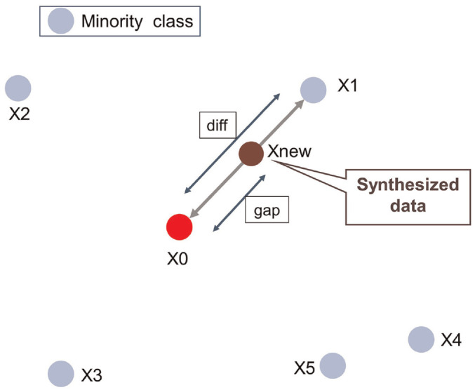
An Example Case of SMOTE to Generate a New Sample.

Note. SMOTE = Synthetic Minority Oversampling Technique.

At first, a sample that represents a cheater called X0 was randomly selected. Next, the nearest five neighbors for that sample were obtained. For the nearest neighbor X1, a feature vector called “diff” was calculated by subtracting the features of X0 from X1. Then, a random value between 0 and 1 called “gap” was multiplied by “diff” and added to X1 to create a synthesized sample which was called Xnew. This process was repeated to create synthesized samples until the number of cheaters matched that of the noncheaters.

Ensemble Models

This section discusses how ensemble models (Sagi & Rokach, 2018) are developed and how the best ensemble model is found.

First, the machine learning base models were ranked based on their performances on the test set. Next, TabNet was amalgamated with the highest-performing base model, subsequently followed by the second best-performing base model, and so on until TabNet was combined with every machine learning base model. This iterative process resulted in 11 ensemble models, each of which was named following a predefined naming convention that included the abbreviation of the corresponding base model. For instance, the ensemble model combining TabNet and naive Bayes was named TabNet-NB. Finally, the performances of all 11 ensemble models were evaluated to determine the best-performing ensemble model. Table 3 likely provides a comprehensive list of all possible names for the ensemble models, showcasing the combinations of TabNet with each machine learning base model.

Table 3.

Names of Ensemble Models Combining TabNet and the Remaining 11 Base Models.

Base model	Ensemble model
Naive Bayes	TabNet-NB
Linear discriminant analysis	TabNet-LDA
Gaussian process	TabNet-GP
Support vector machine	TabNet-SVM
Decision tree	TabNet-DT
Random forest	TabNet-RF
XGBoost	TabNet-XGB
AdaBoost	TabNet-AdaBoost
Logistic regression	TabNet-LR
K-nearest neighbors	TabNet-KNN
Multilayer perceptron	TabNet-MLP

After that, a weighted average ensemble, rather than a voting ensemble, was used when combining TabNet and machine learning base models (Sewell, 2008). The weighted average ensemble was applied following these three steps:

• Develop multiple predictive base models. To create an ensemble, we need to develop multiple base models that can make their own predictions. These base models have been described above.

• Train each model using the same training data. Once we had the base models, we trained each one on the same training data. This ensured that each base model had the same information to learn from; therefore, their predictions would be based on the same underlying patterns in the data.

• Predict using each base model and average their values with different weights. Once each base model had been trained, we used them to make predictions on new data. To combine their predictions, we took a weighted average of their predicted values. The weights assigned to each base model reflected their relative performance on a validation set or the test set. The weights could be determined using a variety of techniques, such as grid search, randomized search, or Bayesian optimization.

For example, if an ensemble has three base models with weights 0.4, 0.3, and 0.3, then the final prediction is computed as follows:

$$\begin{array}{c}\mathrm{Final}\mathrm{prediction}=0.4*\mathrm{prediction}\mathrm{from}\mathrm{base}\mathrm{model}1\hfill \\ +0.3*\mathrm{prediction}\mathrm{from}\mathrm{base}\mathrm{model}2\hfill \\ +0.3*\mathrm{prediction}\mathrm{from}\mathrm{base}\mathrm{model}3.\hfill \end{array}$$ (1)

In a weighted average ensemble, the weight assigned to each model is typically based on its performance on a validation set or through cross-validation. The better a model performs, the higher weight it is assigned, and the more impact it has on the final prediction. The weights are usually normalized to sum up to 1 to ensure that the final prediction is a proper probability distribution. Compared with a simple voting ensemble, a weighted average ensemble allows for better utilization of the strengths of each model and can lead to better overall performance. However, it requires additional effort to tune the weights for each model, and if the performance of one model significantly changes, the weights may need to be adjusted accordingly.

Ensemble methods like this pose a challenge in determining the most effective method for calculating, assigning, or searching for optimal weights that lead to better performance than any single contributing model, as well as an ensemble that distributes equal model weights. Brent’s method, which is a numerical optimization algorithm, was used to find the minimum of an objective function (Minick et al., 1988).

In the context of a weighted average ensemble, Brent’s method can be used to find the optimal weights that maximize the performance of the ensemble on a given validation set. The objective function in this case was the AUC of the ensemble on the validation set. Brent’s method started by defining an interval of weights, within which the minimum of the objective function was expected to lie. It then iteratively narrowed down the interval by finding a bracketing triplet of points that contains the minimum and can be used to construct a quadratic approximation of the objective function. The minimum of the quadratic approximation was then used as the next estimate of the minimum of the objective function, and the interval was updated accordingly. This process was repeated until the interval was small enough to provide a satisfactory estimate of the optimal weights.

Simulation Study

In the simulation study conducted to assess the effectiveness of the proposed approach, several steps were followed. These steps involved generating response data containing item preknowledge, applying the proposed approach for identifying cheaters, and analyzing the performance of the approach compared with other machine learning models. To simulate item preknowledge, the response data were initially generated and then manipulated. Four key factors were manipulated in the study: the number of items, the number of examinees, the proportion of compromised items, and the proportion of examinees with prior knowledge. These factors were combined in a full factorial design, resulting in 400 different study conditions. In addition, 16 baseline conditions that did not involve simulated prior knowledge were considered. For each condition, 30 replications were simulated independently, with compromised items and examinees with prior knowledge generated anew for each replication. The generation of normal responses and response times followed the same model and parameters as a previous study (Pan & Wollack, 2021b). The unaltered response data were then transformed to reflect item preknowledge using the same method as the aforementioned study.

The programming for the simulation study was implemented in Python 3.10, and the source code is available upon request.

Results and Discussion

This section provides a summary of the experiment results, including the feature selection outcomes, performances of the base models, performances of the ensemble models, and a comparison of our proposed model with the baseline model. In addition, the implications of our research based on the results are discussed.

Feature Selection

Three sets of input features were utilized in the training process, namely nominal responses only, response time only, and nominal responses plus response time. The objective was to determine which set of input features is most crucial for the task at hand. The performance results of these sets on the base models are presented in Table 4. The findings indicated that the response time only set of features outperformed the other two sets in eight base models, including linear discriminant analysis (AUC = 0.74), Gaussian process (AUC = 0.69), decision tree (AUC = 0.65), random forest (AUC = 0.69), XGBoost (AUC = 0.64), AdaBoost (AUC = 0.81), TabNet (AUC = 0.84), and k-nearest neighbors (AUC = 0.67). However, the nominal responses plus response time feature set achieved the highest performance in four base models, including naive Bayes (AUC = 0.72), support vector machine (AUC = 0.74), logistic regression (AUC = 0.74), and multilayer perceptron (AUC = 0.76). Notably, the nominal responses set did not attain the highest performance in any base model and exhibited the poorest performance in 11 base models, with the exception of Gaussian process (AUC = 0.64). Overall, the input feature sets that included response time demonstrated superior performance across the base models, aligning with findings from other studies (Zhou & Jiao, 2023; Zopluoglu, 2019). This could be attributed to the fact that nominal responses may not possess sufficient information to serve as effective indicators for cheating detection, unlike response time. Furthermore, considering that different base models possess distinct strengths and weaknesses, the inclusion of nominal response features may have benefited certain models while hindering others, thus explaining the inconsistent performance of the nominal responses plus response time feature set. Hence, it is crucial to carefully select and assess the relevance of input features when constructing models for cheating detection.

Table 4.

The Predictive Performance of Base Models on the Test Set Based on AUC.

Base model	Nominal responses only	Response time only	Nominal responses plus response time
Naive Bayes	0.63	0.70	0.72
Linear discriminant analysis	0.58	0.74	0.59
Gaussian process	0.64	0.69	0.61
Support vector machine	0.57	0.72	0.77
Decision tree	0.56	0.65	0.61
Random forest	0.56	0.69	0.59
XGBoost	0.56	0.64	0.59
AdaBoost	0.55	0.81	0.64
Logistic regression	0.55	0.73	0.74
TabNet	0.69	0.85	0.83
K-nearest neighbors	0.64	0.67	0.54
Multilayer perceptron	0.55	0.70	0.76

Note. AUC = area under the receiver operating characteristic curve.

Optimal Hyperparameters

The train set underwent a hyperparameter tuning process using grid search in combination with threefold cross-validation, accompanied by SMOTE to address the class imbalance issue. The results of this process are presented in Table 5, showcasing the optimal hyperparameters identified for each base model. The optimal values are highlighted in bold.

Table 5.

Hyperparameter Spaces of the Base Models and the Optimal Hyperparameters Found by Grid Search.

Base model			Hyperparameter space
Naive Bayes	var_smoothing [l,le-1,le-2,le-3,le-4,le-5,le-6,le-7,le-8,le-9]
Linear discriminant analysis	solver [‘svd’, ‘lsqr’, ‘eigen’]
Gaussian process	kernel [1*RBF(), l*DotProduct(), l*Matern(), l*RationalQuadratic(), 1 *WhiteKernel()]
Support vector machine	kernel [‘rbf, ‘poly’, ‘sigmoid’, ‘linear’]		degree [1,2,3,4,5,6]		C [0.001,0.01,0.1, 1]
Decision tree	max_features [‘auto’, ‘sqrt’, ‘log2’]		ccp_alpha [0.1,0.01,0.001]		max_depth [5,6,7,8,9]
Random forest	max_.features [‘auto’, ‘sqrt’, ‘log2’]		n_estimators [1,10, 30,100, 200]		max_depth [5,6,7,8,9]
XGBoost	learning _rate [0.05,0.10,0.15]	max_depth [8, 10, 12, 15]	min_child_weight [5,7,9, 11]	gamma [0.0,0.1,0.2,0.3,0.4]	colsample_bytree [0.4, 0.5, 0.7, 1.0]
AdaBoost	learning _rate [0.1,1,10]	n_estimators [10,100,200]	algorithm [‘SAMME’,‘SAMME.R’]
Logistic regression	solver [ ‘lbfgs’, ‘newton-cg’, ‘liblinear’, ‘sag’, ‘saga’ ]		penalty [‘11’, ‘12’, ‘elasticnet’, ‘none’]	max_iter [100, 1000, 2000]	C [0.1,0.2,0.3,0.4,0.5]
TabNet			N/A
K-nearest neighbors	n_neighbors [1,2,3,4,5,6,7,8,9,10]		weights [‘uniform’, ‘distance’]
Multilayer perceptron	hidden_layer_sizes [(10,30,10),(10,),(10,30)]	solver [‘lbfgs’, ‘sgd’, ‘adam’]	activation [‘tanh’, ‘relu’]	learning_rate [‘constant’, adaptive’, ‘invscaling’]	alpha [0.02, 0.1, 1]

For example, considering the hyperparameter tuning for AdaBoost, the following hyperparameters were tuned: learning rate, n estimators, and algorithm. For each hyperparameter, a range of values was explored: learning_rate (0.1, 1, 10), n_estimators (10, 100, 200), and algorithm (“SAMME,”‘SAMME.R’). After conducting the hyperparameter search, the best combination was determined to be learning_rate = 1, n_estimators = 100, and algorithm = ‘SAMME.’

It is important to highlight that TabNet did not undergo a hyperparameter tuning process because it was already a fine-tuned model. However, the other 11 base models required fine-tuning as their default hyperparameters did not yield desirable performances. Because each base model has its unique hyperparameter space, it is challenging to draw a common conclusion applicable to all the base models.

Performances of Base Models

The test set was utilized to make predictions using the optimal hyperparameters for each base model, enabling an assessment of their generalization capabilities. Figure 6 in the article showcases the performances of the base models.

Figure 6.

Performance Comparison of Base Models on the Test Set Based on AUC.

Note. AUC = area under the receiver operating characteristic curve.

TabNet (AUC = 0.85) exhibited superior performance compared with all the machine learning base models, regardless of the input feature set employed. This can be attributed to TabNet’s utilization of a deep neural network architecture coupled with a sparse attention mechanism, enabling the efficient fusion of information from both numerical and categorical features. This characteristic renders TabNet a potent tool for handling complex data sets encompassing mixed data types. Moreover, its distinctive architecture contributes to faster training times in comparison with other deep learning models, which is particularly advantageous for larger data sets. Furthermore, TabNet’s user-friendliness, as it does not necessitate extensive hyperparameter tuning, adds to its appeal. The combination of its impressive performance and ease of use solidifies TabNet’s significance in tasks of this nature.

However, it is important to note that although TabNet performed exceptionally well on the data set used in this study, it does not necessarily imply that deep neural network models inherently outperform machine learning models in all similar tasks. For instance, the multilayer perceptron (AUC = 0.70) occupied a middle ground in terms of performance among the models evaluated. Similarly, gradient-based boosting models faced a similar scenario, with AdaBoost ranking just behind TabNet, while XGBoost displayed the weakest performance. This indicates that both deep neural network models and gradient boosting models are not universally applicable solutions for addressing the task under investigation.

Performances of Ensemble Models

TabNet was combined with the remaining base models iteratively using the weighted average ensemble technique to achieve better performances. Figure 7 shows the performances of all 11 ensemble models.

Figure 7.

Performance Comparison of the Ensemble Models on the Test Set Based on AUC.

Note. AUC = area under the receiver operating characteristic curve.

The combination of TabNet with the remaining base models was carried out iteratively using the weighted average ensemble technique, resulting in improved performances. Figure 7 depicts the performances of all 11 ensemble models.

In general, the integration of TabNet with the base models led to enhanced performances across the board. Among them, the proposed ensemble model, TabNet-AdaBoost, demonstrated exceptional performance with an AUC value of 0.92. This surpassed the individual machine learning base models as well as the baseline model, highlighting the effectiveness of combining deep neural network models with machine learning models. The ensemble model capitalized on the unique strengths of each individual model, and the concept of diversity introduced by the ensemble further mitigates variance and enhanced generalization beyond the training data. These experimental results hold promise, suggesting that an ensemble comprising deep neural network models and machine learning models could be a viable and fruitful approach for detecting cheating in online tests, warranting further investigation.

It is noteworthy that the combination of the best base model, TabNet, with the worst base model, XGBoost, represented by TabNet-XGB (AUC = 0.88), did not rank at the bottom. In fact, TabNet-XGB secured the second position among all the ensemble models. However, two ensemble models, TabNet-NB (AUC = 0.84) and TabNet-DT (AUC = 0.82), did not perform as strongly as TabNet. Nevertheless, all the other ensemble models exhibited superior performance compared with TabNet.

Comparison With the Baseline Model

In this study, the baseline model employed was Stacking2 (Zhou & Jiao, 2023). To compare the performance of the proposed model TabNet-AdaBoost with the baseline model, various metrics such as precision, recall, and F1 score were utilized, as the AUC measure was not provided by Stacking2. Table 6 presents the performance of both the proposed model and Stacking2.

Table 6.

Comparison of the Proposed Model With a Baseline Based on Precision, Recall, and F1 Score.

Models	Precision	Recall	F1 score	AUC
Stacking2	0.55	0.64	0.59	—
TabNet-AdaBoost	0.96	0.96	0.96	0.92

Note. AUC = area under the receiver operating characteristic curve.

Upon examination, it becomes evident that the proposed model TabNet-AdaBoost exhibited superior performance compared with Stacking2 in terms of precision, recall, and F1 score. This notable advantage can potentially be attributed to the distinct characteristics of TabNet and AdaBoost, as they identify and capture different patterns inherent in the data set. The amalgamation of these independent and diverse predictions leads to an overall enhancement in performance.

Simulation Study

We first assessed the performance of 12 distinct base models, followed by evaluating the performance of 11 ensemble models. This article specifically presents the results for scenarios involving 2,000 examinees and 500 items. Additional results for other conditions can be obtained from the authors upon request.

Figure 8 vividly illustrates the AUC values of the 12 base models employed in detecting EWP across 25 simulation conditions, encompassing varying proportions of EWP and compromised items.

Figure 8.

Performance of Base Models in a Simulation Study Based on AUC.

Note. AUC = area under the receiver operating characteristic curve; EWP = examinees with preknowledge; LDA = linear discriminant analysis; SVM = support vector machine; KNN = k-nearest neighbors; MLP = multilayer perceptron.

Evidently, TabNet consistently outshone the other base models across all simulation conditions. Notably, when both the proportion of EWP and compromised items were set at 0.9, TabNet achieved the highest AUC value of 0.87. Conversely, the lowest AUC value of 0.76 was observed when both proportions were 0.1. On average, the AUC value settled at 0.81. These three values indisputably represent the highest AUCs among all the base models.

The proportions of EWP and compromised items exert a significant influence on the AUC values. In most conditions, an increase in the proportions of compromised items and EWP correlated with higher AUC values, albeit with variations in magnitude. KNN demonstrated consistent performance across different simulation conditions, with the lowest SD (0.01) among all the base models. KNN attained an AUC of 0.55 under optimal circumstances and 0.51 under the least favorable conditions. In contrast, SVM exhibited substantial variations in performance across simulation conditions, with the highest SD (0.81) among all the base models. SVM achieved an AUC of 0.80 under favorable conditions and 0.51 under less ideal circumstances.

Nonetheless, there were exceptions to these general trends. For instance, when the proportion of EWP was fixed at 0.1, SVM displayed better performance in a simulation condition with a proportion of compromised items set at 0.1, as opposed to the simulation condition with a proportion of 0.3.

Moving on, Figure 9 showcases the performance of the 11 ensemble models under the same simulation conditions as the base models.

Figure 9.

Performance of Ensemble Models in a Simulation Study Based on AUC.

Note. AUC = area under the receiver operating characteristic curve; LDA = linear discriminant analysis; LR = logistic regression; SVM = support vector machine; EWP = examinees with preknowledge; GP = Gaussian process; RF = random forest; NB = naive Bayes; KNN = k-nearest neighbors; XGB = XGBoost; DT = decision tree; MLP = multilayer perceptron.

The superiority of TabNet-AdaB over the other ensemble models remained apparent. Among all the ensemble models, TabNet-AdaB achieved the highest average AUC value of 0.82, peaking at an AUC value of 0.92 when both the proportion of EWP and compromised items were set at 0.9.

It is noteworthy to highlight that the combination of TabNet with two gradient boosting models, namely AdaBoost and XGBoost, secured the top two positions among the 11 ensemble models. This observation signifies the promising potential of merging deep neural network models with gradient boosting models to construct effective ensemble models.

In most scenarios, there was a discernible increase in AUC as the proportions of compromised items and EWP escalated. This pattern aligns with the trends observed in the case of base models.

Conclusion

A multitude of machine learning models and ensemble models have been extensively investigated by researchers in their quest to identify potential cheaters in examinations. However, until now, there has been no attempt to combine machine learning models with deep neural network models to construct an ensemble model specifically designed for the detection of cheating. In this study, we set out to explore precisely this amalgamation, delving into the synergy between machine learning models and TabNet, a meticulously fine-tuned deep neural network model. The performance of the resulting ensemble model, TabNet-AdaBoost, was meticulously compared against both the base models and a baseline model. Moreover, a simulation study was conducted to reinforce the robustness of the findings. Based on the comprehensive analysis and the outcomes derived from this study, the following conclusions can confidently be drawn:

• The outcomes of our experiment unveiled TabNet as a superior model for the task of detecting possible cheaters in tests, surpassing all other base models. This indicates that deep neural network models are not confined solely to visual tasks but can also excel in tabular tasks.

• TabNet consistently exhibited remarkable performance across diverse sets of input features, showcasing its universal applicability for this particular task and establishing it as a dependable tool for flagging potential cheaters.

• Our proposed ensemble model, TabNet-AdaBoost, outperformed all base models as well as other ensemble models, underscoring the effectiveness of combining deep neural network models with machine learning models for similar investigations.

• TabNet’s absence of hyperparameters to tune not only saved valuable time that would have otherwise been expended on the time-consuming process of hyperparameter tuning but also allowed researchers to devote more attention to the task at hand.

Overall, these findings carry significant implications for the application of machine learning and deep neural network models in the detection of cheating in tests.

Nevertheless, several questions persist. First, with regard to the factors contributing to TabNet’s performance, there remain certain uncertainties that necessitate further exploration. It remains unclear whether the attention mechanism or the depth of hidden layers bears greater significance in achieving optimal results. Subsequent investigations are warranted to shed light on this matter.

Another pertinent question arises regarding TabNet’s performance on analogous tasks. While our study demonstrated TabNet’s efficacy in detecting cheating in tests, a prior study (Shwartz-Ziv & Armon, 2022) suggested that its suitability might not extend to all tabular data sets. Consequently, it is imperative to investigate whether TabNet exhibits generalizability to other tasks in the future.

Finally, it is worthwhile to consider whether alternative deep neural network models such as Net-dnf (Katzir et al., 2021), NODE (Popov et al., 2019), and 1D-CNN (Singstad & Tronstad, 2020) could also achieve commendable performance in this line of research. This area warrants further exploration to ascertain which models are most effective in detecting cheating in tests.

References

- Alexandron G., Lee S., Chen Z., Pritchard D. E. (2016). Detecting cheaters in MOOCs using item response theory and learning analytics. In UMAP (extended proceedings). https://ceur-ws.org/Vol-1618/PALE9.pdf [Google Scholar]
- Anguita D., Ghelardoni L., Ghio A., Oneto L., Ridella S. (2012). The “k” in k-fold cross validation. In ESANN (pp. 441–446). https://www.esann.org/sites/default/files/proceedings/legacy/es2012-62.pdf [Google Scholar]
- Arik S. Ö., Pfister T. (2021). TabNet: Attentive interpretable tabular learning. In Proceedings of the AAAI conference on artificial intelligence (Vol. 35, pp. 6679–6687). https://ojs.aaai.org/index.php/AAAI/article/view/16826 [Google Scholar]
- Arlot S., Celisse A. (2010). A survey of cross-validation procedures for model selection. Statistics Surveys, 4, 40–79. [Google Scholar]
- Borghini E., Giannetti C. (2021). Short term load forecasting using TabNet: A comparative study with traditional state-of-the-art regression models. Engineering Proceedings, 5(1), 6. [Google Scholar]
- Breiman L. (2001). Random forests. Machine Learning, 45, 5–32. [Google Scholar]
- Chawla N. V., Bowyer K. W., Hall L. O., Kegelmeyer W. P. (2002). Smote: Synthetic minority over-sampling technique. Journal of Artificial Intelligence Research, 16, 321–357. [Google Scholar]
- Chen T., Guestrin C. (2016). XGBoost: A scalable tree boosting system. In Proceedings of the 22nd ACM SIGKDD international conference on knowledge discovery and data mining (pp. 785–794). https://dl.acm.org/doi/10.1145/2939672.2939785 [Google Scholar]
- Chen Y., Lu Y., Moustaki I. (2022). Detection of two-way outliers in multivariate data and application to cheating detection in educational tests. The Annals of Applied Statistics, 16(3), 1718–1746. [Google Scholar]
- Cizek G. J., Wollack J. A. (2016). Handbook of quantitative methods for detecting cheating on tests. Routledge. [Google Scholar]
- Davis J., Goadrich M. (2006). The relationship between precision-recall and ROC curves. In Proceedings of the 23rd international conference on Machine learning (pp. 233–240). https://dl.acm.org/doi/10.1145/1143844.1143874 [Google Scholar]
- Dawson P., Sutherland-Smith W., Ricksen M. (2020). Can software improve marker accuracy at detecting contract cheating? a pilot study of the Turnitin authorship investigate alpha. Assessment & Evaluation in Higher Education, 45(4), 473–482. [Google Scholar]
- Donders A. R. T., Van Der Heijden G. J., Stijnen T., Moons K. G. (2006). A gentle introduction to imputation of missing values. Journal of Clinical Epidemiology, 59(10), 1087–1091. [DOI] [PubMed] [Google Scholar]
- Goutte C., Gaussier E. (2005). A probabilistic interpretation of precision, recall and F-score, with implication for evaluation. In Advances in information retrieval: 27th European Conference on IR Research, ECIR 2005 (pp. 345–359). https://link.springer.com/chapter/10.1007/978-3-540-31865-1_25 [Google Scholar]
- Hearst M. A., Dumais S. T., Osuna E., Platt J., Scholkopf B. (1998). Support vector machines. IEEE Intelligent Systems and Their Applications, 13(4), 18–28. [Google Scholar]
- Hurtz G. M., Weiner J. A. (2019). Analysis of test-taker profiles across a suite of statistical indices for detecting the presence and impact of cheating. Journal of Applied Testing Technology, 20(1), 1–15. [Google Scholar]
- Joseph L. P., Joseph E. A., Prasad R. (2022). Explainable diabetes classification using hybrid bayesian-optimized tabnet architecture. Computers in Biology and Medicine, 151, 106178. [DOI] [PubMed] [Google Scholar]
- Juszczak P., Tax D., Duin R. P. (2002). Feature scaling in support vector data description. In Proceedings of ASCI (pp. 95–102). http://rduin.nl/papers/asci_02_occ.pdf [Google Scholar]
- Kadthim R. K., Ali Z. H. (2023). Cheating detection in online exams using machine learning. Journal of Al-Turath University College, 2(35), 35–41. [Google Scholar]
- Kamalov F., Sulieman H., Santandreu Calonge D. (2021). Machine learning based approach to exam cheating detection. PLOS ONE, 16(8), Article e0254340. [DOI] [PMC free article] [PubMed] [Google Scholar]
- Katzir L., Elidan G., El-Yaniv R. (2021). Net-DNF: Effective deep modeling of tabular data. In International Conference on Learning Representations. https://openreview.net/forum?id=73WTGs96kho [Google Scholar]
- Kim D., Woo A., Dickison P. (2016). Identifying and investigating aberrant responses using psychometrics-based and machine learning-based approaches 1. In Handbook of quantitative methods for detecting cheating on tests(pp. 70–97). Routledge. https://www.taylorfrancis.com/chapters/edit/10.4324/9781315743097-4/identifying-investigating-aberrant-responses-using-psychometrics-based-machine-learning-based-approaches-1-doyoung-kim-ada-woo-phil-dickison [Google Scholar]
- Kira K., Rendell L. A. (1992). A practical approach to feature selection. In Machine learning proceedings 1992 (pp. 249–256). Elsevier. https://www.sciencedirect.com/science/article/abs/pii/B9781558602472500371 [Google Scholar]
- Kleinbaum D. G., Dietz K., Gail M., Klein M., Klein M. (2002). Logistic regression. Springer. [Google Scholar]
- Kumar V., Minz S. (2014). Feature selection: A literature review. SmartCR, 4(3), 211–229. [Google Scholar]
- LaValle S. M., Branicky M. S., Lindemann S. R. (2004). On the relationship between classical grid search and probabilistic roadmaps. The International Journal of Robotics Research, 23(7–8), 673–692. [Google Scholar]
- Li D., Zhang B., Li C. (2015). A feature-scaling-based k-nearest neighbor algorithm for indoor positioning systems. IEEE Internet of Things Journal, 3(4), 590–597. [Google Scholar]
- Li J., Cheng K., Wang S., Morstatter F., Trevino R. P., Tang J., Liu H. (2017). Feature selection: A data perspective. ACM Computing Surveys, 50(6), 1–45. [Google Scholar]
- Man K., Harring J. R. (2021). Assessing preknowledge cheating via innovative measures: A multiple-group analysis of jointly modeling item responses, response times, and visual fixation counts. Educational and Psychological Measurement, 81(3), 441–465. [DOI] [PMC free article] [PubMed] [Google Scholar]
- Man K., Harring J. R., Sinharay S. (2019). Use of data mining methods to detect test fraud. Journal of Educational Measurement, 56(2), 251–279. [Google Scholar]
- McDonnell K., Murphy F., Sheehan B., Masello L., Castignani G. (2023). Deep learning in insurance: Accuracy and model interpretability using tabnet. Expert Systems with Applications, 217, 119543. [Google Scholar]
- Meisters J., Hoffmann A., Musch J. (2022). A New Approach to Detecting Cheating in Sensitive Surveys: The Cheating Detection Triangular Model. Sociological Methods & Research. Advance online publication. 10.1177/00491241211055764 [DOI]
- Meyer J. P., Zhu S. (2013). Fair and equitable measurement of student learning in MOOCs: An introduction to item response theory, scale linking, and score equating. Research & Practice in Assessment, 8, 26–39. [Google Scholar]
- Minick D. J., Frenz J. H., Patrick M. A., Brent D. A. (1988). A comprehensive method for determining hydrophobicity constants by reversed-phase high-performance liquid chromatography. Journal of Medicinal Chemistry, 31(10), 1923–1933. [DOI] [PubMed] [Google Scholar]
- Nickisch H., Rasmussen C. E. (2008). Approximations for binary Gaussian process classification. Journal of Machine Learning Research, 9, 2035–2078. [Google Scholar]
- Pan Y., Wollack J. A. (2021. a). An ensemble-unsupervised-learning-based approach for the simultaneous detection of preknowledge in examinees and items when both are unknown. PsyArXiv. https://psyarxiv.com/jtr78/
- Pan Y., Wollack J. A. (2021. b). An unsupervised-learning-based approach to compromised items detection. Journal of Educational Measurement, 58(3), 413–433. [Google Scholar]
- Peterson L. E. (2009). K-nearest neighbor. Scholarpedia, 4(2), 1883. [Google Scholar]
- Popov S., Morozov S., Babenko A. (2019). Neural oblivious decision ensembles for deep learning on tabular data (arXiv preprint arXiv:1909.06312). https://arxiv.org/abs/1909.06312
- Potdar K., Pardawala T. S., Pai C. D. (2017). A comparative study of categorical variable encoding techniques for neural network classifiers. International Journal of Computer Applications, 175(4), 7–9. [Google Scholar]
- Powers D. M. (2020). Evaluation: From precision, recall and F-measure to ROC, informedness, markedness and correlation (arXiv preprint arXiv:2010.16061). https://arxiv.org/abs/2010.16061
- Reiber F., Pope H., Ulrich R. (2023). Cheater detection using the unrelated question model. Sociological Methods & Research, 52, 389–411. [Google Scholar]
- Riedmiller M., Lernen A. (2014). Multi layer perceptrons. In Machine learning lab special lecture (pp. 7–24). University of Freiburg. https://ml.informatik.uni-freiburg.de/former/_media/teaching/ss13/ml/riedmiller/05_mlps.printer.pdf [Google Scholar]
- Rish I. (2001). An empirical study of the naive Bayes classifier. In IJCAI 2001 workshop on empirical methods in artificial intelligence (Vol. 3, pp. 41–46). https://www.cc.gatech.edu/home/isbell/classes/reading/papers/Rish.pdf [Google Scholar]
- Rodríguez P., Bautista M. A., Gonzalez J., Escalera S. (2018). Beyond one-hot encoding: Lower dimensional target embedding. Image and Vision Computing, 75, 21–31. [Google Scholar]
- Sagi O., Rokach L. (2018). Ensemble learning: A survey. Wiley Interdisciplinary Reviews: Data Mining and Knowledge Discovery, 8(4), e1249. [Google Scholar]
- Santoso H., Murharyono G. S., Herlina T. (2021). Development of an online exam security system using ensemble method. In 2021 4th International Conference of Computer and Informatics Engineering (IC2IE) (pp. 272–276). https://ieeexplore.ieee.org/document/9649355 [Google Scholar]
- Schapire R. E. (2013). Explaining adaboost. In Empirical inference: Festschrift in honor of Vladimir N. Vapnik (pp. 37–52). https://collaborate.princeton.edu/en/publications/explaining-adaboost [Google Scholar]
- Sewell M. (2008). Ensemble learning. RN, 11(2), 1–34. [Google Scholar]
- Shu Z., Henson R., Luecht R. (2013). Using deterministic, gated item response theory model to detect test cheating due to item compromise. Psychometrika, 78, 481–497. [DOI] [PubMed] [Google Scholar]
- Shwartz-Ziv R., Armon A. (2022). Tabular data: Deep learning is not all you need. Information Fusion, 81, 84–90. [Google Scholar]
- Singstad B.-J., Tronstad C. (2020). Convolutional neural network and rule-based algorithms for classifying 12-lead ECGs. In 2020 computing in cardiology (pp. 1–4). https://www.cinc.org/archives/2020/pdf/CinC2020-227.pdf [Google Scholar]
- Song Y.-Y., Ying L. (2015). Decision tree methods: Applications for classification and prediction. Shanghai Archives of Psychiatry, 27(2), 130–135. [DOI] [PMC free article] [PubMed] [Google Scholar]
- Vaswani A., Shazeer N., Parmar N., Uszkoreit J., Jones L., Gomez A. N., Kaiser Ł., Polosukhin I. (2017). Attention is all you need. In Advances in neural information processing systems (Vol. 30). https://papers.nips.cc/paper_files/paper/2017/hash/3f5ee243547dee91fbd053c1c4a845aa-Abstract.html [Google Scholar]
- Wan X. (2019). Influence of feature scaling on convergence of gradient iterative algorithm. Journal of Physics: Conference Series, 1213, 032021. [Google Scholar]
- Wei X., Ouyang H., Liu M. (2022). Stock index trend prediction based on tabnet feature selection and long short-term memory. PLOS ONE, 17(12), Article e0269195. [DOI] [PMC free article] [PubMed] [Google Scholar]
- Wollack J. A., Cohen A. S., Eckerly C. A. (2015). Detecting test tampering using item response theory. Educational and Psychological Measurement, 75(6), 931–953. [DOI] [PMC free article] [PubMed] [Google Scholar]
- Xanthopoulos P., Pardalos P. M., Trafalis T. B., Xanthopoulos P., Pardalos P. M., Trafalis T. B. (2013). Linear discriminant analysis. In Robust data mining (pp. 27–33). https://doc.lagout.org/Others/Data%20Mining/Robust%20Data%20Mining%20%5BXanthopoulos%2C%20Pardalos%20%26%20Trafalis%202012-11-21%5D.pdf [Google Scholar]
- Yan J., Xu T., Yu Y., Xu H. (2021). Rainfall forecast model based on the tabnet model. Water, 13(9), 1272. [Google Scholar]
- Yogatama D., Mann G. (2014). Efficient transfer learning method for automatic hyperparameter tuning. In Artificial intelligence and statistics (pp. 1077–1085). https://proceedings.mlr.press/v33/yogatama14.html [Google Scholar]
- Zhou T., Jiao H. (2023). Exploration of the stacking ensemble machine learning algorithm for cheating detection in large-scale assessment. Educational and Psychological Measurement, 83, 831–854. [DOI] [PMC free article] [PubMed] [Google Scholar]
- Zopluoglu C. (2019). Detecting examinees with item preknowledge in large-scale testing using extreme gradient boosting (XGBoost). Educational and Psychological Measurement, 79(5), 931–961. [DOI] [PMC free article] [PubMed] [Google Scholar]
Associated Data
This section collects any data citations, data availability statements, or supplementary materials included in this article.
Supplementary Materials
Supplemental material, sj-pdf-1-epm-10.1177_00131644231191298 for An Ensemble Learning Approach Based on TabNet and Machine Learning Models for Cheating Detection in Educational Tests by Yang Zhen and Xiaoyan Zhu in Educational and Psychological Measurement