Abstract
As the main driving mechanism of a hybrid robot, the parallel mechanism is a nonlinear time-varying system. The load inertia of its actuated joints changes with the configuration of the robot. Analyzing and fitting the inertia variation is of great significance to the design and control of hybrid robots. By taking a hybrid robot named TriMule as an example, the variation of load inertia of each actuated joint in the whole workspace is first revealed based on the dynamic analyses of the robot. Then two methods based on the circular and elliptical membership are proposed to calculate fitted inertia over the whole workspace using inertia information at a few configurations. Finally, the fitting methods of the two membership functions are compared and discussed. The results show that the maximum value and global mean value of the fitting error of the elliptical membership method are 39.18% (51.23%) and 65.79% (81.25%) for actuated joint-1 (joint-2 and joint-3) lower than those of circular membership method, which promise a better global fitting accuracy. The proposed method can be used to estimate the joint load inertia or other control variables affected by inertia in a quick manner, allowing the algorithm to be easily integrated into the robot control system.
Keywords: Rigid body dynamics, Parallel mechanisms, Inertia estimation
Subject terms: Engineering, Electrical and electronic engineering, Mechanical engineering
Introduction
Hybrid robots composed of a 3-DOF parallel mechanism and a 2-DOF A/C wrist (a wrist with A-axis and C-axis) show desirable performance in workspace, modularity, stiffness, accuracy and dynamic characteristics, which is especially suitable for machining large and complex parts1. Tricept2 and Exechon3 robots are typical successful application cases of this kind of robot, which have been widely used in aircraft floor beam milling, skin machining, wing drilling and riveting. The two robots have become important technical solutions for Boeing, Airbus and other large aircraft manufacturers.
As the main driving mechanism of hybrid robots, the parallel mechanism is a nonlinear time-varying system, because the load inertia of actuated joints changes with the robot configuration. In view of the impact of this variation on the robot design and control performance, lots of researches have been carried out on dynamic performance analysis4, motor selection5, control strategy6, and controller parameter tuning7. In terms of dynamic performance analysis, the local and global inertia indices were proposed to evaluate the dynamic performance and analyse the coupling characteristics between joints for guiding the optimal design8–11. The inertia matrix was established for the decoupling control12 and servo motor selection5,13. It can be seen that the accurate knowledge of the variation of the load inertia is of great significance in analyzing the design performance and control of the robot. Inertia identification divides roughly into two categories: model-based methods and data-driven methods. In model-based methods, the dynamics model is established first to calculate the joint driving torque14, and then the least square method15, the Kalman filtering method16 or particle filtering method17 is employed to identify parameters. The effectiveness of inertia in design or control is highly dependent upon the degree of dynamic complexity and practical accuracy of the parameter identification18. In data-driven methods, neural networks19, genetic algorithm20, or extended Kalman filter21 can be used to replace the dynamic model in constructing input–output relationships for parameter identification. A large amount of data support and complex fitting algorithms are required to ensure the identification accuracy though the heavy workload of math modeling is avoided. Unlike the offline identification methods mentioned above, the online identification methods calculate inertia parameters by using the input and output data of the system in real-time, and update the control model by using these calculation results to improve control quality22,23. This idea is suitable for robots with dynamic characteristics, but it requires minimizing the complexity of the algorithm to meet the computational capacity limitations of motion controllers in limited memory space24.
Currently, the commonly used on-line process for inertia estimation is implemented in three steps: (1) Establish the rigid body dynamic model. (2) Measure the dynamic parameters of the virtual prototype or identify those by the physical prototype experiments. (3) Calculate each element of the inertia matrix based on the dynamic model. However, this method needs to establish a complex dynamic model and identify many dynamic parameters by experiments to improve the calculation accuracy. The inertia matrix is obtained through the calculation of the Jacobian matrix and the inertia parameters of the components. This process involves a large number of complex matrix and vector operations. The algorithm complexity increases the real-time computational burden of the motion controller, leading to difficulties and costs in the application of the robot control system. Therefore, it is a valuable attempt to construct a simple algorithm that can calculate the inertia value in the whole workspace by only using the inertia information at a limited number of configurations, which can quickly estimate the load inertia of each actuated joint of the robot at any configuration, or other control variables affected by the inertia (PID controller parameters, acceleration feedforward parameters, friction compensation amplitude, etc.).
Motivated by the practical needs arising from the above-mentioned issues, this paper investigates the dynamic formulation and fast inertia estimation of a hybrid robot. The remainder of the paper is organized as follow: Having reviewed the methods for inertia identification methods in Section “Introduction”, kinematics and inverse dynamics analysis of the robot is carried out in Section “Kinematics and inverse dynamics analysis”, which is used for the inertia variation analysis and evaluation requires. In Section “Inertia fast estimation”, two inertia estimation algorithms are proposed based on circular and elliptical membership functions, respectively. In Section “Verification”, both simulations and experiments are carried out to verify the effectiveness of the proposed method on the accuracy of inertia calculation before conclusions are drawn in Section “Conclusions”.
Kinematics and inverse dynamics analysis
System description
Figure 1 shows the CAD model of the hybrid robot named TriMule, which is composed of a 3-DOF parallel mechanism and a 2-DOF wrist. The parallel mechanism comprises an actuated UPS limb plus a 1T1R planar linkage containing two actuated RPS limbs and a passive RP limb. The base link of the planar parallel mechanism is connected by a pair of R joints with the machine frame. Here, R, P, U, and S denote revolute, prismatic, universal, and spherical joints, and the underlined P denotes an actuated prismatic joint.
Figure 1.
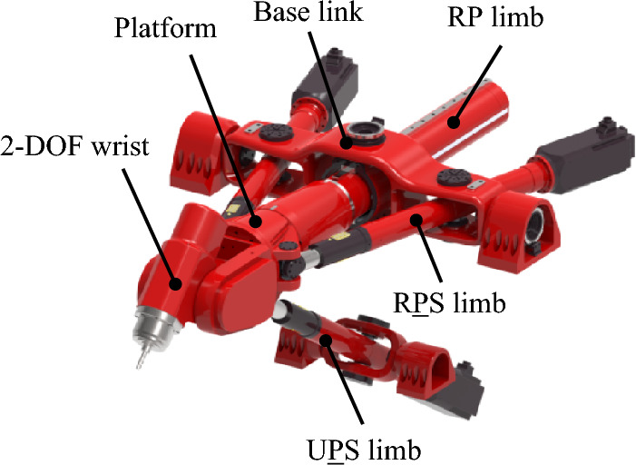
CAD model of the TriMule robot.
Figure 2 shows a schematic diagram of the TriMule robot. For the convenience of description, the UPS limb and two RPS limbs are numbered as limb 1, 2 and 3 respectively. The RP limb plus the A/C wrist is numbered as limb 4, which is composed of five joints and six components numbered 0–5. The five joints include the R joint of the base link, the two joints of the RP limb and the two joints of the A/C wrist, which do not include the spindle. Joint connects the component and . represents the intersection of the two rotating axes of the A/C wrist, and represents the tool tip point.
Figure 2.
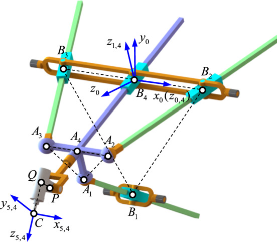
Schematic diagram of the TriMule robot.
In order to effectively describe the position and attitude of each component, the reference coordinate system is established at the point . The axis coincides with the axis of the base link. The axis is perpendicular to the plane determined by . Figures 3 and 4 show the body-fixed frame of the j-th component in the i-th limb and the tool frame established by the D-H method.
Figure 3.
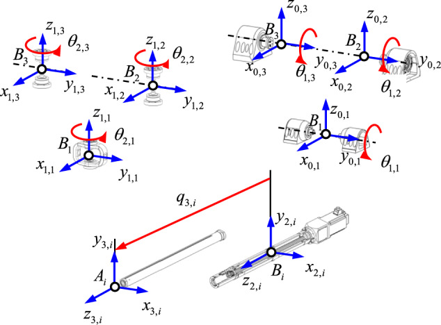
Body-fixed frames of limb .
Figure 4.
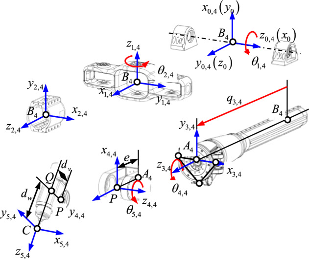
Body-fixed frames of limb 4.
Then the orientation matrix of with respect to can be expressed by
| 1 |
where is the orientation matrix of with respect to , is the orientation matrix of with respect to respectively. Here, , and represent the unit vectors of three coordinate axes of . , and represent that of three coordinate axes of . is the angle of rotation about the axis.
Kinematic analysis
Inverse displacement analysis
The inverse displacement analysis is to solve the two rotation angles of the A/C wrist and the length of three actuated limbs of the parallel mechanism by the known dimensional parameters, tool tip position vector and tool axis vector.
The position vector of P fixed on the platform can be expressed as
| 2 |
| 3 |
where
Here and represent the tool tip vector and the tool orientation vector, is the length of the RP limb, , .
Taking norm on both sides of Eq. (3), leads to
| 4 |
According to Eqs. (2) and (4), the rotation angles and of R(RP) limb can be obtained
| 5 |
Then can be determined. Rewrite Eq. (1) as
| 6 |
Then, the rotation angles and of the A/C wrist can be obtained by
| 7 |
The closed-loop equation formed by limb can be expressed as
| 8 |
where and are the length and unit vector of the actuated limb respectively, .
, , , , .
Taking norm on both sides of Eq. (8), leads to
| 9 |
So far, the inverse displacement solution of the TriMule robot has been solved.
Velocity and acceleration analysis
The velocity analysis is concerned with the determination of axial telescopic velocity () of three actuated limbs of parallel mechanism and angular velocity () of the A/C wrist according to linear velocity vector of tool tip C and tool angular velocity vector .
The velocity vector and can be expressed as
| 10 |
where represents linear velocity vector of point , represents the position vector from point P to point C, , , and represent the C-axis vector and A-axis vector of the wrist, represents the angular velocity vector of the 3-th component in limb 4. Here, the relationship between , () and can be expressed as
| 11 |
where and represent the velocity vector of the actuated joints and the passive joint. , and represent the Jacobian matrices.
Substitute Eq. (11) into Eq. (10), the mapping relationship between joint velocity and operation velocity can be constructed by
| 12 |
where , , is the skew-symmetric matrix of .
The acceleration analysis is concerned with the determination of axial telescopic acceleration () of three actuated limbs of parallel mechanism and angular acceleration () of the A/C wrist according to the acceleration vector of point and tool angular acceleration vector .
Taking the derivatives of Eq. (10) with respect to time yields
| 13 |
where , , is the acceleration vector of point . Here, the relationship between , () and can be expressed as
| 14 |
where .
Substitute Eq. (14) into Eq. (13), we have the acceleration mapping function
| 15 |
where , , , .
Inverse dynamic formulation
The inverse dynamic analysis is concerned with the determination of the driving torque required for achieving a given motion according to the inertia parameters of the moving components, which provides a theoretical basis for analyzing the variation of load inertia of the actuated joints in the whole workspace25,26.
Motion analysis of component centroid
Considering that the mass and inertia of spherical joints, Hooke joints and the connecting frame rotating pair are small, these components are ignored. Therefore, the inertia force and torque in the TriMule robot system are generated by the following components: component 2 (limb outer tube) and component 3 (push rod) in limb (); component 1 (base link), component 2 (outer ring), component 3 (platform assembly), component 4 (C-axis assembly) and component 5 (A-axis assembly and Spindle) in limb 4; the driven assembly of actuated joints (lead screw assembly, A/C wrist driven assembly).
The position vector of the centroid of component in limb can be expressed as
| 16 |
where represents the position vector of centroid measured in , represents the position vector of coordinate origin of measured in .
Taking the first and second derivatives of Eq. (16) with respect to time yields, we can get
| 17 |
where is the Jacobian matrix of component centroid velocity with respect to moving platform velocity.
Inverse dynamic analysis
The virtual work principle can be used to obtain
| 18 |
where and represent the inertia force and torque of each component in limb (), and represent the gravity and gravity torque of each component in limb , () and () represent the inertia torque generated by the actuated joint assembly rotating around its own axis. and represent the external force and torque on the spindle, , () represents the driving torque of the actuated joint in the i-th limb of the parallel mechanism, , () represents the driving torque of the actuated joint in the A/C wrist, is the gear ratio. and () refer to the number of components considering inertia force (torque) or gravity, as shown in Table 1.
Table 1.
The number of components considering inertia force (torque) or gravity.
| 3 | 3 | 2 | 3 | 3 | 3 | 2 | 2 | |
| 3 | 5 | 1 | 5 | 3 | 5 | 0 | 0 |
By rewriting Eq. (18) into matrix form, the dynamic equation of the hybrid robot can be obtained
| 19 |
where represents lead screw pitch, and represent the inertia about their respective axes, respectively, represents the transmission ratio, is identity matrix, and
It can be seen from Eq. (19) that the driving torque of the parallel mechanism consists of two parts: (1) All external force or torque of each component of the whole system; (2) Inertia torque generated by the rotation of the lead screw around its own axis. The driving torque of the A/C wrist consists of two parts: (1) Gravity, inertia torque and external load term of each component; (2) Inertia torque generated by the transmission mechanism of the A/C wrist. It can be seen that has nothing to do with the gravity and inertia force of each component in the parallel mechanism.
Considering that the pose of the wrist and the load inertia around the A/C axis change little in practice7, the variation of the load inertia of each actuated joint of the parallel mechanism is the key issue that needs attention and research. The A/C wrist and the moving platform are regarded as a component, and then the rigid body dynamic equation of the parallel mechanism can be constructed according to Eqs. (16), (17) and Eq. (19) as
| 20 |
where is the inertia matrix of the parallel mechanism in the operating space; is the Coriolis force and centrifugal force acting on the system, which is a function of the position, attitude and velocity of the moving platform; reflects the influence of gravity; refers to the term related to external load. For more information about the mathematical expressions of these components, please refer to26.
The above formula can also be rewritten into the general form of rigid body dynamics equation by considering friction27
| 21 |
where
The inertia matrix of the parallel mechanism in the joint space is only related to the joint position. Let represents the main diagonal element of , then the load inertia can be calculated by . Here, represents the friction force of the i-th actuated joint, , and denote the static, Coulomb, and viscous friction parameters, respectively. It is worth noting that the static and Coulomb friction forces vary with the normal forces, leading to and should be identified accordingly28.
Inertia fast estimation
Analysis of inertia variation and grid estimation method
Due to the load inertia of the actuated joint changes with the configuration of the robot, the calculation of that is significant for motor selection, controller parameter tuning, model-based control method, etc. In this section, a fast estimation method is proposed to quickly and easily calculate the joint inertia of the robot at any configuration in the workspace.
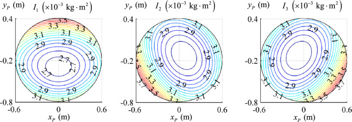
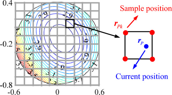
Given the dimensional parameters in29 and the inertial parameters of the main components measured in the body-fixed frames extracted from the CAD model in Table 2, the variation of the joint load inertia in the whole circular workspace is calculated and shown in Fig. 5. Here, 600 × 600 uniformly distributed sample points in the circular workspace are selected, and then the load inertia of each actuated joint at these sample points is calculated by using the dynamic model. Equipped with the inertia information at hand, the contour map can be drawn as shown in Fig. 5. It can be seen from the figure that is distributed in an approximate concentric ellipse from the center to the boundary. The gradient closer to the boundary in the direction of the minor axis of the ellipse is larger, and the fluctuation amount can reach 37%. Here, the circular workspace refers to the 2D workspace of the parallel mechanism, and the 3D workspace of that can be found in reference30. Generally, to solve this kind of fitting problem, firstly divide the workspace into grids as shown in Fig. 6, then determine the sample inertia at the grid nodes through the dynamic model and the corresponding position coordinates, and finally use the inverse distance weighting method to fit the inertia at any configuration:
| 22 |
where represents the estimated value of the load inertia of the i-th actuated joint at the current position , represents the load inertia of the i-th actuated joint at the () sample configuration , . It can be seen from Eq. (22) that this method belongs to a fuzzy algorithm, which estimates inertia by the membership degree of the fuzzy center . However, this method needs to determine the sample inertia at each grid node first, which increases a lot of workload and the burden of calculation and storage.
Table 2.
Inertial parameters of the TriMule robot.
| Limb | Component | (kg) | () | (m) |
|---|---|---|---|---|
| 1, 2, 3 | 1 | 36.02 | ||
| 2 | 13.83 | |||
| 4 | 1 | 115.80 | ||
| 2 | 14.39 | |||
| 4 | 32.03 | |||
| 5 | 38.48 |
Pitch , Inertia of lead screw .
Figure 5.
Contours of inertia in the task workspace.
Figure 6.
Inverse distance weighting method.
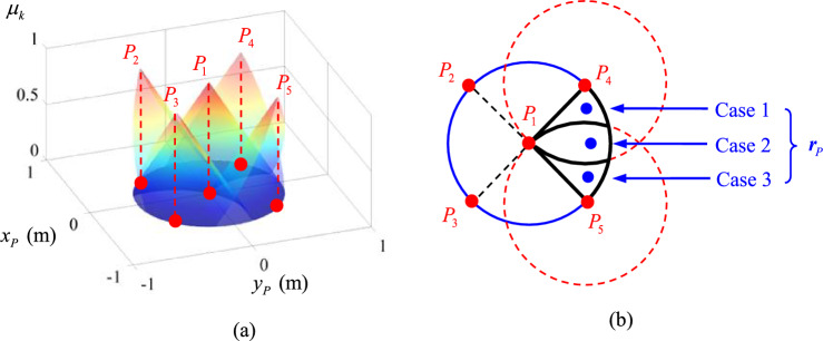
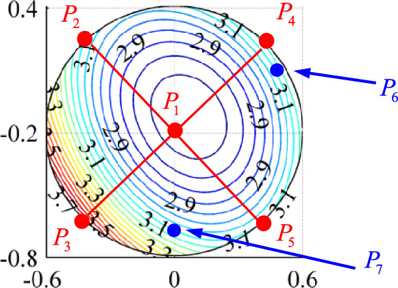
Therefore, it is expected that the global inertia variation can be fitted using only a few sample data. Figure 7a shows the method of using 5 sample points as fuzzy centers to fit the inertia. Then, the inertia at any configuration can be estimated by using the triangle-shape grade of the membership function:
| 23 |
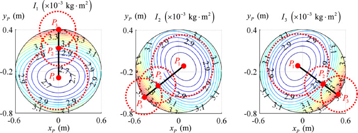
where represents the radius of the workspace, represents the membership degree of the inertia at the current configuration with respect to the inertia at the fuzzy central configuration . Figure 7b shows three general cases of the fuzzy estimation by taking the region as an example. Case 1: the calculation of inertia is only affected by and ; Case 2: the calculation of inertia is affected by , and ; Case 3: the calculation of inertia is only affected by and . It can be seen that this method makes the inertia calculation only depend on the inertia information of the surrounding 2–3 points. In order to verify the effectiveness of this method, the fitting of the inertia of and is analyzed as shown in Fig. 8. In the figure, and are on the same inertia isoline. The calculation of the inertia at is not only affected by the inertia at , but also affected by that at . Obviously, Data at is an interference factor. and are on the same inertia isoline. The calculation of the inertia at is affected by the inertia at , and . Here, data at and are the interference factors. It can be seen that when the number of points as fuzzy centers is small, the estimation of inertia is not accurate if the uniformly distributed fuzzy centers are simply selected. Therefore, the variation of inertia should be further considered when determining the fuzzy center point and constructing the membership function.
Figure 7.
Inertia fitting by fuzzy method.
Figure 8.
Analysis of the proposed method.
Circle membership function fitting
By observing the inertia distribution shown in Fig. 5, it can be seen that the inertia isoline is distributed in the shape of an approximate concentric ellipse, so it is advisable to select the fuzzy center in the direction of the minor axis of the ellipse, and then choose the triangular membership function for fitting, as shown in Fig. 9. In the figure, , , represent the points on the isoline corresponding to the minimum value, global mean value and maximum value of inertia, respectively. Let be fixed, moves on the circle with as the center and as the radius, and moves on the circle with as the center and as the radius, then the influence range of these points can cover the whole circular workspace. Accordingly, the algorithm of Eq. (23) is improved as follows:
| 24 |
where
Figure 9.
Improved fuzzy fitting method.
Here , , represent the position vectors of , , in frame .
According to Eq. (24), the circle membership function (CMF) covering the whole workspace can be drawn, as shown in Fig. 10. Employed by the membership function and the inertia information shown in Table 3, the variation of the load inertia of each actuated joint in the whole workspace is fitted, as shown in Fig. 11. It can be seen from the figure that the fitting results are similar to the theoretical results shown in Fig. 5. However, since the membership function is constructed by scanning the entire workspace along the circular track using the triangular membership function, the fitted isoline is still quite different from the approximate elliptical isoline in Fig. 5.
Figure 10.
Circle membership function.
Table 3.
Configuration information for constructing circle membership function.
| Minimum value () | Global mean value () | Maximum value () | ||||
|---|---|---|---|---|---|---|
| Inertia | Inertia | Inertia | ||||
| Joint1 | 2.65 | 2.83 | 3.51 | |||
| Joint2 | 2.69 | 2.88 | 3.69 | |||
| Joint3 | 2.69 | 2.88 | 3.69 | |||
Inertia (), (m)
Figure 11.
Fitting results of circle membership function.
Ellipse membership function fitting
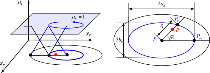
The membership function is constructed by scanning the entire workspace along the elliptical track instead of the circular track, as shown in Fig. 12. In the figure, and represent the length of the long semi axis and the short semi axis of the ellipse, respectively. Then the ellipse membership function (EMF) can be constructed by
| 25 |
where
Figure 12.
Ellipse membership function.
Here represents the parameter angle of the elliptic parametric equation, and represent the position vectors of the ellipse center point and the major axis vertex , respectively. Accordingly, given the parameters shown in Table 4, the membership function covering the whole workspace is drawn, as shown in Fig. 13. The variation of the load inertia of each actuated joint in the whole workspace is fitted as shown in Fig. 14. It can be seen from the figure that the fitting results are very close to the theoretical results shown in Fig. 5.
Table 4.
Configuration information for constructing ellipse membership function (m).
| , | , | , | |||
|---|---|---|---|---|---|
| Joint 1 | 0.11, 0.09 | 0.52, 0.35 | 0.78, 0.69 | ||
| Joint 2 | 0.12, 0.08 | 0.56, 0.35 | 0.87, 0.82 | ||
| Joint 3 | 0.12, 0.08 | 0.56, 0.35 | 0.87, 0.82 |
Figure 13.
Ellipse membership function.
Figure 14.
Fitting results of ellipse membership function.
Verification
Simulations
In this section, simulations will be carried out to verify the effectiveness of the proposed methods. The simulations are designed to examine two important issues: (1) the accuracy of calculating inertia; (2) the simplicity and fastness of the algorithms.
Figures 15 and 16 show the errors of the fitting results of Figs. 11 and 14 relative to the theoretical results of Fig. 5 respectively. The maximum values and global mean values of the errors are shown in Table 5. It can be seen that the maximum values and the global mean values of the fitting errors of the elliptic membership function are within and respectively. Compared with the fitting errors of the circle membership function, the maximum value and the global mean value of the fitting errors of joint 1 are reduced by 39.18% and 65.79%, and those of joint 2 and 3 are reduced by 51.23% and 81.25%, which proves that the ellipse membership function has better global fitting accuracy.
Figure 15.
Fitting errors of circle membership function.
Figure 16.
Fitting errors of ellipse membership function.
Table 5.
Fitting errors of two membership functions ().
| Errors of Joint 1 | Errors of Joint 2 | Errors of Joint 3 | ||||
|---|---|---|---|---|---|---|
| Maximum value | Global mean value | Maximum value | Global mean value | Maximum value | Global mean value | |
| CMF | 0.268 | 0.076 | 0.447 | 0.128 | 0.447 | 0.128 |
| EMF | 0.163 | 0.026 | 0.218 | 0.024 | 0.218 | 0.024 |
| Percent reduction | 39.18% | 65.79% | 51.23% | 81.25% | 51.23% | 81.25% |
Table 6 shows the memory space occupied and computation time of the three algorithms: the dynamic model-based estimating algorithm, the grid estimating algorithm, and the fuzzy estimating algorithm with the ellipse membership function. It can be seen from the table that the memory space of the grid estimating algorithm is much larger than that of other algorithms. Here, the inertia values of 900 × 900 grid nodes occupy 10,421.06 kb and the inverse distance weighting calculation occupies only 1.41 kb, leading to a large amount of offline identification work and fewer online computing burden. The fuzzy estimating algorithm with the ellipse membership function occupies the minimum memory space, which can perform one operation within 4 ms less than the trajectory interpolation period of 10 ms.
Table 6.
The memory space occupied and computation time of the three estimating algorithms.
| The dynamic model-based estimating algorithm | The grid estimating algorithm | The fuzzy estimating algorithm with ellipse membership function | |
|---|---|---|---|
| The memory space (kb) | 8.26 | 10,422.47 | 3.18 |
| The computation time (ms) | 50.01 | 2.75 | 3.06 |
Experiments
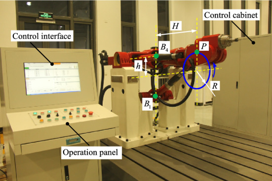
In this section, the proposed method for inertia fast estimation will be verified by experiments. Figure 17 shows the realized prototype of the TriMule robot and the verifying path. Equipped with an IPC + Turbo PMAC-PCI CNC system, the robot can move the platform reference point P at a maximum speed and acceleration of 60 m/min and 10 m/s2, respectively.
Figure 17.
The prototype of the TriMule robot and the verifying path.
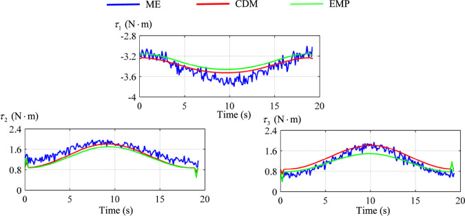
To verify the effectiveness of the new estimation algorithm, the circular path was planned with R = 0.3 m, H = 1.2 m, h = 0.19 m by taking the values of 30 m/min and 5 m/s2 for the maximum velocity and acceleration of P along the path. The driving torque of each actuated joint is measured from the servo driver by employing the data acquisition card and Labview program. Figure 18 shows the driving torque of each actuated joint with time obtained by measurement experiments (ME), calculation using the dynamics model (CDM) and estimation using the proposed method (EPM). Here, the inertial torques are computed by CDM or EPM and the other torque components are computed by using the same dynamic model. It can be seen that three torque curves are similar and the root mean squares (RMS) of errors with CDM or EPM relative to ME listed in Table 7 are within . These deviations are caused by the fitting errors of the elliptical membership function as shown in Fig. 16, which is within an acceptable range. As compensation, the proposed method has a lower computational complexity compared to using the dynamic model, leading to the reduction of the computational memory burden.
Figure 18.
The driving torque of each actuated joint with time.
Table 7.
The RMS of joint torque errors along the verifying path.
| Joint 1 | Joint 2 | Joint 3 | |
|---|---|---|---|
| CDM | 0.27 | 0.64 | 0.50 |
| EPM | 0.32 | 0.66 | 0.57 |
Conclusions
This paper presents the dynamic formulation and a method for inertia fast estimation of a hybrid robot. The conclusions are drawn as follows.
Based on the analysis of kinematics and rigid body dynamics, the distribution of the load inertia of each actuated joint of the parallel mechanism in the whole workspace is revealed, and the isolines of that are approximately concentric ellipses.
The method for fitting the inertia distribution, which only uses the inertia information of a few configurations, is proposed using the circle or elliptical membership function. The results show that the elliptical membership function has better global fitting accuracy in comparison with the circle membership function and the torque estimation accuracy is within an acceptable range.
The proposed method is also applicable to the off-diagonal elements of the inertia matrix (joint couplings) and the joint load inertia of other parallel mechanisms. It can be used to quickly predict other control variables (PID parameters and acceleration feedforward parameters) affected by the inertia, allowing the algorithm to be easily integrated into the robot control system.
Acknowledgements
This work was supported by the Natural Science Foundation of Tianjin (23JCQNJC00430), the National Natural Science Foundation of China (NSFC) (Grant 52205029, 52205030, 52375026), State Key Laboratory of Robotics and Systems (HIT) (SKLRS-2023-KF-07). The authors sincerely thank Professor Huang at Tianjin University for the help in dynamic modeling. The authors also thank the editors and reviewers for their patient work and constructive suggestions.
Author contributions
Q.L.: Conceptualization, Methodology, Software, Writing- original draft. T.Y.: Validation, Writing- review & editing. B.L.:Validation, Writing -review & editing. Y.M.: Supervision, Writing-
Data availability
Due to [reasons for data non disclosure], the datasets generated and/or analyzed during the current research period are not publicly available, but can be obtained from the corresponding author.
Competing interests
The authors declare no competing interests.
Footnotes
Publisher's note
Springer Nature remains neutral with regard to jurisdictional claims in published maps and institutional affiliations.
References
- 1.Bi, Z. & Jin, Y. Kinematic modeling of parallel kinematic machine exechon. Robot. Comput.-Integr. Manuf.27(1), 186–193 (2011). 10.1016/j.rcim.2010.07.006 [DOI] [Google Scholar]
- 2.Neumann, K. E., Tricept application. In Proceedings of the 3rd Chemnitz Parallel Kinematics Seminar (2002).
- 3.Neumann, K. E., The key to aerospace automation. In Proceedings of the SAE Aerospace Manufacturing and Automated Fastening Conference and Exhibition (2006).
- 4.Yao, J. et al. Dynamic analysis and driving force optimization of a 5-DOF parallel manipulator with redundant actuation. Robot. Comput.-Integr. Manuf.48, 51–58 (2017). 10.1016/j.rcim.2017.02.006 [DOI] [Google Scholar]
- 5.Huang, T. et al. A method for estimating servomotor parameters of a parallel robot for rapid pick-and-place operations. ASME J. Mech. Des.127(4), 596–601 (2005). 10.1115/1.1898343 [DOI] [Google Scholar]
- 6.Choi, H., Company, O. & Pierrot, F, et al. Design and control of a novel 4-DOFs parallel robot H4. In Proceedings of IEEE International Conference on Robotics and Automation, Taipei, Taiwan pp. 1185–1191 (2003).
- 7.Liu, Q. et al. An iterative tuning approach for feedforward control of parallel manipulators by considering joint couplings. Mech. Mach. Theory140, 159–169 (2019). 10.1016/j.mechmachtheory.2019.05.017 [DOI] [Google Scholar]
- 8.Ogbobe, P., Jang, H. & He, J., et al. Analysis of coupling effects on hydraulic controlled 6 degrees of freedom parallel manipulato rusing joint space inverse mass matrix. In The Second International Conferences on Intelligent Computation Technology and Automation, Changsha, China, pp. 845–858 (2009).
- 9.Li, M. et al. Dynamic formulation and performance comparison of the 3-DOF modules of two reconfigurable PKM—the Tricept and the TriVariant. J. Mech. Des.127(6), 1129–1136 (2005). 10.1115/1.1992511 [DOI] [Google Scholar]
- 10.Shao, Z., Tang, X., Chen, X. & Wang, L. Research on the inertia matching of the Stewart parallel manipulator. Robot. Comput.-Integr. Manuf.28, 649–659 (2012). 10.1016/j.rcim.2012.04.001 [DOI] [Google Scholar]
- 11.Mo, J. et al. Dynamic performance analysis of the X4 high-speed pick-and-place parallel robot. Robot. Comput.-Integr. Manuf.46, 48–57 (2017). 10.1016/j.rcim.2016.11.003 [DOI] [Google Scholar]
- 12.Codourey, A. Dynamic modeling and mass matrix evaluation of the Delta parallel robot for axes decoupling control. In Proceedings of the 1996 IEEE/RSJ International Conference on Intelligent Robots and Systems, Osaka, Japan, pp. 1211–1218 (1996).
- 13.Shao, Z. et al. Inertia match of a 3-RRR reconfigurable planar parallel manipulator. Chin. J. Mech. Eng.22(6), 791–799 (2009). 10.3901/CJME.2009.06.791 [DOI] [Google Scholar]
- 14.Luo, Z. et al. A dynamic parameter identification method for the 5-DOF hybrid robot based on sensitivity analysis. Ind. Robot- Int. J. Robot. Res. Appl.51(2), 340–357 (2024). 10.1108/IR-08-2023-0178 [DOI] [Google Scholar]
- 15.Briot, S. & Gautier, M. Global identification of joint drive gains and dynamic parameters of robots. J. Dyn. Syst. Meas. Control-Trans. ASME33, 3–26 (2015). [Google Scholar]
- 16.Corigliano, A. & Mariani, S. Parameter identification in explicit structural dynamics: Performance of the extended Kalman filter. Comput. Methods Appl. Mech. Eng.193(36–38), 3807–3835 (2004). 10.1016/j.cma.2004.02.003 [DOI] [Google Scholar]
- 17.Ding, J. et al. Particle filtering based parameter estimation for systems with output-error type model structures. J. Frankl. Inst.-Eng. Appl. Math.356(10), 5521–5540 (2019). 10.1016/j.jfranklin.2019.04.027 [DOI] [Google Scholar]
- 18.Urrea, C. & Pascal, J. Design and validation of a dynamic parameter identification model for industrial manipulator robots. Arch. Appl. Mech.91(5), 1981–2007 (2021). 10.1007/s00419-020-01865-2 [DOI] [Google Scholar]
- 19.Taie, W., ElGeneidy, K. & AL-Yacoub, A. Online identification of payload inertial parameters using ensemble learning for collaborative robots. IEEE Robot. Autom. Lett.9(2), 1350–1356 (2024). 10.1109/LRA.2023.3346268 [DOI] [Google Scholar]
- 20.Wang, X., Liu, B. & Mei, X. Genetic algorithm for dynamic parameters estimation of the machine tool worktable using the residual vibration signal. J. Vib. Control28(11–12), 1433–1440 (2022). 10.1177/1077546321993579 [DOI] [Google Scholar]
- 21.Li, H., Jiang, J. & Mohamed, M. Online dynamic load identification based on extended kalman filter for structures with varying parameters. Symmetry-Basel13(8), 1372 (2021). 10.3390/sym13081372 [DOI] [Google Scholar]
- 22.Tang, J. et al. Parameter identification of inverter-fed induction motors: A review. Energies11(9), 2194 (2018). 10.3390/en11092194 [DOI] [Google Scholar]
- 23.Chen, C., Zhang, W. & Liu, T. Online identification of inertial parameters of a robot with partially combined links using IMU sensing. Mechatronics94, 103023 (2023). 10.1016/j.mechatronics.2023.103023 [DOI] [Google Scholar]
- 24.Hametner, C. & Jakubek, S. Local model network identification for online engine modelling. Inf. Sci.220, 210–225 (2013). 10.1016/j.ins.2011.12.034 [DOI] [Google Scholar]
- 25.Zhao, Y., Mei, J., Niu, W., Wu, M. & Zhang, F. Coupling analysis of a 5-degree-of-freedom hybrid manipulator based on a global index. Sci. Prog.103(1), 1–21 (2020). 10.1177/0036850419881896 [DOI] [PMC free article] [PubMed] [Google Scholar]
- 26.Dong, C., Liu, H., Xiao, J. & Huang, T. Dynamic modeling and design of a 5-DOF hybrid robot for machining. Mech. Mach. Theory165, 104438 (2021). 10.1016/j.mechmachtheory.2021.104438 [DOI] [Google Scholar]
- 27.Yang, X. et al. Continuous friction feedforward sliding mode controller for a Trimule hybrid robot. IEEE/ASME Trans. Mechatron.23(4), 1673–1683 (2018). 10.1109/TMECH.2018.2853764 [DOI] [Google Scholar]
- 28.Rosyid, A. & El-Khasawneh, B. Identification of the dynamic parameters of a parallel kinematics mechanism with prismatic joints by considering varying friction. Appl. Sci.10(14), 4820 (2020). 10.3390/app10144820 [DOI] [Google Scholar]
- 29.Liu, Q. & Huang, T. Inverse kinematics of a 5-axis hybrid robot with non-singular tool path generation. Robot. Comput.-Integr. Manuf.56, 140–148 (2019). 10.1016/j.rcim.2018.06.003 [DOI] [Google Scholar]
- 30.Dong, C., Liu, H., Yue, W. & Huang, T. Stiffness modeling and analysis of a novel 5-DOF hybrid robot. Mech. Mach. Theory125, 80–93 (2018). 10.1016/j.mechmachtheory.2017.12.009 [DOI] [Google Scholar]
Associated Data
This section collects any data citations, data availability statements, or supplementary materials included in this article.
Data Availability Statement
Due to [reasons for data non disclosure], the datasets generated and/or analyzed during the current research period are not publicly available, but can be obtained from the corresponding author.


