On formal limitations of causal ecological networks

Abstract

Causal multivariate time-series analysis, combined with network theory, provide a powerful tool for studying complex ecological interactions. However, these methods have limitations often underestimated when used in graphical modelling of ecological systems. In this opinion article, I examine the relationship between formal logic methods used to describe causal networks and their inherent statistical and epistemological limitations. I argue that while these methods offer valuable insights, they are restricted by axiomatic assumptions, statistical constraints and the incompleteness of our knowledge. To prove that, I first consider causal networks as formal systems, define causality and formalize their axioms in terms of modal logic and use ecological counterexamples to question the axioms. I also highlight the statistical limitations when using multivariate time-series analysis and Granger causality to develop ecological networks, including the potential for spurious correlations among other data characteristics. Finally, I draw upon Gödel’s incompleteness theorems to highlight the inherent limits of fully understanding complex networks as formal systems and conclude that causal ecological networks are subject to initial rules and data characteristics and, as any formal system, will never fully capture the intricate complexities of the systems they represent.

This article is part of the theme issue ‘Connected interactions: enriching food web research by spatial and social interactions’.

1. Causal networks in ecology: insides or illusions?

Ecological networks are graphical model representations of biotic interactions and their physical environment, serving as valuable tools for studying the structure, function and stability of real ecosystems [1]. Unlike other networks involving objects, individuals or other entities, ecological networks are typically composed of organisms, populations and communities that engage in trophic, predator–prey, mutualistic and competitive relationships [2]. Moreover, in contrast to static networks, ecological networks are dynamic systems that continuously evolve in response to environmental changes, disturbances and evolutionary processes [3]. The application of ecological networks in ecological research can be traced back to the late 1970s when Robert May introduced the concept of food webs, which represent trophic interactions between species in an ecosystem [4]. Since then, the study of ecological networks has evolved and expanded to include other types of ecological interactions [5–7].

Ecological networks (i.e. ecological webs) typically focus on static interactions and relationships between species or ecological entities, often relying on a priori definitions or statistical correlations [8]. On the other hand, time-series networks are an extension of traditional networks that incorporate temporal dynamics by considering changes and interactions over time, as well as the uncertainty and variability that are inherent in the systems [9,10]. By incorporating time-series data into network models, researchers can explore the causal links between ecological variables, as for instance species abundances and environmental factors [11], distribution-abundance relationships [12], ecology of parasite transmission [13] and the functioning of complex ecosystem processes [14,15].

Conceptually, they consist of graphical representations that aim to capture the causal relationships among ecological variables in a dynamic system [16,17]. These networks are constructed using statistical connectivity measures, such as Granger causality or other causality indexes (e.g. transfer entropy, directed information, etc.), to infer the presence and direction of causal interactions between variables [18]. In such a multivariate network, each variable is represented as a node, and statistically significant relationships between variables are represented as directed edges connecting the nodes [17].

In the development of networks, two main factors play a role. The first is the philosophical–logical background with which causality is defined. These are the rules that form the axioms for the derivation of true causality. The second is related to inherent data properties and statistics. It is evident that using various rules and statistical measures can result in different network configurations leading to questionable conclusions [7,17,19]. To date, Granger, who proposed the Granger causality test, which was awarded the Nobel Prize in 2003, has stressed that some studies using ‘Granger causality’ testing in areas outside of economics have reached ‘ridiculous’ conclusions [20,21]. Additionally, ecological networks consist of rule-based graph-theoretic objects, and as such, are subject to Gödel’s incompleteness theorems, which state that no consistent axiomatic system can prove all truths [22,23].

As a result, an essential question arises: are ecological networks reliable and unbiased logical representations of true causal flows within complex systems? Or are they simply products of the researcher’s compromise with simplified products of axiomatic norms, statistical assumptions and intuitive knowledge?

In this context, the aim of this opinion article is to explore the limitations of ecological networks as a formal system in detecting true causation within multivariate complex ecological systems. We consider ecological networks as formal systems and are concerned with approaching causality rules through modal logic statements (i.e. propositions) that can be either true or false, but not both. This provides us with a tool to show through counterexamples that in many ecological networks the causality rules might be violated. In addition to logical paradoxes, we aim to outline the statistical limitations of Granger causality and, finally, to bring into consideration the inherent incompleteness of ecological networks as true representations of the system under consideration. Our purpose is not to examine every mathematical aspect of ecological networks and causality definitions, as this is virtually impossible. Instead, we want to draw attention to the basic drawbacks of causal networks, whether they be logical, statistical or formal. By doing this, we intend to promote a more cautious approach to interpreting ecological networks and reaching scientific conclusions.

2. Discrepancies between ecological evidence and logical reasoning

The scientific exploration of causal ecological interactions, while not new, has consistently grappled with the challenge of accurately modelling the dynamic interplay and feedback mechanisms within ecosystems. Despite the advancements in understanding density dependence, ecological interactions and population stability, network models often fall short of capturing the true complexity of these systems [24]. This is particularly evident in even ‘simple’ interactions such as those between predators and prey, where observed patterns are influenced by direct responses to environmental changes, self-regulation mechanisms and the presence of competing predators. Such complexity underscores the limitations of relying solely on common-sense intuitions, as noted by Levins & Schultz [25], who highlight the often-misleading nature of intuitive arguments in understanding ecological dynamics.

Additionally, seminal works, including those by Levins & Puccia [26], have long demonstrated that ecological interactions are far from simple to describe and have made significant contributions to the understanding of multitrophic interactions. However, although research has highlighted that the simplification of interaction networks, which do not account for dynamic changes in intra and interspecies interactions, can lead to incorrect conclusions and oversimplifications [25,26], it is still challenging to explicitly formalize and prove causal links through mathematical induction and reasoning. Even though these studies are very helpful, they show that many attempts are still not successful in understanding the underlying causal mechanisms. This emphasizes the necessity for a more thorough application of logic and mathematical concepts to comprehend the limits of causal ecological networks.

Using logic to ascertain causality is not new, but its application in ecological networks is a significant leap forward in holistically addressing the challenges in identifying causal links within ecological systems. To name a few seminal works, Halpern & Pearl [27] provide logic-based definitions of actual causes where logical formulas with events formalize counterfactuals. Judea Pearl, particularly, has significantly influenced the field of causal modelling, including its application in ecology and emphasized the importance of explicitly representing causal assumptions in ecological models, moving beyond simple correlations. The structural equation models (SEMs), for instance, capture the logical and causal interactions among ecosystem variables, using directed acyclic graphs to map hypothesized relationships [28]. Yet, SEMs require well-defined a priori hypotheses about these interactions, assuming deep knowledge of the system’s causal structure.

Rubin’s causal model [29] and Pearl’s do-calculus [30], provide structured frameworks for causal inference, including elements of formal logic; their application to ecological networks is challenged by the complexity of these systems, data limitations and the need for explicit, sometimes untestable assumptions. Another advanced and powerful approach for constructing causal ecological networks is the use of Bayesian models [31], yet they do not inherently involve logical causal reasoning while the choice of priors can be subjective and controversial, especially in the absence of clear prior knowledge. To bridge such gaps, emerging approaches as those proposed by Barbero et al. [32], seek to redefine the basis of causal inference into general epistemic reasoning. More recently, modal logic has also been proposed and applied as a formal language for describing and explaining correctness in statistical causality in life science trials by incorporating modal operators for interventions to express causal properties between probability distributions in different possible worlds in a Kripke model [33].

In this context, by leveraging modal logic, we shift the analysis from strictly ecological to mathematical perspectives, enabling the validation of ecological causality with an understanding of axiomatic limitations. This approach complements existing research and, despite potential limitations, frames ecological network challenges within broader epistemological constraints and their implications for knowledge discovery.

3. Causality in symbolic logic: challenges in complex ecological systems

Causality is a central topic in both epistemological inquiry and practical application in sciences. Here I present a short account of causality, formalize causal rules using modal logic and highlight potential paradoxes when implemented in the context of ecological networks. The formal definitions of key symbols and operators in modal logic that will be used, along with their semantic contexts for causal inference, are briefly described in table 1.

Table 1.

Formal definitions and semantic context of key symbols and operators in modal logic for causal inference.

symbol/operator	definition	semantics and usage in causal logic
A, B, C,… P, Q, R,… X, Y, Z,…	propositional variables	commonly used uppercase letters to denote specific propositions, statements or variables
W1, W2, W3	possible worlds: a world that could have been, but is not	each possible world corresponds to a unique set of possible causal relationships and events, between variables evaluated, allowing us to explore the counterfactual implications of different causal structures
∧	conjunction: and	represents a logical ‘and’ operator in causal logic
∨	disjunction: or	represents a logical ‘or’ operator in causal logic
${\displaystyle \mathrm{\neg }}$	negation: not	denotes the absence or negation of an event or condition
${\displaystyle \to }$	logical Implication: if …, then …	consequence/causality between variables
${\displaystyle \leftrightarrow }$	logical biconditional (if and only if)	bidirectional or mutual causality between variables
${\displaystyle \diamond }$	possibility: is possible	the proposition is possibly true if there exists at least one possible world in which it is true
${\displaystyle ◻}$	necessity: is necessary	the proposition is necessary if it is true in all possible worlds
d	distance between possible worlds: the number of changes that are needed to convert one possible world into another	d(W1, W2) represents the number of changes that are needed to convert possible world W1 (network configuration 1) into possible world W2 (network configuration 2)

I will start with David Lewis’s influential definition of causality based on counterfactual dependence [34]. The framework is guided by three axioms [35]: axiom 1: ‘If A were the case, C would be the case is true in the actual world if and only if (i) there are no possible A-worlds, or (ii) some A-world where C holds is closer to the actual world than is any A-world where C does not hold’. Axiom 2: ‘The set of possible worlds is a complete and consistent set’. Axiom 3: ‘The distance function d(w) is a metric on the set of possible worlds’. The symbols A and C are used here for direct comparison with the initial definitions of counterfactual causality; they do not imply any abbreviation and just serve as placeholders for specific statements or conditions relevant to a causal relationship. The same applies subsequently to the use of other uppercase letters in modal logic (table 1). To formalize causal networks, it is convenient to describe the axioms using modal logic [36], which provides a compact and concise language to formalize causality as follows:

Axiom 1: (□¬𝐴∨□𝐶)∧(∀w:□ →𝐶)→d(w)<d(𝑤′)) (1)

where $◻$ is the modal operator representing necessity, ¬, negation, ∧, conjunction, w, the set of possible worlds and $\mathrm{d}$ , the distance function measuring closeness between the possible worlds [37,38].

Axiom 2: (∀w: P(w) ∨ ¬P(w)) ∧ □(∀w: ¬(P(w) ∧ ¬P(w))) (2).

This can be translated as for every possible world (w), P holds in that world (P(w)), or, not-P holds in that world (¬P(w)), and, it is necessarily true that for every possible world (w), it is not possible that both, P to hold and not-P to hold in that world (¬(P(w) ∧ ¬P(w))).

Axiom 3: ∀w1, w2, w3, … : d(w1) ≥ 0 ∧ d(w1) = 0 ↔ w1 = w2 ∧ d(w1) + d(w2) ≥ d(w3) (3).

This expression asserts that for any possible worlds w1, w2, w3 and so on, the distance function d(w) is non-negative (d(w1) ≥ 0), and the distance function is equal to zero if and only if w1 is equal to w2 (d(w1) = 0 ↔ w1 = w2), and the sum of the distances between w1 and w2 is greater than or equal to the distance between w1 and w3 (d(w1) + d(w2) ≥ d(w3)).

Using the conjunction operator, we can combine the three axioms into a single modal logic statement:

(□((¬A ∨ C) ∧ (∀w: (A → C) → (d(w) < d(w')))) ∧ (∀w: (P(w) ∨ ¬P(w))) ∧ □(∀w: ¬(P(w) ∧ ¬P(w))) ∧ (∀w1, w2, w3,…: d(w1) ≥ 0 ∧ (d(w1) = 0 ↔ w1 = w2) ∧ (d(w1) + d(w2) ≥ d(w3)))) (4).

These statements provide a formal framework for causality reasoning, but the interpretation of possible words depends on the context and requires definition. In ecological networks, we connect possible worlds to alternative network configurations based on varying conditions, interactions and causal influences [39,40]. Thus, possible worlds do not represent all possible network outcomes in the probabilistic sense, but rather capture the various counterfactual scenarios in which causal relationships could have played out, thus serving here a different purpose from that of probability theory.

An inherent key challenge for the counterfactual definition of causality is the problem of implausible cases (PIC). The problem arises when we try to compare different possible cases or worlds to establish causal relationships [41]. In the PIC problem, we can encounter the following ecological counterexample. Let us consider four possible worlds: World 1: A pollutant is released (A is true), and the fish population dies (C is true). World 2: The pollutant is not released (A is false), and the fish population does not die (C is false). World 3: The pollutant is released (A is true), and the fish population does not die (C is false). World 4: The pollutant is not released (A is false), and the fish population dies (C is true). In this example, worlds 1 and 2 are both possible but worlds 3 and 4 are unlikely to occur. Since there exists at least one possible world (w) where the combination of A and C is implausible, the PIC problem can be expressed as follows: □(A → C) ∧ ∃w : ¬(A ∧ C).

Pearl extended Lewis’s causality with structural causal models (SCM), using a directed acyclic graph (DAG) to represent causality [42]. To draw a causal relationship, between a cause variable A and the effect variable C, the following conditions or axioms need to be satisfied: (i) a statistical association between A and C, (ii) a temporal order, with A preceding C, and (iii), the absence of unmeasured or uncontrolled variables (confounders) that can explain the observed association [42].

We formalize Pearl’s causality rules using logic as follows:

Axiom 1: ◇(A ∧ C) or equivalently ◇(A → C) (5).

This represents that there is a possibility of both A and C being true based on a statistical test. It can also be formalized as: (A ∧ C) → ◇(A → C).

Axiom 2: □(A → □C) (6).

This indicates that if A is true then it follows that C must also always (e.g. necessary) be true.

Axiom 3: ¬(∃Z)(Z ∧ (A → C)) (7).

This eliminates any unmeasured confounders by ruling out any variable Z with a causal relationship between A and C.

Combining all three conditions we get:

□(A → □C) ∧ ◇(A → C) ∧ ¬(∃Z)(Z ∧ (A → C)) (8).

Statement (8) establishes causality when all three conditions of statistical association, temporal order and absence of confounders are met.

These formal definitions of causality through logical rules are often intuitively implemented to develop and infer causal networks. However, its validity in detecting ecological interactions depends on satisfying the axioms. I will try to provide some ecological examples that challenge this assumption (table 2).

Table 2.

Summary of causality axioms, ecological counterexamples, corresponding modal propositions and the interaction network for each case (details in text).

axiom and logical expression	counterexample	problem and logical expression	interaction network a
Lewis 1: ‘counterfactual rule over possible worlds’, (◻¬𝐴 ∨ ◻𝐶) ∧ (∀w:◻(A→𝐶)→d(w) < d(𝑤′))	pollutant(s) (A) – fish(es) (C)	‘implausible world cases’: ◻(A → C) ∧ ∃w : ¬(A ∧ C) (whenever A is true, C must also be true in every possible world (i.e. in all combinations of A and C) and there exists at least one possible world (w) where the combination of A and C is implausible, and thus counterfactual dependency cannot be tested)
Pearl 1: ‘statistical association between A and C’,(A ∧ C) → ◇(A → C)	rain (A) – malaria (C), environment (Z)	‘correlation does not imply causation’:◇(A ∧ C) ∧ ◻ (¬ (A → C)) (there exists at least one possible scenario where A and C are correlated, but there is no strict causal relationship between A and C in all possible worlds)
Pearl 2: ‘temporal order, with A preceding C’, □(A → □C)	species learning escape (A), reproduce more (R), evolved genetic trait of species to escape (C)	‘time-reversal causality scenario’: ◇A → R ∧ R → □C ∧ ◇C → □A (the possibility of a behaviour (A), increase is possibility of reproduction (R), and precedes the necessity of the population’s genetic adaptation (C), to establishing the behaviour as necessary)
Pearl 3: ‘absence of any confounders Z’, ¬(∃Z)(Z ∧ (A → C))	fish exposed in pollutant (A), fish exposed in parasite (B), fish dyes (C), confounding variable (Z)	‘common cause’: (A → C) ∧ (B → C) ∧ ¬(∃Z)(Z ∧ (A → C) ∧ (B → C)) (there are causal relationships between A and C, and B and C, and there are no Z influencing these causal relationships)
Granger 1: ‘past and present may cause future, not the opposite’, □(A → C) ∧ □ (¬ (A → C))	predator(s) (A) – prey(s) (C), pollinator(s) (A) – plant(s) (C)	‘cyclical and bidirectional causal flows’, ‘mutual interactions’, □(A → C) ∧ □(C → A) (the necessity of a vice versa causal loop between P and Q)
Granger 2: ‘exclusion of redundant variables’: □(¬(Zn → Ώn))	pollinators (X,Y) and plants (A,B)	‘redundancy problem’: □((A ∧ B) → ◇(¬(Zn → Ώn)) (there exists at least one possible world where Zn does not imply redundant information in the set of all knowledge Ώn)
Granger 3: ‘time continuity’ □(P → Q), $\forall t_i$ , i = 1,2..	Wolbachia (W) – mosquito (M) – disease resistance (R) and environment (E) interactions	‘time-varying interactions’: ◇(M → W) ∧ □(W → R) ∧ □(E → M → R) ∧ □(M → W)) (there exists at least one possible world where (M) affects (W), and in that world, it is necessarily true (□) that (W) causes (R). However, in all possible worlds, changes in (E) cause chain variations in (M) and (R), which, in turn, can affect W)

^a Dashed arrows represent questionable causal connections that cannot be directly tested due to the counterfactual nature of the system under consideration.

Axiom 1 (statement 5) has two challenges: correlation without time lag does not imply causation [17,42] and statistical inference relies on accurate data assumptions [43]. The first is a well-known fallacy and thus we will give just a short example and not delve deeper. The false conclusion that rainfall causes malaria because they are simply correlated, ignores the causal relationship between rainfall and an increase in the mosquito population, which in turn increases the incidence of malaria. The second challenge will be outlined in §4.

Axiom 2, statement (6), is related to the problem of time order (PTO). However, it is well proven that ecological systems have complex dynamics, characterized by mutualistic interactions, feedbacks, loops and chain events and thus it is not always possible to determine the precise order of events [44,45]. One quite interesting example, in which cause and effect may not strictly follow a linear temporal order, is the Baldwin effect [46,47]. We consider the mind example of a bird species that lives in an environment with predators. The individuals that can escape from predators are more likely to survive, reproduce (R) and thus evolve to have a trait of improved escaping (A). This behaviour in turn puts pressure on the population to evolve even better (C). Thus, the evolution of the trait through the possibility of learning (A) precedes the population’s genetic necessity of adaptation (C), or: ◇A → R ∧ R → □C ∧ ◇C → □A. This conclusion challenges the time order in causality since it suggests that individual behaviour through learning and acquired traits, might influence the evolutionary pathways of a population even when learning occurs before the genetic changes. It is clear that we recognize a logical paradox, not a temporal one in the narrow sense.

Another critique of counterfactual causality implemented in ecological systems is the problem of common cause (PCC), which challenges axiom 3 and arises when a variable influences both the cause and the effect [17]. Another ecological example helps illustrate this issue. Consider a population of fish exposed to both a pollutant and a parasite, both of which independently cause the fish to die. In this case, the pollutant and the parasite act as common causes of the fish dying. It becomes challenging to determine whether the pollutant, the parasite or both are responsible for the fish’s death. In this example, the presence of the common cause variable Z violates the non-confounding condition (axiom 3, logical statement 7).

Finally, I would like to briefly outline a problem that may affect axiomatic formalisms of causality in different ways. This is the problem of repeatability, which was first identified by Bertrand Russell [48]. Russell outlined that if a cause is described in such detail that its effect is guaranteed, it becomes unlikely, and maybe even impossible, for the cause to happen more than once. Ecological systems are non-repeatable because they are often complex and influenced by a variety of factors, many of which are unpredictable in the long term [49]. Even with identical data and model parameters, it is often difficult to reproduce the exact dynamics observed in a specific ecosystem depending on the scaling [50]. Thus, many causal explanations are inherently constrained by assumptions and context [51].

4. Limitations of Granger causality in ecological settings: uncovering axiom limitations

Granger causality (GC) is a powerful statistical tool used to understand cause-and-effect relationships between different data series over time. Combined with network theory, it enables the development of causal networks and has been widely used in various fields such as economics [52], neuroscience [53], climate science [54] and ecology [17,55,56]. Unlike other methods, like Pearl counterfactual causality, Granger causality does not require strict control in experiments, thus making it more practical for studying data-driven multivariate systems with limited theoretical background [57]. GC has its roots in the mathematical framework created by Norbert Wiener in 1958 [58] and the epistemological notion of cause and effect that was derived from David Hume’s ‘A treatise of human nature’ [59]. Based on these findings, Granger defined causation as follows [43,60] (Maziarz 2015, p.90):

(i) the past and the present may cause the future, but the future cannot cause the past. (ii) Ώn (all the knowledge available in the Universe on t) contains no redundant information, so that if some variable Zn is functionally related to one or more other variables, in a deterministic fashion, then Zn should be excluded from Ώn, and (iii) all causal relationships remain constant in direction throughout time.

Following the symbolism of modal logic, the rules can be represented as follows:

Axiom 1: □(P → Q) ∧ □(¬ (Q → P) (10)

where P represents the cause, past and present, Q represents the future effect, → denotes implication, and as previously, □ represents necessity, ∧ denotes conjunction and ¬ represents negation.

Axiom 2: □(¬(Zn → Ώn)) (11).

Thus, redundant information in Ώn could lead to spurious results, where Zn represents the variable and Ώn represents the knowledge available at time t.

Axiom 3: □(P → Q), $\forall t_i$ i = 1,2,… (12).

Thus, if a variable P caused Q at time t, then P will still cause Q at any future time t + i.

Let us consider some examples that illustrate the inherent properties of ecological systems and how they can violate, or challenge sensu stricto, one of the three axioms mentioned above (table 2).

We consider an ecological network with two nodes between predator (A) and prey (C). According to axiom 1 the cause (A) necessarily (□) implies the future effect (C), but the reverse is necessarily not true (□¬). In other words, if predation occurs, it is necessary to affect the prey population whereas the presence of a certain prey, in any case, does not imply an influence on the predator population (□¬). This strictly adheres to the principle of axiom 1 that a future effect cannot influence a past cause. However, in reality, an increase in prey predation results in a decrease in the prey owing to predation pressure. Conversely, a decrease in the prey population results in a decline in the predator population owing to reduced food availability. This cyclic pattern of interaction challenges axiom 1 of Granger causality, as the future also appears to cause the past (C → A). Clearly, in reality, the presence and absence of predators and prey in this example, through dynamic feedback loops, propagate forward in time, not the opposite. However, the instant interchangeability of (A) and (C) based on the edge directionality is what disrupts the unidirectional nature inherent in axiom 1. Moreover, within the strict context of Granger causality for developing interaction networks, past values of the predator population series may enhance the predictive power of the prey population model, aligning with □(P → Q). Conversely, in an opposite time-lagged data scenario, there might be a case where information on the future prey population series adds to the predictive power of the model predicting the initial predator population which does not align with ¬ (□ (Q → P)).

Importantly, both examples do not aim to challenge the arrow of time, as axiom 1 profoundly represents, and it would be naive to do so. Instead, they highlight the intricate dynamics that can challenge the conventional notion of causality. The problem might be more challenging if we consider a paradox of enrichment, which finally leads to the destabilization of the system [61]. Feedback loops are evident in most of ecology's complex systems maintaining stability in multitrophic interactions [62,63].

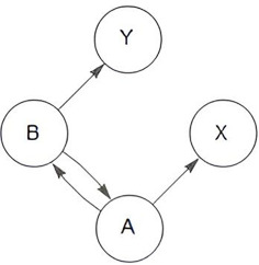
To challenge the validity of axiom 2, we consider the problem of redundancy in a multivariate ecological time-series network, which refers to the presence of excessive and unnecessary causal links among the variables of the network. We can consider a pollination network, which is characterized by mutual interactions [64], and for the sake of simplicity involves only two plant species (A and B) and two pollinators (X and Y). In this system, plant A is pollinated by pollinator X and, plant B by pollinator Y and thus A → X and B → Y. Additionally, a correlation between plant species A and B is also observed so that A ↔ B. However, it is not clear, whether this correlation implies a direct causal relationship between plants A and B, or if there is an indirect relationship through shared pollinators (e.g. X and Y). Consequently, the correlation A ↔ B introduces a problem of redundancy. If axiom 2 is strictly interpreted, and plants A and B are functionally related (owing to a shared pollinator), but this information is redundant, then plant B should be excluded from Ωn. However, excluding B from the set ‘Ωn’ leads to data loss and therefore, the ecological interactions in the pollination network can no longer be revealed.

Finally, we put up the question of whether causal relationships are constant in time (statement 12) by considering the dynamic interactions between Wolbachia (W), mosquito populations (M), disease resistance (R) and their environment (E) [65]. In this example, the presence of Wolbachia in mosquitoes provides disease resistance (W → R). Mosquito populations are affected by disease resistance (R → M). Environment affects both mosquito populations and transmission of Wolbachia (E → M → R). Finally, Wolbachia prevalence is affected by changes in mosquito populations (M → W). Changes in temperature, precipitation or other environmental factors can have a significant impact on mosquito populations and how the system functions. This is possible because the environment can affect breeding sites and mosquito demography, leading to an increase in the proportion of Wolbachia-infected mosquitoes [66].

The complexity of interactions in ecological systems can lead also to the simultaneous or sequential violation of multiple axioms. This is because the density and abundance of organisms often exhibit complex and nonlinear dynamics, which are not constant through time [14]. These dynamics are driven by interactions among organisms, as well as chain, cyclical and multidirectional flows and are particularly evident in scenarios involving certain problematic interaction patterns. For instance, in a three-species food chain (X←Y←Z), it is possible to identify a causal relationship between X and Z [67]. Similarly, in a one-predator–two-prey relationship (X←Z→Y), a causal relationship can be identified between X and Y [68].

5. Statistical limitations of Granger causality in ecological time-series analysis

Without getting into mathematical details, I will briefly discuss here the framework of GC and outline some related statistical challenges that could affect its validity and potentially challenge axiom 1 (statement 5).

Granger causality is based on the concept of conditional probability. It provides the statistical foundation for axiom 1, which is used as a starting point to develop multivariate causal networks. Granger, inspired by the ideas of Suppes [69], who proposed a probabilistic theory of causation, improved his definition of causality for time-series analysis by introducing the concept of prima facie causality ¹ [70]. This allowed him to build a quantifiable definition of causality in which a variable Y causes variable X, if

P(Xn+1 ∈ A|X, Y) ≠ P(Xn+1 ∈ A|X) (13),

for some A X; Y—history of time series: X; Y Xn + 1—the value of X on t+1 [34,43]. Thus, Granger causality relies on conditional probability, comparing two models: one with the past values of both potential cause variable A and potential effect variable C, and another with only the past values of potential effect variable C. Geweke extended Granger causality by introducing a multivariate approach that allows for the identification of conditional Granger causality [71].

To unravel causal relationships among ecosystem components from time-series data, methods like Granger causality must consider essential statistical properties, yet a majority of approaches fail to meet these requirements. I will briefly highlight some of these concerns.

(a). Data stationarity

Conventional statistical tests for linear relationships between non-stationary time series can produce misleading outcomes, known as the ‘spurious regression problem’ [72]. For ecological systems, which often experience various changes over time, appropriate transformations before analysis are essential to avoid erroneous statistical results. Another problem related to stationarity is cointegration, where two or more non-stationary variables exhibit a long-term relationship when combined despite being not correlated in the short run [73]. This violates the independence assumption in time-series analysis and can lead to spurious Granger causality results, where relationships are owing to shared long-term trends rather than genuine causation. Ecological systems often exhibit complex and dynamic behaviour, which can result in non-stationary time-series data [73].

(b). Optimal lag time and autocorrelations

Another challenge that researchers face is choosing the optimal number of lagged observations for regression analysis and controlling for autocorrelation [74]. Autocorrelation can occur in ecological data because ecological systems are often characterized by cyclical or seasonal patterns. If autocorrelation is not removed from the data, it can lead to spurious network results, where GC falsely identifies a causal relationship between any two variables [75]. Addressing this issue requires empirical background knowledge to select suitable lag values and apply methods to control for autocorrelation, such as prewhitening or differencing [17]. However, this information is typically unknown and is part of what the research aims to uncover when studying the system’s behaviour.

(c). Linearity and relevant variables

Granger causality assumes that the actual process generating the data, as well as the causal effects between variables, follow a linear relationship. However, in reality, numerous real-world processes exhibit nonlinearity [57]. This is particularly true for short and noisy time-series data, as they cannot be distinguished from linear processes, making it challenging to extract valuable information. In such cases, nonlinear Granger causality (NGC) should be implemented, which is often conditioned on a large number of confounding variables [76].

(d). Simpson paradox

Simpson’s paradox highlights a phenomenon where the apparent relationship between two variables can change when a third confounding variable is considered. The phenomenon may impact causal reasoning [77] and thus network development, as the relationships between variables in the network can change or become inconsistent when considering different subsets or groupings of the data. This complexity may lead to reversal associations when different datasets or covariates are ignored, complicating the interpretation of data and should be considered in modelling [78,79].

(e). Multiple testing problem

In multivariate Granger causality analysis, the multiple testing problem arises when testing the causal relationships between multiple pairs of variables in a system [80]. As the number of variables increases, so do the number of pairwise combination tests, leading to an increased chance of falsely identifying causal relationships that do not truly exist. Controlling false discovery rates (FDR) helps to strike a balance between detecting true positives (correctly rejecting the null hypothesis when the alternative hypothesis is true) and minimizing the number of false positives [17].

(f). Data quality and sampling frequency

Data quality refers to the assessment of data based on factors such as accuracy, completeness, consistency, reliability and timelines. Ignoring missing data and gaps in the dataset can distort inference [81]. The time scale of a series and the resolution of abundance sampling (i.e. time intervals where sampling is performed) also influences the inherent properties of the dataset [82]. Particularly, they affect the autocorrelations and variance and, consequently, the Granger causality since it traditionally relies on these. Thus, if the data acquisition rate is slower or irregular, it becomes challenging to identify causal effects [83]. Finally, if the sampling frequency is too low, the analysis may only capture short-term fluctuations in the system and miss important long-term trends [84]. This is an important constraint in ecological studies because the selection of sampling frequency can significantly affect the accuracy of study results and can lead to misleading conclusions.

6. The incompleteness of ecological networks as a fundamental property in modelling complex systems

I have already discussed modal logic as a tool for formalizing causal networks to check the degree to which they are violated by known ecological conditions. However, even if no conditions, whether causal rules or statistical properties, are violated, here I outline that it is still impossible to identify all correct causal relationships within an ecological network owing to its inherent properties as a formal system.

By definition, a causal network is a combinatorial object (i.e. discrete mathematical structure), rather than only a geometric one, because the connections between its nodes define it, not only the positions of those nodes in space [85–87]. As a combinatorial object, a causal network is subject to Gödel’s incompleteness theorems. These theorems state that there will always be true statements that are beyond the reach of formal proof and that no formal system can prove its own consistency.

To establish an analogy with Gödel’s incompleteness theorems, we apply them to ecological networks as follows:

The first incompleteness theorem – statement 1: There may be true causal statements about the dynamics of ecological networks that cannot be proven using the rules and axioms of the network. This implies that there will always be some uncertainty regarding how ecological networks will behave, even if we have a thorough understanding of the interactions between the species in the network.

The second incompleteness theorem – statement 2: No formal system (i.e. ecological network) can prove its own consistency. This means that there is always the possibility that the rules and axioms of an ecological network are inconsistent leading to contradictory conclusions.

In the context of ecological networks, based on axioms 1–3 (statements 5–7), I will attempt to formalize the theorems using modal logic as follows:

Axiom 1: There may be true causal statements about the dynamics of ecological networks that cannot be proven using the rules and axioms (1)–(3) of the network, or

◇((A ∧ C) ∧ ¬(A → C)) (14).

Statement (14) asserts that there exists a true causal relationship between A and C in the ecological network (A ∧ C), but it cannot be proven using the rules and axioms of the network (¬(A → C)). This reflects the uncertainty and limitations in fully understanding the causal dynamics of ecological networks.

Axiom 2: No ecological network (i.e. formal system) can prove its own consistency, or

□ (¬ (A → □C)) (15).

This statement negates the possibility of proving the consistency of the ecological network using its own rules and axioms. In other words, the ecological network itself cannot guarantee its own internal coherence (consistency) regarding causal relationships (A → C). In practical terms, statement Axiom 2 (15) states that the relationships and causal interactions should not lead to contradictory or paradoxical conclusions. This highlights the potential for unexpected and unpredictable behaviour in the ecological network owing to its inherent limitations (figure 1).

Figure 1.

Ecological network represented as a formal system (parallelogram) in a Euler diagram. In a complete and consistent system, causal flows are proven true or false, falling within circles of true (T) or false (F) statements. Gödel’s incompleteness theorems introduce undecidable (U) causal flows, lying outside or overlapping the circles. These statements cannot be proven true (or false) using the system's rules and axioms.

A logical proof by contradiction, reductio ad absurdum, of the first statement (1) could be as follows:

1. Assume that axiom 1 (□(P → Q) ∧ □ (¬ (Q → P)) (statement 10) holds in the ecological network.

2. According to axiom 1, if A implies C (A → C), then it cannot be the case that C implies A, or (□ (¬(C →A)).

3. Now, let us consider the causal statement (A → C).

4. Since axiom 1 does not allow ¬ (□(C→A)), it means that there may be uncertainty or limitations in proving the reverse causal relationship.

5. Therefore, ◇((A → C) ∧ □ (¬ (A → C)) holds, implying that there may be true causal statements about the dynamics of ecological networks (A → C) that cannot be proven using the rules and axioms of the network ¬ (□(A → C)).

Following the same logic, we will demonstrate the logical fallacy in axiom 2 (statement (15)). Now we want to show that no ecological network can prove its own consistency regarding causal relationships:

1. Let us assume that an ecological network can prove its own consistency, which means that (A → □C) is true and provable within the network.

2. According to axiom 3 (□(P → Q)), if a variable P caused Q at time t (P → Q), then P will still cause Q at any future time t + i (□(P → Q)).

3. In the context of the ecological network, the causal relationship between variables (A → C) is considered consistent and provable (□(A → C)).

4. However, this leads to a contradiction with axiom 1 (□(P → Q) ∧ □(¬ (Q → P)). If we replace P with A and Q with C, we get: □(A → C) ∧ □(¬ (C → A)).

5. The contradiction arises from the inconsistency between □(A → C) and □ (¬(C → A)), meaning that the ecological network cannot simultaneously prove the consistency of (A → C) and its inverse (C → A).

6. Therefore, the assumption that we have used as a starting point that the ecological network can prove its own consistency (A → □C) is false, and we have □ (¬ (A → □C)).

The above formalizations capture the essence of Gödel’s incompleteness theorems in the context of ecological networks. Yet, before closing, we should also address some potential critiques of the established analogy between ecological networks as formal systems and the use of incompleteness theorems to outline their limitations. For instance, ecological interactions are quite complex to the degree that they cannot be fully described in terms of formal logic, while the proofs rely on particular axioms with respect to counterfactual causality and might not be relevant to all ecological networks. The answer to the first critique is that since the network is formalized into discrete mathematics its properties will follow the rules of incompleteness theorems. Regarding the second argument, that is, the interpretation is based on specific rules or postulates, the counterargument is that we could increase the axioms in order to prove more causal statements. However, whenever we add axioms there will always be true interactions that cannot be proved within the system. Additionally, there will always be the case of axioms that contradict each other because of incompleteness theorems. Ultimately, we will always need more information to fully understand a complex system from sources outside the system under consideration.

Finally, despite ecological networks not conforming to the strictest definition of self-reference, where incompleteness theorems become prominent, they do exhibit self-referential properties at an emergent level, as evidenced by the definition of causality using symbolic logic and the examples provided. Notably, evolutionary networks display a pronounced self-referential quality. For instance, coevolutionary changes in traits driven by mutualistic symbiosis between species and the influence of immunity on disease transmission dynamics within a disease network demonstrate self-referential aspects of the ecological network. Consequently, ecological networks inherently involve circularity or dynamic reflexivity, giving rise to emergent properties and behaviours that defy simple rule-based explanation or prediction, making the concept of incompleteness relevant to ecological network modelling.

Ethics

This work did not require ethical approval from a human subject or animal welfare committee.

Data accessibility

This article has no additional data.

Declaration of AI use

AI software was used to translate and/or correct grammar and spelling to improve readability and refine the language in some parts of the text.

Authors’ contributions

P.T.D.: conceptualization, formal analysis, investigation, methodology, software, writing—original draft, writing—review and editing.

Conflict of interest declaration

I declare I have no competing interests.

Funding

No funding has been received for this article.

References

- 1. Landi P, Minoarivelo HO, Brännström Å, Hui C, Dieckmann U. 2018. Complexity and stability of ecological networks: a review of the theory. Popul. Ecol. 60 , 319–345. ( 10.1007/s10144-018-0628-3) [DOI] [Google Scholar]
- 2. Guimarães Jr PR. 2020. The structure of ecological networks across levels of organization. Annu. Rev. Ecol. Evol. Syst. 51 , 433–460. ( 10.1146/annurev-ecolsys-012220-120819) [DOI] [Google Scholar]
- 3. Segar ST, Fayle TM, Srivastava DS, Lewinsohn TM, Lewis OT, Novotny V, Kitching RL, Maunsell SC. 2020. The role of evolution in shaping ecological networks. Trends Ecol. Evol. 35 , 454–466. ( 10.1016/j.tree.2020.01.004) [DOI] [PubMed] [Google Scholar]
- 4. May RM. 1972. Will a large complex system be stable? Nature 238 , 413–414. ( 10.1038/238413a0) [DOI] [PubMed] [Google Scholar]
- 5. Dunne JA, Williams RJ, Martinez ND. 2002. Network structure and biodiversity loss in food webs: robustness increases with connectance. Ecol. Lett. 5 , 558–567. ( 10.1046/j.1461-0248.2002.00354.x) [DOI] [Google Scholar]
- 6. Williams-García RV, Beggs JM, Ortiz G. 2017. Unveiling causal activity of complex networks. Europhys. Lett. 119 , 18003. ( 10.1209/0295-5075/119/18003) [DOI] [Google Scholar]
- 7. Solvang HK, Subbey S. 2019. An improved methodology for quantifying causality in complex ecological systems. PLoS One 14 , e0208078. ( 10.1371/journal.pone.0208078) [DOI] [PMC free article] [PubMed] [Google Scholar]
- 8. Geary WL, Bode M, Doherty TS, Fulton EA, Nimmo DG, Tulloch AIT, Tulloch VJD, Ritchie EG. 2020. A guide to ecosystem models and their environmental applications. Nat. Ecol. Evol. 4 , 1459–1471. ( 10.1038/s41559-020-01298-8) [DOI] [PubMed] [Google Scholar]
- 9. Runge J, Nowack P, Kretschmer M, Flaxman S, Sejdinovic D. 2017. Detecting and quantifying causal associations in large nonlinear time series datasets. Sci. Adv. 27 , eaau4996. ( 10.1126/sciadv.aau4996) [DOI] [PMC free article] [PubMed] [Google Scholar]
- 10. Barigozzi M, Brownlees C. 2019. NETS: network estimation for time series. J. Appl Econ. 34 , 347–364. ( 10.1002/jae.2676) [DOI] [Google Scholar]
- 11. Chang CW, et al. 2022. Causal networks of phytoplankton diversity and biomass are modulated by environmental context. Nat. Commun. 13 , 1140. ( 10.1038/s41467-022-28761-3) [DOI] [PMC free article] [PubMed] [Google Scholar]
- 12. Krabbe Borregaard M, Rahbek C. 2010. Causality of the relationship between geographic distribution and species abundance. Q. Rev. Biol. 85 , 41–78. ( 10.1086/650265) [DOI] [PubMed] [Google Scholar]
- 13. Godfrey SS. 2013. Networks and the ecology of parasite transmission: a framework for wildlife parasitology. Int. J. Parasitol. Parasites Wildl. 2 , 235–245. ( 10.1016/j.ijppaw.2013.09.001) [DOI] [PMC free article] [PubMed] [Google Scholar]
- 14. Suzuki K, Matsuzaki S, Masuya H. 2022. Decomposing predictability to identify dominant causal drivers in complex ecosystems. Proc. Natl. Acad. Sci. USA 119 , e2204405119. ( 10.1073/pnas.2204405119) [DOI] [PMC free article] [PubMed] [Google Scholar]
- 15. Frossard V, Rimet F, Perga ME. 2018. Causal networks reveal the dominance of bottom-up interactions in large, deep lakes. Ecol. Modell. 368 , 136–146. ( 10.1016/j.ecolmodel.2017.11.021) [DOI] [Google Scholar]
- 16. Li J, Convertino M. 2021. Inferring ecosystem networks as information flows. Sci. Rep. 11 , 7094. ( 10.1038/s41598-021-86476-9) [DOI] [PMC free article] [PubMed] [Google Scholar]
- 17. Damos P. 2016. Using multivariate cross correlations, Granger causality and graphical models to quantify spatiotemporal synchronization and causality between pest populations. BMC Ecol. 16 , 33. ( 10.1186/s12898-016-0087-7) [DOI] [PMC free article] [PubMed] [Google Scholar]
- 18. Sandberg CL, Clack CD. 2021. Incorporation of causality structures to complex network analysis of time-varying behaviour of multivariate time series. Sci. Rep. 11 , 18880. ( 10.1038/s41598-021-97741-2) [DOI] [PMC free article] [PubMed] [Google Scholar]
- 19. Krakovská A, Jakubík J, Chvosteková M, Coufal D, Jajcay N, Paluš M. 2018. Comparison of six methods for the detection of causality in a bivariate time series. Phys. Rev. E 97 , 042207. ( 10.1103/PhysRevE.97.042207) [DOI] [PubMed] [Google Scholar]
- 20. Granger CWJ. 1969. Investigating causal relations by econometric models and cross-spectral methods. Econometrica 37 , 424–438. ( 10.2307/1912791) [DOI] [Google Scholar]
- 21. Granger CWJ. 1988. Causality, cointegration, and control. J. Econ. Dyn. Control 12 , 551–559. ( 10.1016/0165-1889(88)90055-3) [DOI] [Google Scholar]
- 22. Gödel K. 1931. Über formal unentscheidbare Sätze der Principia Mathematica und verwandter Systeme I. Monatsh. Math. Physik 38–38 , 173–198. ( 10.1007/BF01700692) [DOI] [Google Scholar]
- 23. Raatikainen P. 2018. Gödel’s incompleteness Theorems. In The Stanford encyclopedia of philosophy (fall 2018 edition) (ed. Zalta EN). Stanford, CA: Stanford University. [Google Scholar]
- 24. Raj U, Upadhyay S, Karmakar M, Bhattacharya S. 2022. Simplicial structures in ecological networks. arXiv. ( 10.48550/arXiv.2203.13677) [DOI]
- 25. Levins R, Schultz BB. 1996. Effects of density dependence, feedback and environmental sensitivity on correlations among predators, prey and plant resources: models and practical implications. J. Anim. Ecol. 65 , 802–812. ( 10.2307/5678) [DOI] [Google Scholar]
- 26. Levins R, Puccia CJ. 1988. The controlling factor in biological communities. Coenoses 3 , 149–154. [Google Scholar]
- 27. Halpern JY, Pearl J. 2005. Causes and explanations: a structural-model approach. Part I: causes. Br. J. Philos. Sci. 56 , 843–887. ( 10.1093/bjps/axi147) [DOI] [Google Scholar]
- 28. Pearl J. 2010. An introduction to causal inference. Int. J. Biostat. 6 . ( 10.2202/1557-4679.1203) [DOI] [PMC free article] [PubMed] [Google Scholar]
- 29. Imbens GW, Rubin DB. 2010. Rubin causal model. In Microeconometrics. The new Palgrave economics collection (eds Durlauf SN, Blume LE). London, UK: Palgrave Macmillan. ( 10.1057/9780230280816) [DOI] [Google Scholar]
- 30. Tucci RR. 2013. Introduction to Judea pearl’s do-Calculus. arXiv. ( 10.48550/arXiv.1305.5506) [DOI]
- 31. Qian SS, Craig JK, Baustian MM, Rabalais NN. 2009. A Bayesian hierarchical modeling approach for analyzing observational data from marine ecological studies. Mar. Pollut. Bull. 58 , 1916–1921. ( 10.1016/j.marpolbul.2009.09.029) [DOI] [PubMed] [Google Scholar]
- 32. Barbero F, Schulz K, Smets S, Velázquez-Quesada FR, Xie K. Thinking about causation: a causal language with epistemic operators. In Proc. 3rd Int. Worksh. Dynamic Logic (DaLí ’20) (eds MA Martins, I Sedl´ar), pp. 17–32. Heidelberg, Germany: Springer. [Google Scholar]
- 33. Kawamoto Y, Sato T, Suenaga K. 2013. Formalizing statistical causality via modal logic. arXiv. ( 10.48550/arXiv.2210.16751) [DOI]
- 34. Stern CD. 1981. Lewis’ counterfactual analysis of causation. Synthese 48 , 333–345. ( 10.1007/BF01063984) [DOI] [Google Scholar]
- 35. Bernstein S. 2019. Lewis’s theories of causation and their influence. In The Cambridge history of philosophy, 1945–2015 (eds Becker K, Thomson ID), pp. 160–170. Cambridge, UK: Cambridge University Press. ( 10.1017/9781316779651) [DOI] [Google Scholar]
- 36. Hughes GE, Cresswell MJ. 1968. An introduction to modal logic. London, UK: Methuen and Co. Ltd. [Google Scholar]
- 37. Gabbay D. 1969. Saul A. Kripke. Semantical considerations for modal logics. Proceedings of a colloquium on modal and many-valued logics, Helsinki, 23-26 August, 1962, Acta Philosophica Fennica 1963, pp. 83–94. J. Symbol. Logic. 34, 501. ( 10.2307/2270922) [DOI] [Google Scholar]
- 38. Lewis DK. 1986. On the plurality of worlds. Oxford, UK: Blackwell. [Google Scholar]
- 39. Richardson M, Domingos P. 2006. Markov logic networks. Mach. Learn. 62 , 107–136. ( 10.1007/s10994-006-5833-1) [DOI] [Google Scholar]
- 40. Kaveh A, Magnani M, Rohner C. 2021. Defining and measuring probabilistic ego networks. Soc. Netw. Anal. Min. 11 , 25. ( 10.1007/s13278-020-00708-w) [DOI] [Google Scholar]
- 41. Kment B. 2020. Counterfactuals and causal reasoning. In Perspectives on causation (eds Bar-Asher Siegal EA, Boneth N), pp. 463–482. Heidelberg, Germany: Springer. ( 10.1007/978-3-030-34308-8) [DOI] [Google Scholar]
- 42. Pearl J. 2000. Correlation and causality: models, reasoning, and inference. Cambridge, UK: Cambridge University Press. [Google Scholar]
- 43. Maziarz M. 2015. A review of the Granger-causality fallacy. J. Philos. Econ. 8 , 86–105. ( 10.46298/jpe.10676) [DOI] [Google Scholar]
- 44. Pausas JG, Bond WJ. 2022. Feedbacks in ecology and evolution. Trends Ecol. Evol. 37 , 211–222. ( 10.1016/j.tree.2022.03.008) [DOI] [PubMed] [Google Scholar]
- 45. Burton PJ, Jentsch A, Walker LR. 2020. The ecology of disturbance interactions. Bioscience 70 , 854–870. ( 10.1093/biosci/biaa088) [DOI] [Google Scholar]
- 46. Baldwin JM. 1897. Organic selection. Science 5 , 634–636. ( 10.1126/science.5.121.634) [DOI] [PubMed] [Google Scholar]
- 47. Crispo E. 2007. The Baldwin effect and genetic assimilation: revisiting two mechanisms of evolutionary change mediated by phenotypic plasticity. Evolution. 61 , 2469–2479. ( 10.1111/j.1558-5646.2007.00203.x) [DOI] [PubMed] [Google Scholar]
- 48. Russell B. 1912. The problems of philosophy. London, UK: William & Norgate. [Google Scholar]
- 49. Holling CS. 1973. Resilience and stability of ecological systems. Annu. Rev. Ecol. Syst. 4 , 1–23. ( 10.1146/annurev.es.04.110173.000245) [DOI] [Google Scholar]
- 50. Newman EA, Kennedy MC, Falk DA, McKenzie D. 2019. Scaling and complexity in landscape ecology. Front. Ecol. Evol. 7 , 293. ( 10.3389/fevo.2019.00293) [DOI] [Google Scholar]
- 51. Banitz T, Schlüter M, Lindkvist E, Radosavljevic S, Johansson LG, Ylikoski P, Martínez-Peña R, Grimm V. 2022. Model-derived causal explanations are inherently constrained by hidden assumptions and context: the example of Baltic cod dynamics. Environ. Model. Softw. 156 , 105489. ( 10.1016/j.envsoft.2022.105489) [DOI] [Google Scholar]
- 52. Hamilton JD. 1989. A new approach to the economic analysis of nonstationary time series and the business cycle. Econometrica 57 , 357–384. ( 10.2307/1912559) [DOI] [Google Scholar]
- 53. Friston K, Moran R, Seth AK. 2013. Analysing connectivity with Granger causality and dynamic causal modelling. Curr. Opin. Neurobiol. 23 , 172–178. ( 10.1016/j.conb.2012.11.010) [DOI] [PMC free article] [PubMed] [Google Scholar]
- 54. Zhao S, Zhang J. 2022. Causal effect of the tropical Pacific sea surface temperature on the Upper Colorado River Basin spring precipitation. Clim. Dyn. 58 , 941–959. ( 10.1007/s00382-021-05944-0) [DOI] [Google Scholar]
- 55. Mainali K, Bewick S, Vecchio-Pagan B, Karig D, Fagan WF. 2019. Detecting interaction networks in the human microbiome with conditional Granger causality. PLoS Comput. Biol. 15 , e1007037. ( 10.1371/journal.pcbi.1007037) [DOI] [PMC free article] [PubMed] [Google Scholar]
- 56. Barraquand F, Picoche C, Detto M, Hartig F. 2021. Inferring species interactions using Granger causality and convergent cross mapping. Theor. Ecol. 14 , 87–105. ( 10.1007/s12080-020-00482-7) [DOI] [Google Scholar]
- 57. Shojaie A, Fox EB. 2022. Granger causality: a review and recent advances. Annu. Rev. Stat. Appl. 9 , 289–319. ( 10.1146/annurev-statistics-040120-010930) [DOI] [PMC free article] [PubMed] [Google Scholar]
- 58. Wiener N. 1956. The theory of prediction. In Modern mathematics for engineers (ed. Beckenbach EF), pp. 165–190. New York, NY: McGraw-Hill. [Google Scholar]
- 59. Hume D. 1978. A treatise of human nature. In British moralists, 1650–1800. Indianapolis, IN: Hackett Publishing. [Google Scholar]
- 60. Granger CWJ. 1980. Testing for causality. A personal viewpoint. J. Econ. Dynamic Control 2 , 329–352. ( 10.1016/0165-1889(80)90069-X) [DOI] [Google Scholar]
- 61. Roy S, Chattopadhyay J. 2007. The stability of ecosystems: a brief overview of the paradox of enrichment. J. Biosci. 32 , 421–428. ( 10.1007/s12038-007-0040-1) [DOI] [PubMed] [Google Scholar]
- 62. Gallien L, Zimmermann NE, Levine JM, Adler PB. 2017. The effects of Intransitive competition on coexistence. Ecol. Lett. 20 , 791–800. ( 10.1111/ele.12775) [DOI] [PubMed] [Google Scholar]
- 63. Cardinale BJ, Weis JJ, Forbes AE, Tilmon KJ, Ives AR. 2006. Biodiversity as both a cause and consequence of resource availability: a study of reciprocal causality in a predator–prey system. J. Anim. Ecol. 75 , 497–505. ( 10.1111/j.1365-2656.2006.01070.x) [DOI] [PubMed] [Google Scholar]
- 64. Bascompte J, Jordano P. 2007. Plant–animal mutualistic networks: the architecture of biodiversity. Annu. Rev. Ecol. Evol. Syst. 38 , 567–593. ( 10.1146/annurev.ecolsys.38.091206.095818) [DOI] [Google Scholar]
- 65. Zélé F, Nicot A, Berthomieu A, Weill M, Duron O, Rivero A. 2014. Wolbachia increases susceptibility to plasmodium infection in a natural system. Proc. Biol. Sci. 281 , 20132837. ( 10.1098/rspb.2013.2837) [DOI] [PMC free article] [PubMed] [Google Scholar]
- 66. Damos P, Caballero P. 2021. Detecting seasonal transient correlations between populations of the West Nile Virus vector Culex sp. and temperatures with wavelet coherence analysis. Ecol. Inform. 61 , 101216. ( 10.1016/j.ecoinf.2021.101216) [DOI] [Google Scholar]
- 67. Ye H, Deyle ER, Gilarranz LJ, Sugihara G. 2015. Distinguishing time-delayed causal interactions using convergent cross mapping. Sci. Rep. 5 , 14750. ( 10.1038/srep14750) [DOI] [PMC free article] [PubMed] [Google Scholar]
- 68. Leng S, Ma H, Kurths J, Lai YC, Lin W, Aihara K, Chen L. 2020. Partial cross mapping eliminates indirect causal influences. Nat. Commun. 11 , 2632. ( 10.1038/s41467-020-16238-0) [DOI] [PMC free article] [PubMed] [Google Scholar]
- 69. Suppes P. 1970. A probabilistic theory of causality. Acta Philos. Fenn. 24 , 130. [Google Scholar]
- 70. Davis WA. 1988. Probabilistic theories of causation. In Probability and causality (ed. Fetzer JH), vol. 192. Dordrecht, The Netherlands: Springer. ( 10.1007/978-94-009-3997-4) [DOI] [Google Scholar]
- 71. Geweke J. 1982. Measurement of linear dependence and feedback between multiple time series. J. Am. Stat. Assoc. 77 , 304–313. ( 10.1080/01621459.1982.10477803) [DOI] [Google Scholar]
- 72. Granger CWJ, Newbold P. 1974. Spurious regressions in econometrics. J. Econom. 2 , 111–120. ( 10.1016/0304-4076(74)90034-7) [DOI] [Google Scholar]
- 73. Gao X, Huang S, Sun X, Hao X, An F. 2018. Modelling cointegration and Granger causality network to detect long-term equilibrium and diffusion paths in the financial system. R. Soc. Open Sci. 5 , 172092. ( 10.1098/rsos.172092) [DOI] [PMC free article] [PubMed] [Google Scholar]
- 74. Arbabshirani MR, et al. 2014. Impact of autocorrelation on functional connectivity. Neuroimage 102 , 294–308. ( 10.1016/j.neuroimage.2014.07.045) [DOI] [PMC free article] [PubMed] [Google Scholar]
- 75. Chiarion G, Sparacino L, Antonacci Y, Faes L, Mesin L. 2023. Connectivity analysis in EEG data: a tutorial review of the state of the art and emerging trends. Bioengineering 10 , 372. ( 10.3390/bioengineering10030372) [DOI] [PMC free article] [PubMed] [Google Scholar]
- 76. Chen Y, Rangarajan G, Feng J, Ding M. 2004. Analyzing multiple nonlinear time series with extended Granger causality. Phys. Lett. A 324 , 26–35. ( 10.1016/j.physleta.2004.02.032) [DOI] [Google Scholar]
- 77. Neufeld E. 1995. Simpson’s paradox in artificial intelligence and in real life. Comput. Intell. 11 , 1–10. ( 10.1111/j.1467-8640.1995.tb00021.x) [DOI] [Google Scholar]
- 78. Appleton DR, French JM, Vanderpump MPJ. 1996. Ignoring a covariate: an example of Simpson’s paradox. Am. Stat. 50 , 340–341. ( 10.1080/00031305.1996.10473563) [DOI] [Google Scholar]
- 79. Holmes EE, Scheuerelland MD, Ward EJ. 2023. Analysis of multivariate time series using the MARSS package, version 3.11.4, pp. 98–112. Seattle, WA: NOAA. [Google Scholar]
- 80. Yu L. 2021. False discovery rates in biological networks. In Proc. 24th Int. Conf. Artificial Intelligence and Statistics (AISTATS), San Diego, California, USA. [Google Scholar]
- 81. Łopucki R, Kiersztyn A, Pitucha G, Kitowski I. 2022. Handling missing data in ecological studies: ignoring gaps in the dataset can distort the inference. Ecol. Modell. 468 , 109964. ( 10.1016/j.ecolmodel.2022.109964) [DOI] [Google Scholar]
- 82. Arkilanian AA, Clements CF, Ozgul A, Baruah G. 2020. Effect of time series length and resolution on abundance- and trait-based early warning signals of population declines. Ecology 101 , e03040. ( 10.1002/ecy.3040) [DOI] [PubMed] [Google Scholar]
- 83. Pyper BJ, Peterman RM. 1998. Comparison of methods to account for autocorrelation in correlation analyses of fish data. Can. J. Fish. Aquat. Sci. 55 , 2127–2140. ( 10.1139/f98-104) [DOI] [Google Scholar]
- 84. Bruel R, White ER. 2021. Sampling requirements and approaches to detect ecosystem shifts. Ecol. Indic. 121 , 107096. ( 10.1016/j.ecolind.2020.107096) [DOI] [Google Scholar]
- 85. Erdös P. 2016. Some remarks on the theory of graphs. Bull. Amer. Math. Soc. 53 , 292–294. ( 10.1090/S0002-9904-1947-08785-1) [DOI] [Google Scholar]
- 86. Chung F, Lu L. 2006. Complex graphs and networks. Providence, RI: AMS.(CBMS Regional Conference Series in Mathematics). ( 10.1090/cbms/107) [DOI] [Google Scholar]
- 87. Harris J, Hirst JL, Mossinghoff M. 2008. Combinatorics and graph theory. New York, NY: Springer. ( 10.1007/978-0-387-79711-3) [DOI] [Google Scholar]
Associated Data
This section collects any data citations, data availability statements, or supplementary materials included in this article.
Data Availability Statement