HornBase: An audio dataset of car horns in different scenarios and positions

Abstract

In recent years, there has been significant growth in the development of Machine Learning (ML) models across various fields, such as image and sound recognition and natural language processing. They need to be trained with a large enough data set, ensuring predictions or results are as accurate as possible. When it comes to models for audio recognition, specifically the detection of car horns, the datasets are generally not built considering the specificities of the different scenarios that may exist in real traffic, being limited to collections of random horns, whose sources are sometimes collected from audio streaming sites. There are benefits associated with a ML model trained on data tailored for horn detection. One notable advantage is the potential implementation of horn detection in smartphones and smartwatches equipped with embedded models to aid hearing-impaired individuals while driving and alert them in potentially hazardous situations, thus promoting social inclusion. Given these considerations, we developed a dataset specifically for car horns. This dataset has 1,080 one-second-long .wav audio files categorized into two classes: horn and not horn. The data collection followed a carefully established protocol designed to encompass different scenarios in a real traffic environment, considering diverse relative positions between the involved vehicles. The protocol defines ten distinct scenarios, incorporating variables within the car receiving the horn, including the presence of internal conversations, music, open or closed windows, engine status (on or off), and whether the car is stationary or in motion. Additionally, there are variations in scenarios associated with the vehicle emitting the horn, such as its relative position—behind, alongside, or in front of the receiving vehicle—and the types of horns used, which may include a short honk, a prolonged one, or a rhythmic pattern of three quick honks. The data collection process started with simultaneous audio recordings on two smartphones positioned inside the receiving vehicle, capturing all scenarios in a single audio file on each device. A 400-meter route was defined in a controlled area, so the audio recordings could be carried out safely. For each established scenario, the route was covered with emissions of different types of horns in distinct positions between the vehicles, and then the route was restarted in the next scenario. After the collection phase, the data preprocessing involved manually cutting each horn sound in multiple one-second windowing profiles, saving them in PCM stereo .wav files with a 16-bit depth and a 44.1 kHz sampling rate. For each horn clipping, a corresponding non-horn clipping in close proximity was performed, ensuring a balanced model. This dataset was designed for utilization in various machine learning algorithms, whether for detecting horns with the binary labels, or classifying different patterns of horns by rearranging labels considering the file nomenclature. In technical validation, classifications were performed using a convolutional neural network trained with spectrograms from the dataset's audio, achieving an average accuracy of 89% across 100 trained models.

Specifications Table

Subject	Computer Science/Artificial Intelligence
Specific subject area	The dataset can be used to train binary and multi-class ML classifier models to detect the presence or absence of sound from three types of horns.
Type of data	Raw Audio Excerpts (.wav format)
Data collection	The dataset comprises 1,080 audio files, each with a precise one-second time window and a nomenclature that identifies whether it is a horn or not, its type, the relative position of the vehicles, and the displacement of the clipping window. The dataset is balanced. The collection process involved two vehicles, one emitting horns and the other receiving them while covering a route for each defined scenario. In the receiving vehicle, two Android smartphones were placed for audio recordings in .wav format, with a 16-bit depth and a 44.1 kHz sampling rate. The data underwent preprocessing through manual cutting of audio segments with and without horns using the Audacity 3.3.2 software.
Data source location	Institution: Federal University of Para - Guamá Science and Technology Park City: Belem – Para Country: Brazil Latitude and Longitude: -1.46465, -48.44318
Data accessibility	Repository name: Mendeley Data Digital Object Identifier: 10.17632/y5stjsnp8s.2 Direct URL to data: https://data.mendeley.com/datasets/y5stjsnp8s/2

1. Value of the Data

• •This is a dataset composed of horn and not-horn sounds, maintaining class balance in the set. Its creation involved scenario-driven data collection, considering situations encountered in a real traffic environment. No specific horn datasets were found in the literature available in academic databases such as IEEE, ACM Digital Library, and ScienceDirect when searching for ``horn'' and ``dataset'' or ``honk'' and ``dataset''. The available datasets containing horn sounds are typically compilations of various types of sounds collected from online sound platforms. Therefore, this is potentially a unique dataset due to its distinctive characteristics.
• •We believe that the dataset might be useful for horn detection research involving Machine Learning (ML) by providing raw data for feature extraction (mel-frequency cepstral coefficients, spectrograms, among others) and model design. In this manner, it brings positive impacts to the academic field.
• •From a social point of view, the construction and availability of this database can encourage and provide inputs for potential research on social inclusion through the detection of car horns in traffic environments for the hearing-impaired. This scene would potentially be achieved through intelligent models embedded in smartphones and smartwatches, for instance.
• •The dataset is structured following a specific nomenclature to differentiate each scenario, vehicle position, horn type, horn occurrence, and audio clipping window displacement. The latter is important to ensure that ML models have examples of audio snippets playing only the beginning of a horn or just the ending, situations that may occur in real-time detection.
• •Given that the vehicles are moving in most collection scenarios, a distinctive aspect of this dataset is the occurrence of audio with and without the Doppler effect, which can have a significant impact on models for horn detection. This is because the sound's frequency emitted by a moving source are perceived differently by the receiver [1], leading to potential changes in the features extracted from the audio. A model trained with this dataset may possibly learn differences between sounds emitted by stationary and moving vehicles.
• •As the variation in the distance between the two moving vehicles interferes with the audio waveform, it is important not to fix it during the data collection. The dataset needs to include a variety of examples to prevent biasing models towards specific configurations. Therefore, the proposed database was constructed with random distances in each scenario.

2. Background

In previous research [2,3], the requirement for a specialized horn dataset to train machine learning models that account for diverse scenarios in a real traffic environment was recognized. The ultimate objective is to incorporate individuals with hearing impairments into traffic considerations. Although there are datasets in the literature that contain horns, such as UrbanSound [4], ESC [5], and FSD50K [6], they are not specific sets for this task, as their data have been collected from online platforms.

Additionally, audio datasets collected by the authors themselves in real environments or situations were observed. Examples include the Chime-Home [7], a dataset of gunshot audio [8], one focused on motor sounds [9], and some specific resources for spoken tasks, such as AudioMNIST [10] and STOP [11]. Also, there are audio datasets created through cutting, modifications, and transformations applied to existing datasets, such as SARdB [12] for audio scenes and Shrutilipi [13] for automatic speech recognition. Although none of them pertain to horns, they provide guides for the creation of a collection protocol.

3. Data Description

This dataset consists of 1,080 audio files in raw .wav format with a 16-bit depth and a 44.1 kHz sampling rate - common recording and editing formats typically found in the literature - each with a one-second time interval. It is divided into two classes, comprising 540 horn and 540 not-horn files. These files are located within the Dataset folder, which has been compressed into the Dataset.zip file.

The hornbase.csv file lists all the .wav files with their respective labels (horn or not-horn) and corresponding numerical values (1 and 0, respectively). Additionally, there are the hornbase_train.csv and hornbase_test.csv files, maintaining the structure of the hornbase.csv file but dividing the main dataset in a 70/30 ratio for train and test, respectively.

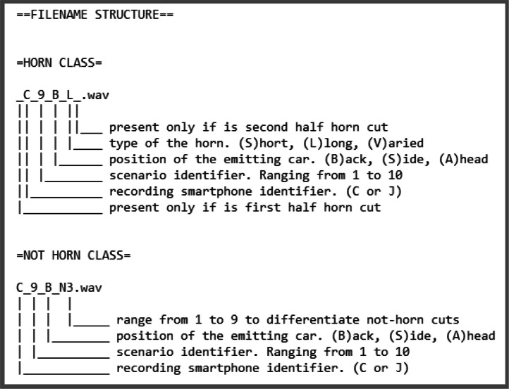
There is also a file that describes the nomenclature of the audio files, providing information about the recording device, whether it is a horn or not, the relative position of the vehicles, the horn type, and the displacement of the clipping window. This can be useful in situations where the researcher wants to extend binary labeling to also encompass the type of horn, for instance. The proposed nomenclature is shown in Fig. 1.

Fig. 1.

HornBase filename structure.

4. Experimental Design, Materials and Methods

We defined a careful data collection protocol, outlining the possible scenarios and positions of the vehicles involved, the materials needed to collect the audio, the streets for the collection route, and the honking styles. Then, the processing and labeling protocol used to orchestrate the audio cutting and organize the file structure of the dataset was defined.

4.1. Data Collection Protocol

The first step involved defining different possible scenarios for receiving sounds inside a car. Consequently, ten situations were identified regarding the receiving vehicle: Car engine on and off, with or without music, people conversing or in silence, car with open or closed windows, stationary or moving car. Additionally, variations in the relative position of the cars were defined, including the emitter behind, alongside, or in front of the receiver.

Engine-on or engine-off scenarios were established because a horn can be received while the car is running, or while it is parked about to start. So the engine noise can be captured together with the horn and harms its recognition. The same principle applies to scenarios of music or any other sound coming from the car's speakers. Likewise, internal conversations may reduce the quality of the received sound. So all these variations must be considered when training the model.

The window's open or closed scenario is also related to the quality of the sound that will be recorded. An open window can facilitate the capture of an outside sound, but it will also increase the presence of noises from other vehicles and ambient sounds. The closed window keeps the car's environment more isolated and with a different acoustics. Therefore, it is valid to have examples of these two profiles in the dataset.

This approach resulted in ten collection scenarios, each one involving a variation of three relative positions between the vehicles. In each position, three types of horns were sounded: A short horn, a long horn, and a rhythmic three-honk horn. Table. 1 presents the ten chosen scenarios.

Table 1.

Receiver vehicle scenarios.

Identifier	Description
Scenario 01	Car with windows closed, engine off, sound off, no internal conversations
Scenario 02	Car with windows closed, engine running, sound off, no internal conversations, no movement
Scenario 03	Car with windows closed, engine running, sound off, no internal conversations, in motion
Scenario 04	Car with windows closed, engine running, sound on, no internal conversations, in motion
Scenario 05	Car with windows open, engine running, sound off, no internal conversations, in motion
Scenario 06	Car with windows closed, engine running, sound off, with internal conversations, in motion
Scenario 07	Car with windows closed, engine running, sound on, with internal conversations, in motion
Scenario 08	Car with windows open, engine running, sound on, no internal conversations, in motion
Scenario 09	Car with windows open, engine running, sound off, with internal conversations, in motion
Scenario 10	Car with windows open, engine running, sound on, with internal conversations, in motion

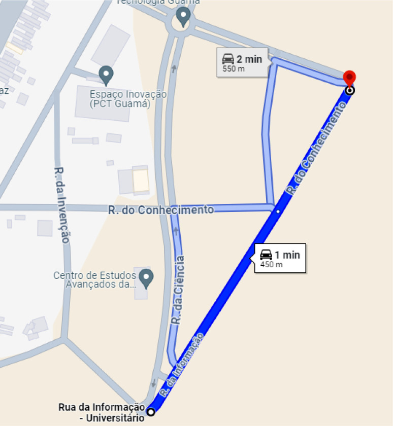
With the scenarios defined, the location for data collection was decided: For safety reasons, an isolated street at a university, on a straight route of 450 meters. In each scenario, the cars traveled along the chosen street, totaling ten round trips. Fig. 2 shows the chosen route.

Fig. 2.

The chosen route for data collection.

The next step was to define the materials necessary for data collection, in audio format in this case. For the procedure, two cars must be available, one to emit the horns, and the other will be the horn receiver where the audio recording devices will be located. The devices chosen for this task were two android smartphones of different models so that there would be audio from different recording sources in the dataset. The Super Recorder App was chosen to continuously record high-quality, lossless stereo audio in .wav format.

The data collection process began by starting audio recording on both smartphones, with the horns being emitted in the appropriate positions of the cars. The distance between vehicles was not specified when the emitter was either behind or ahead, as maintaining constant precision would be challenging while the cars were in motion. Anyway, the distance ranged from 30 to 80 meters. When the vehicles were positioned side by side, the distance varied from two to five meters. At the end of the collection, two .wav audio files, each lasting approximately 18 minutes, were obtained, which were cut and processed in the next phase.

4.2. Processing and Labeling Protocol

In order to process the two audio files and extract excerpts, we opted for the software Audacity due to its user-friendly interface for manipulating waveforms. Initially, the ten recorded scenarios were cut from each file and named with the corresponding number, along with a smartphone identifier, resulting in a total of 20 scenario files.

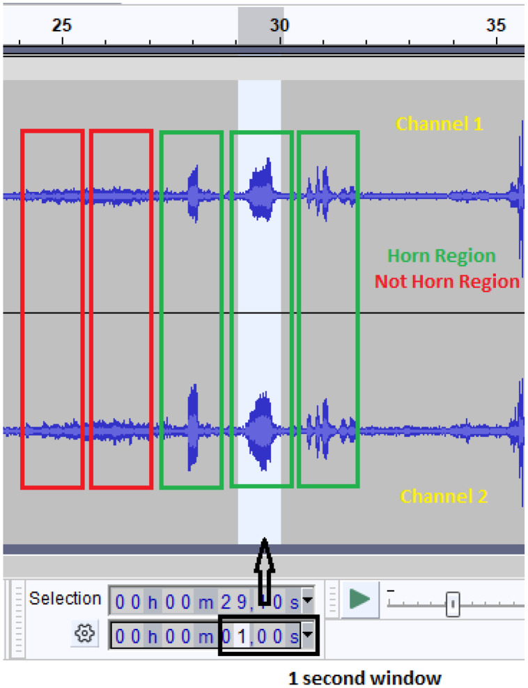
The audio files were then individually listened to and the respective waveforms examined with the aim of identifying segments with and without horn sounds. Once the horn was located, we selected three sections (or parts): The first part covering the entire horn duration; the second covering half of the sound, starting 500ms before the first part; and a third covering the other half of the sound, ending 500ms after the first part. Each section strictly lasted one second.

For every horn-containing section, we extracted a corresponding one-second section without a horn nearby, establishing a balanced binary class scheme. Fig. 3 illustrates part of the Audacity interface, highlighting regions with different horn sounds in green (short, long, and varying, from left to right), areas without horns in red, and the clipping area.

Fig. 3.

The audio cutting process in the Audacity software.

The label of an audio, whether of the horn class or the non-horn class, was defined at the time of the clipping itself, since it was already known at this point which class the audio belonged to. The note was made in the name of the file itself when saving it, through the nomenclature X_N_Y_Z for cases in which there is an occurrence of a horn, where:

• •X is the smartphone identifier (C or J);
• •N is the scenario identifier number (ranging from one to ten);
• •Y represents the position of the emitting vehicle in relation to the receiver (B for back, S for side, A for ahead) and;
• •Z represents the horn type (S for short, L for long, V for varied).

Thus, the file C_9_B_L, for example, refers to a clipping obtained from the smartphone labeled as C, ninth scenario, when the emitting vehicle was behind the receiver and firing a long horn sound. Additionally, when it comes to a clipping that only encompasses the first half of the horn, an underline is placed at the beginning of the filename, the same applies when it comes to the second half, with the underline at the end of the file.

For the not-horn files class, a similar structure is followed, but without the underlines at the edges and changing the horn type identifier to the letter N followed by a number from one to nine. It was done to differentiate the not-horn files, as for each of the three types of horn three audio files are generated (one covering the entire horn sound, and more two containing only the first and the second half of the sound, respectively). Thus, the C_9_B_N3 file refers to the third not-horn audio captured by smartphone C, in the ninth scenario, when the emitting vehicle is behind.

In a technical validation of the dataset, spectrograms were extracted as features from each audio file for subsequent training of a convolutional neural network.

5. Dataset Evaluation

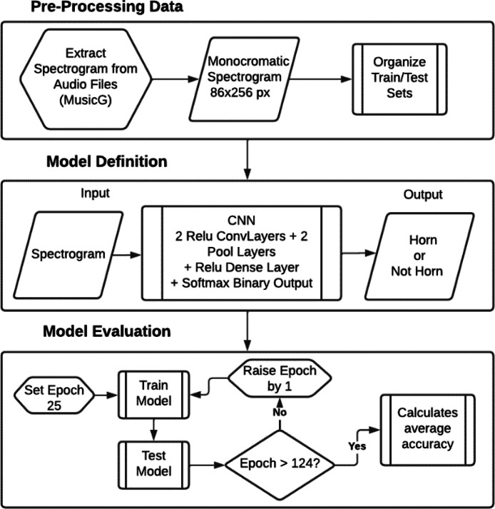
Convolutional Neural Networks (CNNs) have established themselves in the literature as a powerful tool for image classification and are demonstrating increasing success in sound classification tasks. They outperform traditional algorithms like Support Vector Machines (SVMs) and Gaussian Mixture Models (GMMs) [14]. Because of that, a CNN model was chosen to analyze the HornBase Dataset. Spectrograms in grayscale format with dimensions of 86×256 pixels were extracted from the audio files using the MusicG [15] library in Java. Then, the CNN architecture was defined and 100 models were trained using TensorFlow [16] in Python. Fig. 4 provides a visual overview of the entire process. In the following subsections, each step of the presented pipeline will be detailed.

Fig. 4.

Dataset evaluation pipeline.

5.1. Spectrogram Extraction with MusicG

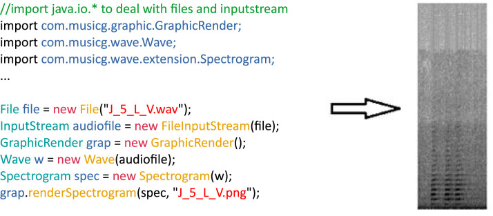
The MusicG library written in Java was used to extract spectrograms from the audio files in the dataset. MusicG can read .wav files and generate grayscale spectrograms, among other functionalities. Algorithm 1 shows a code snippet demonstrating how to import the necessary classes, read an audio file, and generate the spectrogram plot.

Algorithm 1.

Code Snippet for extracting a spectrogram with MusicG.

The provided example demonstrates spectrogram generation for a single audio file. The generated spectrogram is essentially a heat map where the most prominent frequency regions in the 1-second window of the audio are darker, with lower frequencies at the bottom of the image, and higher frequencies at the top.

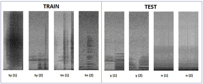
In order to handle the large dataset efficiently, the Windows PowerShell tool was used to rename the files to a pattern suitable for iterative processing in loops. For instance, the training set files were renamed following the pattern ty (1), ty (2) ... ty (m) for positive class, and tn (1), tn (2) ... tn (m) for negative class. The same logic was applied to the test set, renaming files to y (1), y (2) ... y (m) and n (1), n (2) ... n (m) for positive and negative classes, respectively. Note that positive class indicates the occurrence of a horn, and negative class indicates its absence. A demonstration of the generated spectrograms, with the files in this nomenclature, is presented in Fig. 5.

Fig. 5.

Sample of the spectrograms for each set and class.

After separating the training and testing sets and renaming the files, we proceeded to load the spectrograms into Python using the OpenCV library [17] for grayscale reading, as illustrated in Algorithm 2.

Algorithm 2.

Loading Spectrograms with OpenCV in Python

5.2. Model Definition and Evaluation

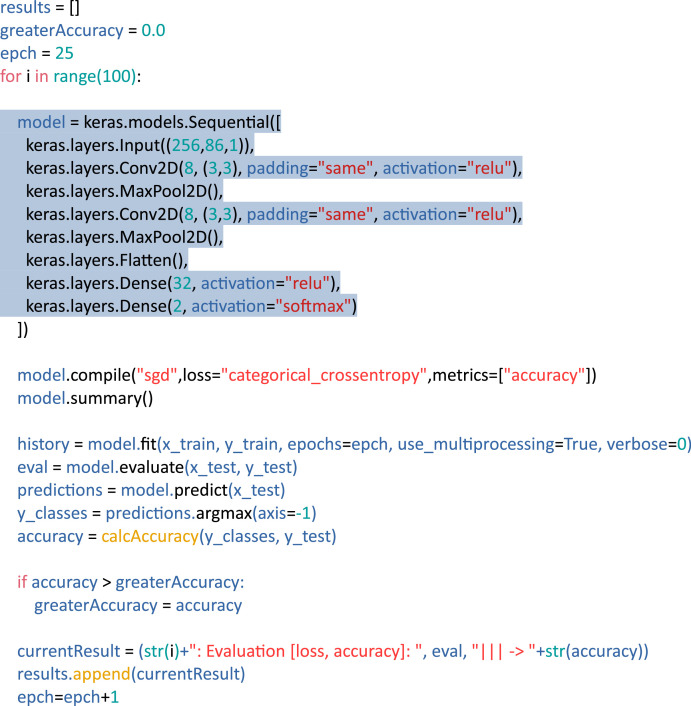
A basic CNN architecture was designed, consisting of an input layer that accepts the entire spectrogram image. It was followed by a convolutional layer with a 3×3 kernel and a ReLU (Rectified Linear Unit) activation function. A pooling layer was then applied for dimensionality reduction. We stacked another convolutional layer with a 3×3 kernel, ReLU activation, and another pooling layer to extract more complex features. The resulting feature map was flattened into a one-dimensional vector, which was fed into a fully-connected layer with ReLU activation. Finally, the output layer used a Softmax activation function to provide binary class probabilities.

The training was parameterized with variable epochs. For an initial test, we arbitrarily set the epochs to 100, and the model achieved an accuracy of 95%, as detailed in Table 3. However, a closer look at the confusion matrix (vide Table 2) reveals that most errors were false negatives. In other words, the model did not identify some horn samples, prompting further investigation with different approaches.

Table 3.

Measures from confusion matrix.

Measure	Value
Accuracy	0.959
Recall	0.938
Precision	0.980
F1 Score	0.959

Table 2.

Confusion matrix.

	True Positive	True Negative
Predicted Positive	152	3
Predicted Negative	10	159

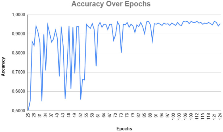
In order to verify if the accuracy of the model in this specific training was not merely coincidental, a sequence of 100 models were trained, with epochs ranging from 25 to 124, incrementing by one for each subsequent training. Consequently, the models exhibited an overall average accuracy of 89%, as illustrated by the evolution curve in Fig. 6. Notably, there is significant fluctuation in accuracy between epochs 25 and 90, followed by a period of minor oscillation thereafter.

Fig. 6.

Evolution of accuracy over epochs.

The Python code developed to architect the CNN, conduct the training in a loop of 100 models, and generate the test results for each iteration can be viewed in Algorithm 3, where the highlighted excerpt reveals the CNN architecture itself.

Algorithm 3.

Implementation of 100 CNNs in Python.

Our exploration using the HornBase Dataset involved feature extraction (spectrograms), training a basic CNN model, and evaluation. This process achieved an average accuracy of 89%. These results indicate that the proposed protocol for creating the audio dataset is viable, and HornBase can be a valuable resource for horn detection model pipelines.

Considering future work, we recommend investigating the extraction of additional features suitable for different machine learning models. Additionally, the action of exploring more robust CNN architectures can broaden the scope of evaluation and potentially improve accuracy. All codes presented in this paper are publicly available at https://github.com/cleytondim/HornBase.

Limitations

Due to concerns about the safety of individuals involved in audio collection and other drivers, as well as to avoid potential traffic violations by continuously honking, the route taken was planned on a low-traffic street. Consequently, it lacks sounds from environments with heavier traffic.

Due to resource limitations, we focused on constructing the dataset exclusively with car horns. This strategic decision emphasizes the significance of capturing and understanding the nuances of car horn sounds in various scenarios. Acknowledging the absence of horns sounds from other vehicles, we recommend using the developed database in applications that aim to reproduce the real world, but keeping in mind the predominance of cars.

Some other potential scenarios were considered, such as rain, thunder, and sirens in the external environment, but due to their occurrences being challenging to predict at a specific time in the real world, they were discarded.

Ethics Statement

The authors have read and follow the ethical requirements for publication in Data in Brief. The production of the data collected did not involve any human subjects, animal experimentation. It is self-produced and doesn't have any data from social media platforms.

CRediT Author Statement

Cleyton Aparecido Dim: Conceptualization, Validation, Investigation, Methodology, Software, Data Curation, Writing - Original Draft. Nelson Cruz Sampaio Neto: Conceptualization, Formal analysis, Supervision, Writing - Review & Editing. Jefferson Magalhães de Morais: Conceptualization, Methodology, Formal analysis, Supervision, Writing - Review & Editing.

Data Availability

• HornBase - A Car Horns Dataset (Original data) (Mendeley Data).

References

- 1.Saba M.M.F., Rosa R.A.S. The Doppler effect of a sound source moving in a circle. Phys. Teach. 2003;41(2):89–91. [Google Scholar]
- 2.Dim C.A., Feitosa R.M., Mota M.P., Morais J.M. Computational Science and Its Applications – ICCSA 2020. Springer; 2020. A smartphone application for car horn detection to assist hearing-impaired people in driving. Lecture Notes in Computer Science, vol. 12250. [DOI] [Google Scholar]
- 3.Dim C.A., Feitosa R.M., Mota M.P., Morais J.M. Alert systems to hearing-impaired people: a systematic review. Multimed. Tools Appl. 2022;81:32351–32370. doi: 10.1007/s11042-022-13045-1. [DOI] [Google Scholar]
- 4.Salamon J., Jacoby C., Bello J.P. Proceedings of the 22nd ACM international conference on Multimedia (MM '14) Association for Computing Machinery; New York, NY, USA: 2014. A dataset and taxonomy for urban sound research; pp. 1041–1044. [DOI] [Google Scholar]
- 5.Piczak K.J. Proceedings of the ACM International Conference on Multimedia. ACM; 2015. ESC: dataset for environmental sound classification; pp. 1015–1018. [Google Scholar]
- 6.Fonseca E., Favory X., Pons J., Font F., Serra X. vol. 30. 2022. FSD50K: an open dataset of human-labeled sound events; pp. 829–852. (IEEE/ACM Transactions on Audio, Speech, and Language Processing). [DOI] [Google Scholar]
- 7.Foster P., Sigtia S., Krstulovic S., et al. 2015 IEEE Workshop on Applications of Signal Processing to Audio and Acoustics (WASPAA) IEEE; 2015. CHiME-home: a dataset for sound source recognition in a domestic environment. [Google Scholar]
- 8.Kabealo R., Wyatt S., Aravamudan A., et al. A multi-firearm, multi-orientation audio dataset of gunshots. Data Brief. 2023;48 doi: 10.1016/j.dib.2023.109091. [DOI] [PMC free article] [PubMed] [Google Scholar]
- 9.Estacio R.S.P., Montenegro D.A.B., Rodas C.F.R. Dataset of audio signals from brushless DC motors for predictive maintenance. Data Brief. 2023;50 doi: 10.1016/j.dib.2023.109569. [DOI] [PMC free article] [PubMed] [Google Scholar]
- 10.Becker S., Vielhaben J., Ackermann M., et al. AudioMNIST: exploring explainable artificial intelligence for audio analysis on a simple benchmark. J. Franklin. Inst. 2024;361:418–428. doi: 10.1016/j.jfranklin.2023.11.038. [DOI] [Google Scholar]
- 11.Tomasello P., Shrivastava A., Lazar D., et al. IEEE Spoken Language Technology Workshop (SLT) 2022. Stop: a dataset for spoken task oriented semantic parsing; pp. 991–998. [DOI] [Google Scholar]
- 12.Nigro M., Krishnan S. SARdB: a dataset for audio scene source counting and analysis. Appl. Acoust. 2021;178 doi: 10.1016/j.apacoust.2021.107985. [DOI] [Google Scholar]
- 13.Bhogale K., Raman A., Javed T., et al. IEEE International Conference on Acoustics, Speech and Signal Processing (ICASSP) 2023. Effectiveness of mining audio and text pairs from public data for improving ASR systems for low-resource languages; pp. 1–5. [DOI] [Google Scholar]
- 14.Su Y., Zhang K., Wang J., Madani K. Environment sound classification using a two-stream CNN based on decision-level fusion. Sensors. 2019;19(7):1733. doi: 10.3390/s19071733. [DOI] [PMC free article] [PubMed] [Google Scholar]
- 15.Musicg. MusicG - lightweight java API for audio analysing, android compatible. In: https://code.google.com/archive/p/musicg, accessed in Apr 10 2024.
- 16.TensorFlow. An end-to-end platform for machine learning. In: https://www.tensorflow.org/, accessed in Apr 20 2024.
- 17.OpenCV. Open computer vision library. In: https://opencv.org/, accessed in Apr 25 2024.
Associated Data
This section collects any data citations, data availability statements, or supplementary materials included in this article.
Data Availability Statement