Real-time tracking of structural evolution in 2D MXenes using theory-enhanced machine learning

Abstract

In situ Electron Energy Loss Spectroscopy (EELS) combined with Transmission Electron Microscopy (TEM) has traditionally been pivotal for understanding how material processing choices affect local structure and composition. However, the ability to monitor and respond to ultrafast transient changes, now achievable with EELS and TEM, necessitates innovative analytical frameworks. Here, we introduce a machine learning (ML) framework tailored for the real-time assessment and characterization of in operando EELS Spectrum Images (EELS-SI). We focus on 2D MXenes as the sample material system, specifically targeting the understanding and control of their atomic-scale structural transformations that critically influence their electronic and optical properties. This approach requires fewer labeled training data points than typical deep learning classification methods. By integrating computationally generated structures of MXenes and experimental datasets into a unified latent space using Variational Autoencoders (VAE) in a unique training method, our framework accurately predicts structural evolutions at latencies pertinent to closed-loop processing within the TEM. This study presents a critical advancement in enabling automated, on-the-fly synthesis and characterization, significantly enhancing capabilities for materials discovery and the precision engineering of functional materials at the atomic scale.

Introduction

Two-dimensional (2D) functional materials, such as MXenes and other transitional metal-based inorganic systems, are at the forefront of materials development for improving electrodes for energy storage¹, next-generation semiconductors for electronics², and magneto-optics for data storage³. The unique capabilities of these carbide, nitride, and carbonitride systems are driving a revolution in these fields. Yet, to fully exploit these materials, it is crucial to gain a more precise understanding of their chemical coordination and electronic structure, which are intimately linked to their composition and specific material properties^4,5. The ability to manipulate surface terminations in MXenes opens up new avenues to tune both physical and chemical properties, presenting opportunities to tailor these materials for specific applications. Control over these surface terminations is pivotal as they directly influence the material's reactivity, conductivity, and overall stability, making them a key focus for targeted material engineering^5,6. However, most characterization and discussion of termination is completed at the bulk scale using methods such as vibrational spectroscopy, nuclear magnetic resonance spectroscopy^7,8, thermogravimetric-differential scanning calorimetry^9,10, and electron dispersive spectroscopy (EDS) in the scanning electron microscopy (SEM)^11,12, These methods, while useful, often fall short of providing the necessary resolution to fully resolve the atomic-scale subtleties crucial for optimizing material performance. To address this gap, higher-resolution techniques are essential. Techniques like scanning probe microscopy¹³, atom probe tomography¹⁴, and transmission electron microscopy (TEM)^15,16 offer the spatial resolution required to probe the local structures of these complex systems effectively. Such detailed analysis is critical for advancing our understanding of 2D materials and harnessing their full potential, enabling the design of more efficient, high-performance materials tailored to meet the rigorous demands of modern technological applications.

TEM offers exceptional spatial resolution, providing an information-rich characterization of material structure and local configuration. More specifically, probing electronic structure through Scanning Transmission Electron Microscopy—Electron Energy Loss Spectroscopy (STEM-EELS) reveals bonding information at or below the 1 Å level. This capability is essential for understanding the intricate details of atomic arrangements and electronic interactions that define the functionality of 2D materials. By enabling precise characterization at such a fine scale, STEM-EELS emerges as a powerful tool for directly observing and analyzing the fundamental properties that influence material performance at the atomic level^17,18. STEM-EELS’s ultra-high spatial resolution, combined with significant advances in sensing technologies, such as direct detection systems^19,20, enables high rates of data collection, more than 400 spectra per second and improved signal fidelity, the ability to count electrons instead of relative intensities for indirect detection systems. While direct detection systems greatly increase the signal-to-noise ratio (SNR)²¹, the rate of data collection and the size of the total dataset created²², an approach for qualitatively and quantitatively uncovering changes in the near-edge structure, has not evolved to the same extent. Current methods rely on measuring height ratio changes, energy shifts, and relative intensities to extrapolate changes in the electronic structure in the sample²³. This includes comparison to both labeled experimental datapoints and computationally simulated near-edge structure. With the advent of machine learning (ML), we now have access to a powerful tool for pattern recognition and distilling trends from microscopy and spectroscopy datasets^24–29. Exploiting the power of ML tools for this purpose will be the focus of this paper.

The ability to employ ML frameworks for a rapid classification of local chemical structure on 2D functional materials would not only greatly improve our understanding of the surface functionalization of these systems but would also allow for feedback control to be added to the TEM instrument. If it were possible to embed decision-making with informed classification into the TEM, we would be able to do more than simply probe atomic structure, it would also open the door to engineering precise surface chemistries intended to maximize material performance^30,31. For these aspirations to become a reality, the requisite decision framework will need to include rapid feature extraction, classification against possible chemical configurations, and the ability to extract sufficient signal from noisy spectra with few-electron events. Recent studies have demonstrated different approaches to some of these capabilities, although not all^25,32,33. In contrast, this study outlines a framework that is uniquely suited for providing rapid feature embedding and classification and enabling direct feedback control and decision for operando techniques such as electron beam control or heating control for engineering materials within the TEM autonomously.

There has certainly been a lot of ML tool-based activity in this area. Feature extraction, denoising, and background subtraction via ML have been explored in different approaches for hyperspectral datasets: Approaches include matrix factorization techniques such as principal component analysis (PCA), non-negative matrix factorization (NMF)^24,27,34, and other statistical methods as well as various “deep learning” models such as autoencoders^25,35,36, convolutional neural networks²⁸, and other tensor-based methods. Statistical methods have been incredibly powerful in denoising capabilities with PCA approaches, including tools which are incorporated directly with tools such as Digital Micrograph^26,37,38 and Hyperspy³⁹. Matrix factorization has also been a proven method for deconvolution of overlapping edges to map SIs²⁴ and extracting distinct spectral features for improved spatial mapping of compounds^27,34. Deep learning approaches are similarly good performers in denoising and classification of spectral data. Approaches such as random forest^33,40 and CNN offer high classification accuracy, but necessitate large, labeled datasets^28,29. Autoencoder approaches, including variational autoencoders (VAEs) have demonstrated both denoising³⁵ and the creation of non-linear feature embedding for clustering and classification²⁵. The dimensionality reduction in VAEs differs from matrix factorization methods due to the non-linear nature⁴¹ and the ability to decouple more significant factors without dataset bias unlike PCA and similar methods⁴². Most importantly, the latent embeddings from VAEs have been demonstrated to relate multiple features across different inputs, such as relating STEM imaging to spectral data³⁶, or spectral features to structural descriptors^25,32.

Despite this activity, the classification methods described above share a common challenge in the reliance on extensive, labeled training data. By this we mean the use of datasets of any modality in which the structure or bond interactions are known and classified for each datapoint. This can be done through a traditional analysis by a human or by using computational means to generate simulated datasets wherein the structure calculation is known. The former is not feasible in many cases, and the latter can be prohibitively computationally expensive. Human generated labels is the main approach for most supervised learning approaches but requires large amounts of time from a domain expert to create a dataset. To offset bias from the scientist making the labels, multiple results from different domain experts should be combined and resolved. For spectroscopic datasets such as EELS, it is common that not all structures present nor potential intermediates are known, and these methods are designed for classifying only known labels. Additionally, the number of datapoints for these transient states may not be significant enough to form distinct clusters in unsupervised methods, as demonstrated in the previous study on SrFeO₃³⁵. For a closed loop framework to classify operando experiments, it cannot rely on the availability of large, labeled datasets, computationally or experimentally generated, and needs to provide a robust unsupervised feature extraction capable of isolating and classifying chemical configurations. This is the challenge our paper seeks to address.

In this paper, we demonstrate a variational dual autoencoder framework designed for embedding theory for the classification of highly spatiotemporal localized STEM-EELS datasets, focusing on 2D MXenes. This framework, described in Fig. 1, provides the basis for precise feedback loops and control in future autonomous studies involving these advanced materials. The unsupervised encoder model effectively embeds both low signal-to-noise ratio (SNR) single-pixel spectra and computationally simulated “fingerprint” spectra into the same latent feature representation. These fingerprint spectra, particularly representative of 2D MXenes' unique surface terminations, serve as the basis for classification across different structural compositions. By resolving the clustering behavior of experimental data distribution against the feature space based on computationally modeled structures of MXenes, the model is capable of estimating classification and uncertainty in a semi-supervised approach. The result is a rapid classification of noisy single spatio-temporal pixels against a library of a few simulated structures. Implementing this framework into the analysis process allows the model to evaluate structural changes, resolved spatially and temporally against simulated structures directly from EELS-SI. This approach removes the need for large labeled experimental or theoretical datasets in addition to providing an unsupervised, non-linear latent space with informed distributions of simulated structures.

Figure 1.

Workflow diagram of the variational autoencoder, shown as three major steps: (1) experimental data are used to train unsupervised feature extraction, (2) computational data are used for classification and cluster analysis, (3) resulting denoised signals and classification mapping.

Results

To demonstrate the framework discussed above, an in situ EELS-SI dataset was used consisting of three scan areas of Cr₂TiC₂O_xF_y annealed up to 800° C. The full dataset includes 24 EELS-SI consisting of 570 individual spectra, each measured at a wide dispersion in order to include Ti L_2,3, O K, Cr L_2,3, and F K edges within the measured window. This experimental dataset was previously discussed in Hart et al.^15,43 but the SNR on single-pixel spectra was too low to resolve any spatial relevant changes to the near-edge structure. This necessitates the use of machine learning to probe both spatial and temporal accuracy of the ‘as collected’ dataset without the need to integrate along either axis.

Four edges are captured within the energy window, the Ti L_2,3, O K, Cr L_2,3, and F K edges. Cr₂TiC₂O_xF_y, akin to other 2D MXenes, features characteristic surface functional groups (-O, -F). At elevated temperatures, these functional groups begin to decompose while the core structure comprising carbon, chromium, and titanium is generally stable. Among these, fluorine is notably more volatile and less thermally stable than oxygen group and starts to dissociate from the material. This dissociation of fluorine is a significant transformation during annealing, prominently reflected in changes to the F K-edge, as shown in Fig. 2. As fluorine leaves the structure, there is a reduction in electron-withdrawing effects that fluorine typically imposes on the metal atoms in MXenes. This change in surface chemistry can modify the electronic structure, potentially enhancing electrical conductivity and altering electrochemical properties by increasing free carrier concentrations or modifying the band structure⁴⁴. Therefore, characterizing surface terminations is essential for understanding their functionalities. In terms of spectral analysis, the relationship between the first peak height of the F K-edge and the annealing temperature is particularly telling. Isolating this shoulder-peak ratio returns a characteristic functionalization quantification that can be used to indicate changes across the entire dataset. If no shoulder remains, but a peak still exists, this will indicate no remaining fluorine terminations. The remaining peak is the result of the Cr L₁-edge and aluminum fluoride, which was noted in a previous study¹⁵. These structural changes, present in the experimental datasets, are supported by simulated spectra based on computed structures for various chemical configurations. These compositions were chosen based on the EXELFS (Extended Energy Loss Fine Structure) analysis in a prior study using the Cr K-edge for this material system⁴³. Multiple configurations were simulated for each composition based on density functional theory (DFT) structure calculations performed at different ratios of F:O.

Figure 2.

Spatially averaged spectra for a set of annealing temperatures from initial room temperature (25 °C) to 700 °C, as indicated on the inset as experimental (“EXP”) data. Corresponding simulated spectra derived from DFT-generated structures shown as solid lines as denoted in the inset as “CALC” (DFT-generated) curves for different ratios of F:O, ranging from 1.1 to 1.7, as indicated. The cosine similarities between the simulated data and the experimental data are all above 0.95.

The temporal temperature series demonstrates a conventional analysis wherein spatial information is lost in favor of increasing the SNR. Averaging across the spatial axis increases the signal as demonstrated in Fig. 3a–d, indicates that it is extremely important to average the signal over multiple pixels (here shown up to 32-pixel averaging). In stark contrast, ML methods, including PCA and deep learning approaches, are powerful approaches for extracting signal, even at the individual pixel level, increasing the spatio-temporal resolution to match the maximum rate of the detector of 400 frames per second¹⁹. Figure 3e,f illustrates this capability, where the SNR of the PCA and VAE de-noised single-pixel spectra area comparable to the spatially averaged spectra. This demonstrates that ML-generated means can act as an effective alternative to averaging datapoints across spatial or temporal axes in order to increase signal above the noise variation intensity.

Figure 3.

Intensity as a function of energy loss for: (a–d) single pixel (a), a few pixels (8- and 16- in (b) and (c)), versus many (32-) pixel averages for the dataset (d). Images (e,f) denote single pixel results as denoised by PCA (e) and VAE (f) approaches. Color indicates the temperature ranges for each spectra collected and averaged, indicating how the peak changes with temperature can be visualized with increased signal over noise.

Single-pixel spectra are used to train a modified variational autoencoder, creating a latent space fitted to a normal distribution “prior.” The training data used consists of the original single pixel spectra seen in Fig. 3a, and the PCA denoised spectra seen in Fig. 3e. The VAE is trained to encode and decode the PCA spectra while a secondary encoder is trained on the raw single pixel spectra. This dual encoder structure is fit to a convergence loss between the latent space of the raw encoder and PCA trained encoder. This allows for raw, noisy datapoints to be embedded into the same latent feature space and be denoised via the decoder, shown in Fig. 3f.

The simulated spectra are then fed into the PCA-trained encoder, giving a mean and log-variance as the “fingerprint” for each computationally derived structure. Sampling this mean and log-variance with a random normal density function creates a distribution for each composition which acts as the classification label. The distribution generated from the encoder is learned from the experimental dataset in the unsupervised training dataset, and decoding these latent distributions illustrates how these learned features are represented in the original near-edge spectra. An example of this process is shown in Fig. 4 with sample distributions for two of the VAE latent dimensions chosen to emphasize the separation of each composition in the feature embeddings. The generated latent space datapoints serve as the training data for the latent space semi-supervised classifier. This classifier takes the 16-dimensional feature embeddings, from either encoder, as an input and outputs a class corresponding to one of the compositions present in the computationally generated spectra. Applying this trained classifier to the experimental embeddings results from the raw encoder in direct label classification for single-pixel results. The final framework structure consists of the raw spectra-encoder performing feature extraction and a classifier model performing an inference based on the latent space inputs.

Figure 4.

Workflow to illustrate the creation of a labeled latent distribution of the dataset based on DFT-generated structure calculations (left) with feature extraction from the encoder trained originally on experimental data (middle), producing decoder-generated spectra (right).

A Gaussian process classifier was found to perform well for this use-case. An additional advantage of this classifier is the ability to extract probabilities for identifying datapoints with high uncertainty in prediction. Applying the trained classifier to the latent embeddings of the experimental data generates a classification which can be constructed into a full STEM map, wherein each pixel of the spectrum image, consisting of a single raw spectrum, is transformed into a composition label. This approach mirrors a traditional elemental quantification map that can be generated via STEM-EELS wherein, instead of elemental edge intensities, the color is directly correlated with calculated structures. The results can be seen in Fig. 5, as produced by the semi-supervised classifier run on the latent encodings of single pixel data (top row). This is compared with a classification map generated by denoising each spectrum via PCA (bottom row) and assigning an estimated composition label based on the relative peak and shoulder heights, as indicated in Fig. 2.

Figure 5.

STEM classification as produced from both the VAE semi-supervised approach (top row) and peak-shoulder ratio measurements on PCA-denoised results (bottom row) across each annealing temperature studied (from RT to 800 C). This classification shows the decrease in fluorine content with increasing temperature. The PCA approach erroneously shows a rich fluorine region at high temperatures, in contrast to the VAE approach. Color key as indicated.

As shown in Fig. 5, the classification results for both the VAE and PCA approaches readily identify reduction in fluorine content as the temperature increases. This effect dominates at 600°C, denoted by the color change from predominantly yellow (50% F) to predominantly blue (12.5% F) for PCA results, and from yellow to green (25% F) using the VAE approach. This supports previous studies^15,43 on this dataset identifying the change in near-edge structure of the F K-edge at high temperatures and the reduction in fluorine nearest neighbor peaks in the Cr K-edge extended fine structure. The two approaches thus differ greatly in classifications at high annealing temperatures. A major difference occurs in the 600°C map (right side, STEM-EELS map, Fig. 5) where the PCA maps result in high fluorine content compared to the VAE results that indicate a far less striking reduction in F content. At lower annealing temperatures, this same region is low in fluorine, evident in both approaches. The variance in low temperature classification maps is higher in PCA.

Classification maps illustrate the trends in structure changes with temperature; but further analysis of the denoised EELS spectra will be needed to fully evaluate the changes present in the dataset. Figure 6 shows denoised signals produced by PCA and VAE approaches. Notably, the VAE-denoised signal depicts significant changes in the annealed spectra with minimal to no fluorine content compared to the PCA-denoised approach. The residual shoulder in the PCA data indicates a statistical bias present in the data; the annealed spectra are known (from a previous study)¹⁵ to produce a single peak. Importantly, the pre-peak standard deviations are considerably higher in the PCA-denoised results compared to the VAE-denoised ones. This comparison shows that the VAE approach is much better equipped to extract non-linear features of the near-edge structure signatures, which is further supported by Fig. 7a, comparing the feature space embeddings. By comparing the dimensionality reduced space, reduced to two dimensions via t-distributed stochastic neighbor embeddings (t-SNE)⁴⁵, it is evident how structural changes present in the dataset are directly related to extracted features in the latent space representations of the VAE. The separation of features in the latent space representation directly relates to the ability of the model to discern real changes in the data versus noise. PCA is still capable of extracting trends in the dataset, as evident by the gradient of labels across the embedding axes, but the clustering capabilities in the VAE produce more cohesive regions of each structure class. This comparison indicates that the VAE performs better in identifying features in the dataset that are directly related to structural changes This is further supported by the silhouette score in Fig. 7b indicating that, for each increase in the temperature series, the VAE outperforms the PCA approach.

Figure 6.

Denoised F K-edge spectra via VAE (left) and PCA (right) approaches shown as solid lines, with corresponding means (solid lines) and standard deviations (lightly shaded regions) for each classification label based on the inputted computationally generated spectra. Color key given below the curves for different amounts of fluorine from 50% (yellow) to 0% (purple).

Figure 7.

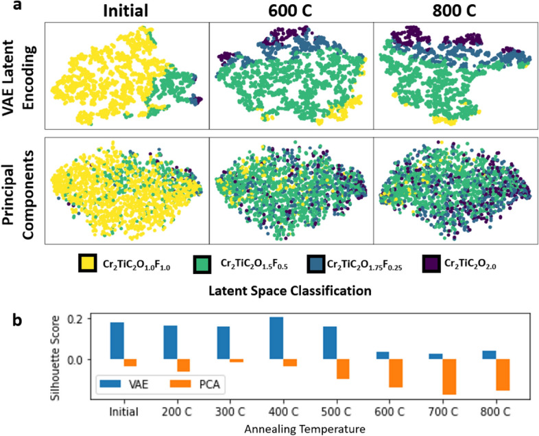
(a) t-Stochastic Neighbor Embedding (t-SNE) plots for both VAE latent encodings and principal components, demonstrating how feature extraction of the latent encodings is more directly related to structural features present in the EELS dataset compared to PCA. This is supported quantitatively by the silhouette score (b), which is a measure of clustering performance given by the spatial distance of ‘like’ datapoints compared to ‘unlike’ datapoints.

Since real-time inference is a requirement for using the demonstrated framework as a part of a feedback loop, runtime performance of the model needs to be minimized. Runtime for the encoder structure within a Jupyter Notebook was measured for a single 32 spectra batch at 54 ms ± 5.2 ms using the default Tensorflow⁴⁶ runtime with GPU acceleration. This does not include the time taken to preprocess the data or load into memory. Compiling the TensorFlow model into a TensorRT⁴⁷ engine gives a performance improvement to 0.209 ms ± 0.0015 ms.

Discussion

This study demonstrates the capabilities of variational autoencoders in decoding structural changes within EELS datasets and correlating these latent variances to computationally generated structures. While this VAE framework does not replace the need for thorough ex situ comparison and detailed quantitative analysis, it represents a significant advancement by offering rapid classification and informed latent feature embedding, particularly in analyzing near-edge structural changes observed in EELS data. Specifically, in our study, this approach allows for real-time tracking of surface termination changes during the annealing process and provides insights into corresponding shifts in electrochemical properties of MXenes. This development is a critically important first step toward "intelligent microscopy," where automated, precise adjustments enhance the understanding and manipulation of material properties at the microscopic level.

The requirements set out for enabling intelligent microscopy were as follows: rapid extraction of relevant chemical features, classification against possible chemical configurations, and inference on low SNR datasets. Unlike existing solutions, this framework does not rely on large, comprehensive, labeled ground truth data for classifier training. Instead, it relies only on the availability of a few hand-picked structure calculations for the basis of classification. This differs from other dominant methods such as convolutional neural networks (CNNs) or random forest models, which rely on training data consisting of each potential class label. Additionally, this framework differs from other unsupervised clustering algorithms as it introduces a means to establish a basis for classification within the model framework without a “human in the loop” interpretation of clusters. Relying on human labeling of classification data for training machine learning models is a major bottleneck in the development of new models and a large source of error and uncertainty in models. Finally, the ability to perform inference on noisy single pixel datapoints is on par with the denoising performance of popular, accepted methods such as PCA, but the VAE latent representation outperforms the dimensionality reduced feature space of principal components in its ability to extract features, which directly corresponds to structural changes present in the EELS dataset.

In addition to the performance improvements in feature extraction provided by the VAE framework, an important novel contribution is the direct relationship of structural changes to the latent embeddings output from the encoder. Principal components are capable of identifying statistical changes present inside the STEM-EELS dataset. However, the VAE encoder structure does not just identify those trends with high accuracy, reinforced by the silhouette score, but also relates structural changes to distinct clusters within the latent space distribution. An example of this ability is illustrated in Fig. 4 where the embedded computationally generated structures are used as the underlying classification basis for the experimental data. This is an important distinction when applying the framework towards autonomous experimentation. The latent features correlated with structural fingerprints paired with classification labels provide the uncertainty quantification necessary for decision-making frameworks required for intelligent microscopy.

Several challenges are still present in this study and will need to be addressed going forward. Pushing the limit on spatio-temporal resolution of EELS results in difficulty of identifying valid ground truth labels for validation of classification results. Previous studies have relied on integration of multiple spatial or time points within the dataset to provide a basis for validating the machine learning results. However, if variation across each axis is high, this results in dilution of sparsely represented features, which can result in ground truths that are not representative of the original dataset. For the MXene annealing data presented in this study, the best available ground truth comes from spatially averaged or single-pixel PCA-denoised results. For validating a framework targeted at moving beyond those limitations, a reporting accuracy based upon the aforementioned ground truths would not be representative.

The framework presented here offers a necessary first step towards enabling engineered functional materials to be created with atomic precision. This framework is focused on exploring the chemical space present within STEM-EELS data and doing so with high spatial and temporal precision. This ability to extract signal from small volumes and time steps in a method that can be automated will provide the foundation for building real-time feedback loops into the TEM. Estimating candidate structures in real-time shifts the microscope from a characterization tool into a processing tool, capable of targeting local structure with the precision of the convergent electron beam. Using classification maps with precision electron patterning toolsets⁴⁸, inducing structural changes in response to local real-time classification will enable precision engineering of materials. Before such methods can be employed, however, there are several additional steps, beyond what we have achieved here, that will need to be implemented. For example, paired with any classification estimate, an uncertainty quantity should be included to provide context to further models regarding the error and extrapolation from the VAE framework. Two sources of uncertainty are propagated into each prediction, from the latent encoding and from the classification method. Any decision framework utilizing inference from this framework will need to weight inferences based on the paired uncertainty. Additionally, including this uncertainty component will aid in active learning methods such as Bayesian frameworks⁴⁹, critical for exploratory closed-loop methods.

Furthermore, the present simulation results rely on the availability of pristine crystal structures, which will not account for defects that could arise during the annealing process. Unfortunately, due to the complexity of structural changes and the number of possible defective configurations, structures with defects were not considered for the training dataset in this work. Encouraged by the success of our introduction of non-terminated surface sites into the system, the use of refined (more realistic) structures can enhance the agreement between simulation and experiments, and thus further improve the accuracy of the classification. By combining DFT calculations for structures that include defects, along with the uncertainty evaluation and active learning techniques mentioned earlier, we can effectively and efficiently identify actual structures without the need to construct an extensive DFT dataset in a high-throughput manner. Ultimately, this approach paves the way for the realization of automated, on-the-fly synthesis and characterization—an exciting prospect that could elevate material design to the next level.

Methods

Model structure

The framework consists of a variational autoencoder (VAE) trained to extract features from high SNR experimental data, and a secondary standard encoder used to relate the low SNR data to the same latent feature space. The VAE for unsupervised feature-extraction is based on the previous RapidEELS autoencoder framework³⁵ where 1D convolutional layers are stacked, with a single dense layer performing the last bottleneck step. This model improves considerably on the previous work by incorporating a VAE structure, by the addition of a secondary encoder, and by the incorporation of computational fingerprints as a basis of classification. Unlike traditional autoencoder frameworks, VAEs utilize a Kullback–Leibler (KL)⁵⁰ divergence factor to fit the latent variables to a probability distribution such as a Gaussian Normal^41,51. The main variational encoder-decoder pair is trained to process high SNR experimental data such as spatially averaged, time-integrated, or PCA-denoised data to build out the feature embeddings. The secondary encoder is given a loss function related to the difference between the latent outputs of low SNR encoder and the latent mean outputs from the high SNR encoder for a given raw and denoised training datapoint. This is called the “convergence loss” and is the sum of the absolute error between the latent outputs of each encoders. Through this structure, both noisy, single pixel datapoints and high SNR-denoised or simulated EELS spectra can be related in a single, continuous latent feature space.

The additional capability of this structure is the ability to use the variational encoder to return a distribution of latent embeddings sampled from the mean and log-variance outputs. This distribution is directly related to the learned structure from the experimental dataset used to train the VAE in an unsupervised manner. By doing so, it is possible to generate a labeled dataset based on computed structures for training a supervised clustering algorithm without the need for running many different variations of structure calculations and simulating near-edge structure spectra for each.

Model setup and training

As discussed in Pate et al.³⁵, the mean absolute error is used for the reconstruction loss as it is more resistant to outliers than the mean squared error. The reason PCA-denoised data is used in place of spectra summed over an area is due to spatial changes in the spectra across the collection area. This variance is due to heterogeneity in the sample thickness more than functionalization changes at a given condition and hence gives rise to noise in the analysis.

TensorFlow 2.11.0⁴⁶ and the Keras API was used to construct and train the encoder, decoder and neural network classifier models. Batch and layer normalization were avoided due to consistent tendency for overfitting the datasets. A test-train split of 10% to 90% was used for training the VAE as a method of validating whether new data can be embedded into the latent space without falling out of domain.

Latency measurements and compiling

The latency measurements were performed on an NVIDIA RTX 2060 Max-Q. The compiled engine was produced using the TensorRT toolkits provided by NVIDIA to optimize the model for the hardware⁴⁷. The measurements were averaged from ten runs of inferences performed on a single batch of size 32. The compiled engine was limited to 16-bit floating point calculations while the native TensorFlow model performed inference at 32-bit floating point precision. Only the encoder portion of the model was measured since this would be the portion used for decision making in a real-time closed loop system.

Latent space classification

The feature embeddings extracted from the dataset in the VAE latent space are trained through unsupervised means. Unsupervised clustering algorithms can be employed at this point to pair similar features into groupings based on the dimensionally reduced space. Instead, this study employed a supervised classification algorithm trained on the latent space features generated from the simulated spectra. The labels directly correspond to chemical compositions used as the basis for the structure calculations. We tested several classification algorithms but the Gaussian process classifier⁵², as implemented in Sci-Kit Learn⁵³, was chosen due to ability to perform an inference between the encoded experimental data and the encoded computationally generated data. The latent space distribution plots were generated by performing a t-stochastic neighbor embedding (t-SNE) on the latent dimensions output from the encoder. This provided a means of visualizing the 16-dimensional latent features to a two-component value for visualization. PCA initialization was used for both the latent outputs and the PCA outputs for the t-SNE plots.

Since low-latency is a primary focus of the framework, an additional classifier can be included by constructing a dense neural classifier and appending this to the experimental encoder. This method was introduced in the previous study³⁵ for classification and consists of a few dense layers applied at the end of the encoder layers. This is trained using the same latent space dataset generated from the simulated dataset. This effectively forms a convolutional neural network consisting of the encoder paired with the dense classifier which has the advantage of being accelerated using edge compute devices such as Field Programmable Gate Arrays⁵⁴. This is unlike the algorithmic based classification used in the Gaussian process classifier. The result is a reduction in the overall framework latency at the expense of a small trade-off in accuracy.

In situ electron spectroscopy

The EELS Spectrum Images used for this study were collected using a JEOL 2100F (Schottky Field Emission Source), equipped with a Gatan Imaging Filter and a K2 Summit Direct Detection Sensor. Pixel size was about 13 nm with an exposure time of about 0.1s at an energy dispersion of 0.125 eV per channel. The MXene samples were deposited onto a DENSsolutions Lightning D9 + sample holder for heating and biasing Eight different conditions were measured, including the initial condition, at each of seven temperatures up to 800°C in increments of 100°C. Data used for this study were previously published in Hart et al.¹⁵ and this study serves to add additional context to the spatial component of the experiment through the aid of machine learning. Additional information on sample preparation and microscope configuration can be found in the Methods section and in the Supplemental Information.

Dataset processing

The EELS dataset was imported from Gatan DM4 files as Spectrum Images, using Hyperspy’s Python API³⁹. No spatial information from the dataset is passed into the autoencoder, only individual spectra. The dataset consisted of 13,680 individual spectra. These datapoints were collected from eight, 19 × 30 spectrum images (570 spectra) at each of the different temperatures mentioned in the in situ methods section. For the input dataset, spectra were rebinned, from a 0.125 eV energy dispersion to 0.25 eV-per channel, in order to more closely match the measured energy resolution of the electron source. Additional pre-processing aligned all spectra in the energy axis to the Cr-L2 and Cr-L3 edges, and normalized intensities of the same peaks. A set window of 677 to 737 eV was extracted in order to capture the F K-edge. A power-law fit for background subtraction was used to isolate the F K-edge from the background. No deconvolution was performed with the zero-loss SI since only the high-loss signal was collected at each temperature and using the zero-loss peak from before heating would not account for any thickness changes occurred throughout the annealing process. If present, the deconvolutions would better normalize datapoints compared to the area under the curve method. Dual EELS mode, collecting the zero-loss and high-loss signals simultaneously is not feasible on the K2 Summit due to the small sensor size. The presence of the zero-loss peak would also provide a more accurate energy shift correction, such as the zero-loss peak lock provided natively in most EELS collection software. The analysis was performed on both the ‘as collected’ spectrum images, as well as a PCA-denoised dataset generated by a Digital Micrograph²⁶ using 10 principal components.

Simulating EELS spectra

Plane-wave periodic density functional theory (DFT) calculations for the MXene structures, including the lattice constants and atomic positions, were carried out using QUANTUM ESPRESSO⁵⁵. The simulation workflow is illustrated in Fig. 8. PBEsol⁵⁶ was chosen as the exchange–correlation functional, as it was found to reproduce the experimental formation enthalpy adequately⁵⁷. The convergence criteria were set at 1 × 10^–8 eV for total energy per unit cell and 0.01 eV/Å for forces. The plane-wave cutoff energy was set at 550 eV and a k-point grid of 10 × 10 × 1 was chosen according to the convergence tests (within 0.01 eV/atom). The two surface layers contained eight atoms in total to enable modeling of the surface-termination changes during the annealing process. A vacuum region of 15 Å was used on both surface layers. Specifically, we considered full O termination (O:F = 8:0) and three mixed terminations (O:F = 7:1, 6:2 and 4:4). For each composition, we constructed all possible configurations and only the stable (energy preferred) ones were used for subsequent spectra calculations. The final configurations of different compositions are shown in the Supplemental Information.

Figure 8.

Simulation workflow: (a) Step 1: Calculate possible configurations for a user-supplied composition. Two example stable structures are shown for a relaxed MXene with a fluorine-to-oxygen ratio, F:O of 3:5. (b) Step 2: Calculate spectra for each stable structure and obtain a representative ensemble average (here four structures were used). (c) Step 3: Comparison with experimental results and fine-tuning of broadening parameters, if needed.

Core-loss spectra calculations were carried out using Finite Difference Method Near Edge Structure (FDMNES)⁵⁸. We recognize that FDMNES is designed for XAS calculations rather than for EELS. The key difference between these two lies in the double-differential cross-section_. When the absorption energy is far above 100 eV, as in the case of the F K-edge investigated in this work, this difference becomes trivial⁵⁹. Therefore, in this study, we use FDMNES to approximate EELS. We compared the predicted spectra based on DFT calculations to those from time-dependent DFT (TDDFT); the differences between the resulting spectra are inconsequential. Quadrupolar components and relativism effects were also considered. Based on the convergence test evaluated by cosine similarity and Pearson correlation (0.99), the cluster radius was set as 6 Å and the cell size was set as 2 × 2. For each composition (at different ratios between fluorine and oxygen), the spectra were calculated from the site-averaged O/F-K edge of all energy preferred configurations. In total, we have eight simulated spectra as the training data.

Author contributions

J.D.H., C.M.P., and M.L.T. devised the concept of the machine learning framework; M.L.T. led the program; J.D.H. and M.L.T. formed the ideation for the final implementation; J.D.H., C.M.P., H.J., J.L.H., P.C., M.L.T. discussed the approach for integrating the machine learning with simulations; J.D.H., C.M.P. designed the machine learning framework; J.D.H. built and trained the model and performed the statistical analysis; H.J. designed, optimized, and evaluated the computationally generated structures and simulated spectroscopy; J.L.H. performed the microscopy experiment and analytical analysis; J.D.H., H.J. created the figures; J.D.H., H.J. wrote the manuscript with support from P.C. and M.L.T.; All authors reviewed the manuscript.

Data availability

Access to the full EELS dataset is available upon request to the corresponding author. The pre-processed is provided in the Github repository for this project. Python code for this study can be found at https://github.com/hollejd1/logicalEELS containing the autoencoder framework, and notebooks for training the model and replicating the figures.

Competing interests

The authors declare no competing interests.

Supplementary Information

The online version contains supplementary material available at 10.1038/s41598-024-66902-4.

References

- 1.Anasori, B., Lukatskaya, M. R. & Gogotsi, Y. 2D metal carbides and nitrides (MXenes) for energy storage. Nat. Rev. Mater.2(2), 1–17 (2017). 10.1038/natrevmats.2016.98 [DOI] [Google Scholar]
- 2.Choi, W. et al. Recent development of two-dimensional transition metal dichalcogenides and their applications. Mater. Today20, 116–130 (2017). 10.1016/j.mattod.2016.10.002 [DOI] [Google Scholar]
- 3.Li, Y. et al. Insights into electronic and magnetic properties of MXenes: From a fundamental perspective. Sustain. Mater. Technol.34, e00516 (2022). [Google Scholar]
- 4.Su, T. et al. Surface engineering of MXenes for energy and environmental applications. J. Mater. Chem. A Mater.10, 10265–10296 (2022). 10.1039/D2TA01140A [DOI] [Google Scholar]
- 5.Yang, Q., Eder, S. J., Martini, A. & Grützmacher, P. G. Effect of surface termination on the balance between friction and failure of Ti3C2Tx MXenes. NPJ Mater. Degrad.7(1), 1–8 (2023). 10.1038/s41529-023-00326-9 [DOI] [Google Scholar]
- 6.Gholivand, H., Fuladi, S., Hemmat, Z., Salehi-Khojin, A. & Khalili-Araghi, F. Effect of surface termination on the lattice thermal conductivity of monolayer Ti3C2Tz MXenes. J. Appl. Phys.126, 65101 (2019). 10.1063/1.5094294 [DOI] [Google Scholar]
- 7.Harris, K. J., Bugnet, M., Naguib, M., Barsoum, M. W. & Goward, G. R. Direct measurement of surface termination groups and their connectivity in the 2D MXene V2CTx using NMR spectroscopy. J. Phys. Chem. C119, 13713–13720 (2015). 10.1021/acs.jpcc.5b03038 [DOI] [Google Scholar]
- 8.Björk, J. & Rosen, J. Functionalizing MXenes by tailoring surface terminations in different chemical environments. Chem. Mater.33, 9108–9118 (2021). 10.1021/acs.chemmater.1c01264 [DOI] [Google Scholar]
- 9.Li, J. et al. Achieving high pseudocapacitance of 2D titanium carbide (MXene) by cation intercalation and surface modification. Adv. Energy Mater.7, 1602725 (2017). 10.1002/aenm.201602725 [DOI] [Google Scholar]
- 10.Han, K., Zhang, X., Deng, P., Jiao, Q. & Chu, E. Study of the thermal catalysis decomposition of ammonium perchlorate-based molecular perovskite with titanium carbide MXene. Vacuum180, 109572 (2020). 10.1016/j.vacuum.2020.109572 [DOI] [Google Scholar]
- 11.Arif, N., Gul, S., Sohail, M., Rizwan, S. & Iqbal, M. Synthesis and characterization of layered Nb2C MXene/ZnS nanocomposites for highly selective electrochemical sensing of dopamine. Ceram. Int.47, 2388–2396 (2021). 10.1016/j.ceramint.2020.09.081 [DOI] [Google Scholar]
- 12.Shahzad, A. et al. Two-dimensional Ti3C2Tx MXene nanosheets for efficient copper removal from water. ACS Sustain. Chem. Eng.5, 11481–11488 (2017). 10.1021/acssuschemeng.7b02695 [DOI] [Google Scholar]
- 13.Sahare, S. et al. An assessment of MXenes through scanning probe microscopy. Small Methods6, 2101599 (2022). 10.1002/smtd.202101599 [DOI] [PubMed] [Google Scholar]
- 14.Krämer, M. et al. Near-atomic scale perspective on the oxidation of Ti3C2Tx MXenes: insights from atom probe tomography. Adv. Mater.10.1002/adma.202305183 (2023). 10.1002/adma.202305183 [DOI] [PubMed] [Google Scholar]
- 15.Hart, J. L. et al. Control of MXenes’ electronic properties through termination and intercalation. Nat. Commun.10(1), 1–10 (2019). 10.1038/s41467-018-08169-8 [DOI] [PMC free article] [PubMed] [Google Scholar]
- 16.Persson, I. et al. How much oxygen can a MXene surface take before it breaks?. Adv. Funct. Mater.30, 1909005 (2020). 10.1002/adfm.201909005 [DOI] [Google Scholar]
- 17.Wang, Z. et al. In situ STEM-EELS observation of nanoscale interfacial phenomena in all-solid-state batteries. Nano Lett.16, 3760–3767 (2016). 10.1021/acs.nanolett.6b01119 [DOI] [PubMed] [Google Scholar]
- 18.Goodge, B. H., Baek, D. J. & Kourkoutis, L. F. Atomic-resolution elemental mapping at cryogenic temperatures enabled by direct electron detection (2020).
- 19.Hart, J. L. et al. Direct detection electron energy-loss spectroscopy: A method to push the limits of resolution and sensitivity. Sci. Rep.7(1), 1–14 (2017). 10.1038/s41598-017-07709-4 [DOI] [PMC free article] [PubMed] [Google Scholar]
- 20.Tate, M. W. et al. High dynamic range pixel array detector for scanning transmission electron microscopy. Microsc. Microanal.22, 237–249 (2016). 10.1017/S1431927615015664 [DOI] [PubMed] [Google Scholar]
- 21.Maigné, A. & Wolf, M. Low-dose electron energy-loss spectroscopy using electron counting direct detectors. Microscopy67, i86–i97 (2018). 10.1093/jmicro/dfx088 [DOI] [PubMed] [Google Scholar]
- 22.Spurgeon, S. R. et al. Towards data-driven next-generation transmission electron microscopy. Nat. Mater.20(3), 274–279 (2020). 10.1038/s41563-020-00833-z [DOI] [PMC free article] [PubMed] [Google Scholar]
- 23.Williams, D. B. & Carter, C. B. Transmission electron microscopy: A textbook for materials science 1–760 (2009) 10.1007/978-0-387-76501-3/COVER.
- 24.Jia, H., Wang, C., Wang, C. & Clancy, P. Machine learning approach to enable spectral imaging analysis for particularly complex nanomaterial systems. ACS Nano17, 453–460 (2023). 10.1021/acsnano.2c08884 [DOI] [PubMed] [Google Scholar]
- 25.Ziatdinov, M., Ghosh, A., Wong, C. Y. & Kalinin, S. V. AtomAI framework for deep learning analysis of image and spectroscopy data in electron and scanning probe microscopy. Nat. Mach. Intell.4(12), 1101–1112 (2022). 10.1038/s42256-022-00555-8 [DOI] [Google Scholar]
- 26.MSA for DigitalMicrograph—HREM Research Inc. https://www.hremresearch.com/msa/.
- 27.Ryu, J. et al. Dimensionality reduction and unsupervised clustering for EELS-SI. Ultramicroscopy231, 113314 (2021). 10.1016/j.ultramic.2021.113314 [DOI] [PubMed] [Google Scholar]
- 28.Timoshenko, J., Lu, D., Lin, Y. & Frenkel, A. I. Supervised machine-learning-based determination of three-dimensional structure of metallic nanoparticles. J. Phys. Chem. Lett.8, 5091–5098 (2017). 10.1021/acs.jpclett.7b02364 [DOI] [PubMed] [Google Scholar]
- 29.Mizoguchi, T. & Kiyohara, S. Machine learning approaches for ELNES/XANES. Microscopy69, 92–109 (2020). 10.1093/jmicro/dfz109 [DOI] [PubMed] [Google Scholar]
- 30.Peng, J., Chen, X., Ong, W.-J., Zhao, X. & Li, N. Surface and heterointerface engineering of 2D MXenes and their nanocomposites: Insights into electro- and photocatalysis. (2019) 10.1016/j.chempr.2018.08.037.
- 31.Najam, T. et al. Synthesis and nano-engineering of MXenes for energy conversion and storage applications: Recent advances and perspectives. Coord. Chem. Rev.454, 214339 (2022). 10.1016/j.ccr.2021.214339 [DOI] [Google Scholar]
- 32.Tetef, S., Govind, N. & Seidler, G. T. Unsupervised machine learning for unbiased chemical classification in X-ray absorption spectroscopy and X-ray emission spectroscopy. Phys. Chem. Chem. Phys.23, 23586–23601 (2021). 10.1039/D1CP02903G [DOI] [PubMed] [Google Scholar]
- 33.Gleason, S. P., Lu, D. & Ciston, J. Prediction of the Cu oxidation state from EELS and XAS spectra using supervised machine learning. (2023).
- 34.Shiga, M. et al. Sparse modeling of EELS and EDX spectral imaging data by nonnegative matrix factorization. Ultramicroscopy170, 43–59 (2016). 10.1016/j.ultramic.2016.08.006 [DOI] [PubMed] [Google Scholar]
- 35.Pate, C. M., Hart, J. L. & Taheri, M. L. RapidEELS: Machine learning for denoising and classification in rapid acquisition electron energy loss spectroscopy. Scientific Reports11(1), 1–10 (2021). 10.1038/s41598-021-97668-8 [DOI] [PMC free article] [PubMed] [Google Scholar]
- 36.Roccapriore, K. M. et al. Predictability of localized plasmonic responses in nanoparticle assemblies. Small17, 2100181 (2021). 10.1002/smll.202100181 [DOI] [PubMed] [Google Scholar]
- 37.Watanabe, M., Kanno, M., Ackland, D., Kiely, C. & Williams, D. Applications of electron energy-loss spectrometry and energy filtering in an aberration-corrected JEM-2200FS STEM/TEM. Microsc. Microanal.13, 1264–1265 (2007). 10.1017/S1431927607079184 [DOI] [Google Scholar]
- 38.Gatan Microscopy Suite Software|Gatan, Inc. https://www.gatan.com/products/tem-analysis/gatan-microscopy-suite-software.
- 39.Peña, F. de la et al. Hyperspy/hyperspy: Release v1.7.3. (2022) 10.5281/ZENODO.7263263
- 40.Zheng, C., Chen, C., Chen, Y. & Ong, S. P. Random forest models for accurate identification of coordination environments from X-ray absorption near-edge structure. Patterns1, 100013 (2020). 10.1016/j.patter.2020.100013 [DOI] [PMC free article] [PubMed] [Google Scholar]
- 41.Ruineihart, D.E., Hint, G.E. & Williams, R.J. Learning internal representations berror propagation two. (1985).
- 42.Lichtert, S. & Verbeeck, J. Statistical consequences of applying a PCA noise filter on EELS spectrum images. Ultramicroscopy125, 35–42 (2013). 10.1016/j.ultramic.2012.10.001 [DOI] [PubMed] [Google Scholar]
- 43.Hart, J. L. et al. Multimodal spectroscopic study of surface termination evolution in Cr2TiC2Tx MXene. Adv. Mater. Interfaces8, 2001789 (2021). 10.1002/admi.202001789 [DOI] [Google Scholar]
- 44.Papadopoulou, K. A., Chroneos, A., Parfitt, D. & Christopoulos, S. R. G. A perspective on MXenes: Their synthesis, properties, and recent applications. J. Appl. Phys.128, 170902 (2020). 10.1063/5.0021485 [DOI] [Google Scholar]
- 45.Van Der Maaten, L. & Hinton, G. Visualizing data using t-SNE. J. Mach. Learn. Res.9, 2579–2605 (2008). [Google Scholar]
- 46.Developers, T. TensorFlow. 10.5281/ZENODO.7604226 (2022). 10.5281/ZENODO.7604226 [DOI]
- 47.NVIDIA Corporation. TensorRT SDK. Preprint at https://github.com/NVIDIA/TensorRT (2024).
- 48.Reed, B. W. et al. Electrostatic switching for spatiotemporal dose control in a transmission electron microscope. Microsc. Microanal.28, 2230–2231 (2022). 10.1017/S1431927622008595 [DOI] [Google Scholar]
- 49.Mukherjee, D. et al. A roadmap for edge computing enabled automated multidimensional transmission electron microscopy. Micros Today30, 10–19 (2022). 10.1017/S1551929522001286 [DOI] [Google Scholar]
- 50.Kullback, S. & Leibler, R. A. On Information and Sufficiency10.1214/aoms/117772969422 (1951). 10.1214/aoms/117772969422 [DOI] [Google Scholar]
- 51.Kingma, D. P. & Welling, M. Auto-Encoding Variational Bayes. 2nd International Conference on Learning Representations, ICLR 2014 - Conference Track Proceedings (2013).
- 52.Rasmussen, C. E. & Williams, C. K. I. Gaussian Processes for Machine Learning.
- 53.Pedregosa Fabianpedregosa, F. et al. Scikit-learn: Machine learning in Python. J. Mach. Learn. Res.12, 2825–2830 (2011). [Google Scholar]
- 54.Castellana, V. G. et al. Towards on-chip learning for low latency reasoning with end-to-end synthesis. Proceedings of the Asia and South Pacific Design Automation Conference, ASP-DAC 632–638 (2023) 10.1145/3566097.3568360.
- 55.Giannozzi, P. et al. QUANTUM ESPRESSO: A modular and open-source software project for quantum simulations of materials. J. Phys.: Condens. Matter21, 395502 (2009). [DOI] [PubMed] [Google Scholar]
- 56.Perdew, J. P. et al. Restoring the density-gradient expansion for exchange in solids and surfaces. Phys. Rev. Lett.100, 136406 (2008). 10.1103/PhysRevLett.100.136406 [DOI] [PubMed] [Google Scholar]
- 57.Ibragimova, R., Puska, M. J. & Komsa, H. P. PH-dependent distribution of functional groups on titanium-based MXenes. ACS Nano13, 9171–9181 (2019). 10.1021/acsnano.9b03511 [DOI] [PMC free article] [PubMed] [Google Scholar]
- 58.Bunǎu, O. & Joly, Y. Self-consistent aspects of X-ray absorption calculations. J. Phys.: Condens. Matter21, 345501 (2009). [DOI] [PubMed] [Google Scholar]
- 59.Mauchamp, V., Boucher, F., Ouvrard, G. & Moreau, P. Ab initio simulation of the electron energy-loss near-edge structures at the Li K edge in Li, Li2O, and LiMn2O4. Phys. Rev. B74, 115106 (2006). 10.1103/PhysRevB.74.115106 [DOI] [Google Scholar]
Associated Data
This section collects any data citations, data availability statements, or supplementary materials included in this article.
Data Citations
- Developers, T. TensorFlow. 10.5281/ZENODO.7604226 (2022). 10.5281/ZENODO.7604226 [DOI]
Supplementary Materials
Data Availability Statement