Abstract
As Europe integrates more renewable energy resources, notably offshore wind power, into its super meshed grid, the demand for reliable long-distance High Voltage Direct Current (HVDC) transmission systems has surged. This paper addresses the intricacies of HVDC systems built upon Modular Multi-Level Converters (MMCs), especially concerning the rapid rise of DC fault currents. We propose a novel fault identification and classification for DC transmission lines only by employing Long Short-Term Memory (LSTM) networks integrated with Discrete Wavelet Transform (DWT) for feature extraction. Our LSTM-based algorithm operates effectively under challenging environmental conditions, ensuring high fault resistance detection. A unique three-level relay system with multiple time windows (1 ms, 1.5 ms, and 2 ms) ensures accurate fault detection over large distances. Bayesian Optimization is employed for hyperparameter tuning, streamlining the model’s training process. The study shows that our proposed framework exhibits 100% resilience against external faults and disturbances, achieving an average recognition accuracy rate of 99.04% in diverse testing scenarios. Unlike traditional schemes that rely on multiple manual thresholds, our approach utilizes a single intelligently tuned model to detect faults up to 480 ohms, enhancing the efficiency and robustness of DC grid protection.
Keywords: High voltage direct current (HVDC), Long short-term-memory (LSTM), Primary protection, DC circuit breaker (DCCB), Discrete wavelet transform (DWT)
Subject terms: Energy science and technology, Engineering, Electrical and electronic engineering, Energy infrastructure
Introduction
In recent years, the extensive adoption of renewable power generation in European nations has underscored the need for robust transmission systems1. High voltage direct current (HVDC) transmission, renowned for efficiently transmitting power over long distances, emerges as a pivotal technology2. HVDC systems offer a practical solution for harnessing wind power from offshore stations to onshore locations. Offshore wind energy transmission to onshore grid stations requires a viable infrastructure using submarine cables and overhead lines, ensuring efficient and reliable transmission. However, the efficacy of such transmission systems, especially those spanning long distances and encountering complex environmental factors, hinges on addressing the high probability of line failures. In the context of mixed lines in transmission systems, achieving precise and prompt fault location becomes imperative. This prerequisite for enhancing the overall reliability of power systems becomes even more critical considering the challenges posed by long-distance transmission and the intricacies introduced by natural environmental factors.
For the practical realization of a future multi-terminal (MT-HVDC) grid, a promising candidate is the HVDC grid built upon the modular multi-level converter (MMC)3. However, integrating multiple converters introduces challenges, notably the rapid rise of DC fault currents due to low inertia4,5. Managing these high DC fault currents and protecting power electronic devices become critical considerations. Extremely quick DC fault detection systems that can locate faults in 2–4 ms are desperately needed to control high DC fault currents5. This urgency underscores the importance of diagnosing fault transients with a high-speed operational perception and efficiently isolating them to safeguard the integrity of the power transmission system.
In literature, various transient-based methods have emerged for HVDC grid protection, with a central focus on feature extraction and classification. Feature extraction aims to capture data characteristics in subordinate dimensions within the time, frequency, or frequency-time domain. Commonly used signal processing tools include Fourier transform (FT) or wavelet transform (WT) for discerning signal variations6,7. These variations are computed using straightforward processing approaches that consider the signal’s rate of change variations, amplitude-based shifts, or statistical principles like wavelet entropy, wavelet energy, and spectrum distribution8,9. After signal processing, specific features are extracted to facilitate fault protection.
In contrast, many DC fault protection methods in the literature rely on thresholding, and a few leverages artificial intelligence (AI). Typically, fault classification involves logical relationships with thresholds10,11. However, the widespread use of multiple manual thresholds can compromise the robustness of the protection scheme12. The challenges are exacerbated by the non-periodic nature and significant fluctuations of fast DC fault transients under dynamic operational conditions, necessitating a more robust approach for quick fault detection.
AI-based fault classification presents a flexible approach for addressing non-linear systems, offering solutions under complex selection criteria and overcoming challenges associated with manual thresholds13. AI algorithms, including support vector machines (SVM) and backpropagation neural networks (BP-NN)14,15, have found applications in HVDC protection. For instance, the protection of the MMC-HVDC system involved using thirteen artificial neural network (ANN) models16, achieving high model accuracy at the expense of increased computational burdens. A convolutional neural network (CNN) was proposed for a two-terminal MMC-HVDC system17. However, the impact of noise and its applicability to the DC grid were not discussed. While researchers employ AI-based techniques for DC grid protection18,19, these methods introduce challenges. The utilization of traditional deep neural networks (DNN) in MMC fault diagnostics faces difficulties in extracting fault features that vary over time due to the unextendible time dimension20. This limitation can be addressed by employing a long-short-term memory (LSTM) model.
The LSTM model exhibits a unique feature learning ability, allowing it to derive information from the current feedback and stored information at the previous moment. This capability enables LSTM to overcome shortcomings in traditional DNN, especially in MMC fault diagnosis21. Serving as an advanced version of recurrent neural networks (RNN)22, LSTM’s superior structural variation has found applications across various domains, excelling in text classification, speed recognition, and other areas23,24.
Considering the dynamic operational conditions of HVDC systems, conventional Neural Network (NN) techniques exhibit deficiencies in DC grid protection, including complex calculations, inaccuracy, vulnerability to electrical noises, less robustness, and reliance on expensive signal processing tools. We propose a DC fault classification approach leveraging the LSTM algorithm to address these limitations. Previous studies25 emphasize the pivotal role of fault identification in non-linear systems, acknowledging that LSTM, like traditional NNs, is susceptible to overfitting and mis-convergence in the face of non-linearity. Strategies such as incorporating dropout layers and adjusting hyperparameters are implemented to mitigate these challenges. Hyperparameter optimization is crucial for enhancing neural network efficiency and overcoming the issues mentioned earlier. While previous studies often rely on trial-and-error methods for hyperparameter selection26, our approach utilizes Bayesian Optimization (BO) to streamline the optimization process and ensure the specification of parameters governing NN structure and model training.
The proposed algorithm integrates the discrete wavelet transform (DWT) for feature extraction, enhancing the robustness of its output27,28. This approach contributes significantly to the engineering framework for MMC-HVDC systems, effectively bridging the gap between theoretical concepts and practical data-driven intelligent relay design. The main contributions of this study are:
The main aim of this study is to detect and classify DC transmission line faults by observing DC signals, whereas not generate any false trip signal due to external faults such as AC fault.
We propose a novel fault identification and classification approach employing Long Short-Term Memory (LSTM) networks integrated with Discrete Wavelet Transform (DWT) for feature extraction. This integration enhances the robustness of the model, particularly in the presence of noise and high fault resistance conditions.
Three-level relays with multiple time windows (1 ms, 1.5 ms, and 2 ms) allow for accurate fault detection over long distances without backups. With this innovative approach, the LSTM network can be mapped and trained over a 200 km distance, resulting in accurate fault detection.
Unlike traditional protection schemes relying on multiple manual thresholds obtained through worst-case studies, the proposed algorithm streamlines the process using a single intelligently tuned BO model. This contributes to a more efficient and robust fault classification approach.
While double-sided protection is conventionally preferred due to global positioning systems, the proposed scheme eliminates the need for communication links between MMC stations. In addition to reducing signal interference and delays during the protection process, this innovation enhances system reliability by providing faster response, reduced maintenance costs, and compatibility with existing infrastructure.
The subsequent sections of this paper are structured as follows: "MT-HVDC test bench" introduces the MT-HVDC test bench. "Feature extraction" elaborates on the feature extraction methodology implemented in the study. "Long-term short-term memory" discusses the architecture of LSTM networks. "implementation of the proposed algorithm" details the implementation of the proposed algorithm, followed by “Proposed protection scheme”, which presents the proposed protection scheme. "Evaluation of the proposed protection mechanism" evaluates the efficacy of this scheme. Finally, “Conclusions and future research directions” concludes the study.
MT-HVDC test bench
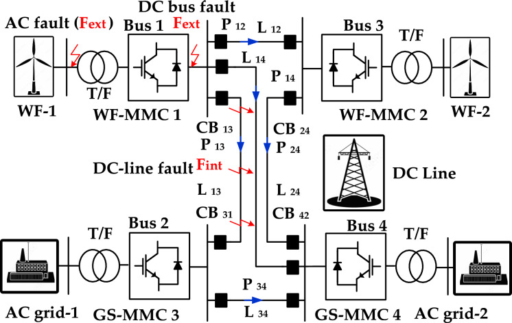
A meshed four-terminal MMC-HVDC test bench, as depicted in Fig. 1, has been implemented in PSCAD/EMTDC to investigate various fault scenarios. Internal faults within the DC transmission line, labelled as Fint, include negative-pole-to-ground (N-PTG), positive-pole-to-ground (P-PTG), and pole-to-pole (PTP) faults29,30. External faults outside the DC-line boundary are denoted as Fext. The symmetrical monopole test bench consists of two offshore MMC terminals supplying electrical power to two onshore MMC terminals with voltage droop control. DC overhead lines are used to evaluate high-power transmission systems. A 10 mH smoothing inductor is connected to both ends of the transmission lines to suppress high fault currents. The DC-link voltage is rated at ± 320 kV. Lastly, Hybrid-DCCB is attached at each end of the DC link for fault current interruption, as specified in31. Table 1 provides the parameters of the controller, DC, and AC systems. The transient characteristics of DC fault signals are rigorously studied using the frequency-dependent phase model.
Figure 1.
Schematics of four-terminal MMC-HVDC test bench with DC overhead lines.
Table 1.
Main parameters of four-terminal HVDC test bench.
| Station | Nominal voltage (kV) | Arm inductance/mH | Capacity/MW | SM capacitance/mF | DC system | Length (km) |
|---|---|---|---|---|---|---|
| MMC-1 | ± 320.0 | 84.80 | 3000.0 | 15.0 | OHL-12 | 100 |
| MMC-2 | 84.80 | 2000.0 | 10.0 | OHL-13 | 200 | |
| MMC-3 | 84.80 | 2500.0 | 12.50 | OHL-14 | 200 | |
| MMC-4 | 63.60 | 1500.0 | 8.0 | OHL-34 | 200 |
Feature extraction
In the HVDC grid, distinct features in current and voltage signals during pre- and post-fault scenarios play a crucial role in detecting internal and external faults. Analyzing these signals is essential for extracting unique features, typically achieved through signal processing tools. However, capturing transient signal information that lasts only a few milliseconds presents a significant challenge. Our study employs the second norm of DWT to accurately extract fast-decaying and high-frequency transient features from voltage signals to address this. DWT offers time- and frequency-dominance localization, whereas CWT is continuous32.
Feature extraction utilizing discrete wavelet transform
The use of the DWT is a strategic choice in our study due to its superior speed, accuracy, efficient selectivity, and heightened resolution in handling transient signals. This transformative approach enables a detailed and efficient analysis of transient signals, significantly enhancing the precision of DC fault detection. DWT, in comparison to the Fourier transform (FT), offers distinct advantages, and its mathematical definition is articulated as32:
| 1 |
The parameters ‘n’ and ‘m’ in this context are integers, playing crucial roles in the translation and dilation of the mother wavelet, signifying sampling number and decomposition level, respectively. corresponds to the mother wavelet. Multi-resolution analysis (MRA) is used after DWT as a first step in signal decomposition. The method allows the signal to be segregated into distinct scales, enabling the extraction of distinct fault characteristics from the input signals, as illustrated in Fig. 2.
Figure 2.
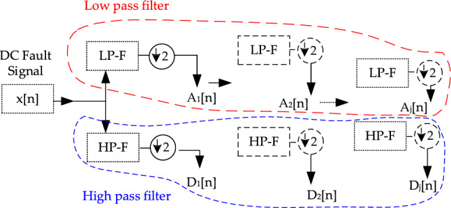
Multi-resolution fault signal decomposition until the nth level.
For a fault signal, x(t), the process of multi-resolution signal decomposition requires both scaling and wavelet functions to assess fault condition specifics within the framework of the DWT. This assessment is expressed as follows:
| 2 |
| 3 |
| 4 |
where and are conjugates of the scaling function and wavelet function , respectively. k is an integer variable corresponding to a sample number in an input signal. J is the maximum number of decomposition levels. As an example, the original signal can be represented as follows using 4-scale decomposition:
| 5 |
As part of the MRA method, high-pass, and low-pass filters are used to decompose the signal into approximate (representing low-frequency-components) and detail coefficients (representing high-frequency components). For DC transient faults in HVDC grids to be accurately classified, it is essential to have a precise representation of the transformed signal. Therefore, the following subsection examines input features for DC fault studies.
Analysis of input features
The DC fault protection system’s startup criteria are designed to activate protective measures when abnormal fault current conditions are detected. A predefined current threshold, denoted as Tthreshold, is established to achieve this. This threshold is higher than the system’s standard operating current and is determined based on system specifications, fault scenarios, and safety margins.
| 6 |
The startup condition is defined as follows: if the absolute value of the measured DC fault current, represented as Ifault, exceeds the predefined threshold, the startup criteria are met as in (7):
| 7 |
A hysteresis band is introduced around the threshold level to prevent rapid startup and shutdown due to minor current fluctuations that may occur. Specifically, a hysteresis value, denoted as H, is applied. The startup criteria are considered met once the absolute value of the fault current exceeds Ithreshold + H or falls below Ithreshold − H. This hysteresis band stabilizes the startup decision, as expressed in (8) and (9).
| 8 |
| 9 |
Transient current spikes may cause false startup triggers. A time delay mechanism is therefore implemented to avoid any false startups. The startup condition must persist for a defined duration, denoted as Tdelay, before initiating protective actions. During this time, continuous monitoring confirms the fault condition as given by (10):
| 10 |
A startup signal is generated once the startup criteria are met and confirmed. This signal activates the broader DC fault protection system, including protective relays and fault isolation measures, ensuring a timely response to potential faults. Additionally, communication mechanisms are in place to transmit the startup signal promptly to the control center responsible for managing the protection system. Periodic self-testing is implemented to verify the integrity of the startup criteria and sensors. Any fault or malfunction within the startup criteria detected during self-testing triggers a maintenance alert. Integrating the startup criteria seamlessly with the overall DC fault protection relay system, ensuring effective coordination with other protective measures for the system’s safety and stability.
Upon initializing the startup parameters, a methodology for extracting features from the input signal is meticulously developed. The algorithm’s input feature extraction assumes that high-frequency elements in the DC-line voltage behave differently under internal faults. This behavior is attributed to the influence of current-limiting inductors at varying fault locations. As demonstrated in Fig. 3, the transient variations in the DC-line voltage under an internal fault scenario rise more sharply than those triggered by external faults. A subsequent frequency analysis, also represented in Fig. 4, reveals that these high-frequency elements are less prominent in external fault situations. Therefore, this information segment serves as a critical tool for differentiating faults that originate within the system from those that are externally induced33.
Figure 3.
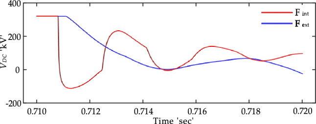
The slope of VDC under external (DC-bus) and internal fault.
Figure 4.
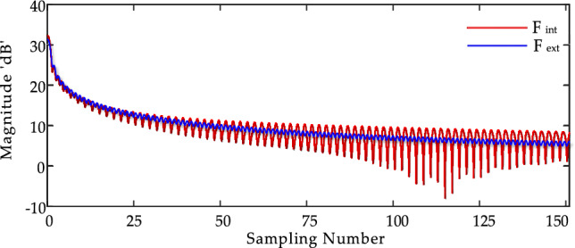
VDC frequency spectrum under external (DC-bus) and internal fault.
Upon closer inspection of internal faults, precisely PTP faults, it becomes clear that both the positive (VP) and negative (VN) pole voltages experience similar variations. Conversely, during a PTG fault, the voltage alteration varies significantly between the two poles, as illustrated in Figs. 5 and 6.
Figure 5.
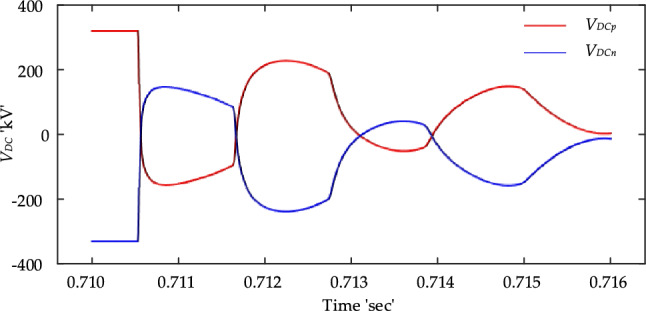
VDC variation under PTP fault.
Figure 6.
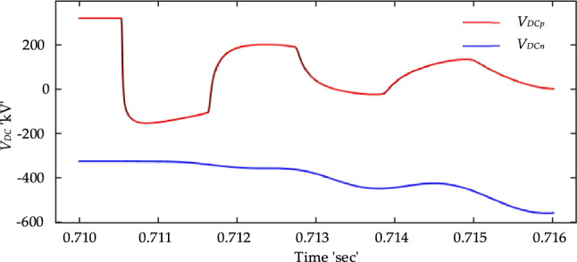
VDC variation under PTG fault.
Changes in the voltage of the affected pole also influence the voltage of the unaffected pole, owing to the interconnected nature of the negative and positive DC lines. A phase-modal transformation is employed to separate and analyze the voltages of both poles into distinct lines and zero modes to address these changes in the voltages. In the event of a positive-to-ground (P-PTG) fault, the absolute variations in the DC-line voltage at both the negative and positive poles, denoted as ∆VN and ∆VP, can be measured by the relationship given in (11) and (12):
| 11 |
| 12 |
In this context, Bl0 and Bl1 represent the impedances for zero-sequence and positive-sequence pathways, extending from the fault point to the local terminal. ‘U’ denotes half the standard voltage between the poles, and Bg signifies the impedance encountered at the fault location. The proportional change between the unaffected and affected pole voltages consistently adheres to the relationship in (13):
| 13 |
As a result, the sum of Bl0 and Bl1 exceeds their difference, leading to a consistently smaller value for ∆VN compared to ∆VP. On the other hand, in the case of a N-PTG fault, ∆VN exceeds ∆VP. These observations establish that the variations in VDC (DC voltage), in conjunction with fluctuations in ∆VN and ∆VP, serve as useful criteria for distinguishing between normal and faulted conditions in DC transmission lines.
Selection of features
As mentioned earlier, we construct our proposed regression model by incorporating the second norm of wavelet coefficients. This is done after analyzing the input features consisting of VDC, ∆VN, and ∆VP. This model enables accurate and reliable prediction of the target value. Mathematically, the norms for a decomposed signal in terms of wavelet coefficients are denoted in Eqs. (14) and (15):
| 14 |
| 15 |
The level of decomposition is denoted by j, with N being the maximum attainable level of decomposition. At each level j, two coefficients are generated: detail and approximation. Only detail coefficients (high-frequency component) have been used in our proposed study until decomposition level 4. Limiting the decomposition to level 4 helps to capture essential high-frequency details and avoid noise. The Daubechies wavelet, commonly referred to as dB, has been identified as the optimal choice for analyzing fault signals in many applications32. As a result, we have integrated it into our study. The following section discusses the basic theory of LSTM for implementing the proposed algorithm.
Long-term short-term memory
Sequential data processing inherently demands the capture of complex temporal relationships. While conventional machine learning models often falter due to their stateless nature, RNNs emerged as a solution. These networks, designed to ‘remember’ prior inputs, respond to the immediate input and consider preceding outputs, ensuring continuity and contextual understanding in applications ranging from time-series forecasting to HVDC grid evaluations.
Nevertheless, the efficacy of RNNs is not without limitations. A notable impediment arises when processing extended sequences: the “vanishing and exploding gradient” phenomenon during the backpropagation phase of training. As error gradients propagate retrogressively, their magnitudes are prone to becoming very small (causing vanishing gradients) or overly large (producing exploding gradients). This has a negative impact on the network’s ability to incorporate long-term dependencies. In 1997, Hutcher et al.27 introduced the Long Short-Term Memory network to solve this challenge. As an advanced variant of the RNN, the LSTM addresses the fundamental limitation of traditional RNNs by overcoming the aforementioned gradient challenges.
Therefore, leveraging the inherent strengths of RNN, LSTMs excel at identifying patterns within sequential data pertinent to power systems, like voltage levels, current flows, and frequency spectrums. LSTM identifies intricate fault patterns and long-term trends. Consequently, three distinct feature input vectors are integrated into the LSTM structure, covering DC-line voltage transients and shifts in both positive and negative voltage values under various scenarios, including the grid’s optimal operational state and during internal and external fault occurrences. These vectors undergo intricate analysis within the LSTM setup, which operates across multiple states sequentially, underscoring its advanced modelling ability. Lastly, given its inherent ability to understand and retain long-term dependencies, LSTM proves adept at discerning patterns within sequential input data. This proficiency makes it particularly valuable for HVDC protection strategies in MT-HVDC systems, where the complexity and high-dimensionality of data demand advanced pattern recognition capabilities.
Proposed architecture
As depicted in Fig. 7, the proposed LSTM architecture integrates three pivotal gates that oversee the flow of information throughout the network. These gates enhance the model’s ability to hold data over prolonged sequences. ‘Forget-gate’ is the first gate that filters out irrelevant data. Following this, the ‘input-gate’ captures valuable details from the preprocessed data and stores it in the cell state. A further distinction is made between DC fault types by the ‘output gate’.
Figure 7.
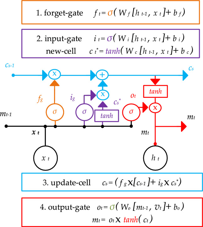
LSTM architecture.
Within the LSTM framework, four distinct layers ensure the systematic data flow. This is in addition to the trio of gates that manage the information within the cell state, denoted as cs. In the preliminary layer, the ‘forget-gate’ fg evaluates the preceding cell state cs-1, to decide the extent of data from cs-1 to be retained in the current state, cs. During this evaluation, fg processes the output from the earlier block m(t − 1) and the feature vector of the present instance (vt), yielding a value between 0 and 1 for every element in the previous cell state—where 0 signifies a definite discard and 1 denotes complete retention.
Proceeding to the next layer, the ‘input-gate’ ig, aided by the sigmoid function, designates the quantity of information from vt to be retained within the cell state. Simultaneously, a hyperbolic tangent layer formulates an additional candidate vector *cs, encapsulating potential values for integration into the cell state. The values from ig and *cs are then combined through a multiplication operation, followed by their incorporation into the current state via summation, leading us to the third layer. Here, the cell state undergoes an update by assimilating new insights and shedding outdated information.
Concluding the process, the fourth layer focuses on the extraction and display of pertinent details as a part of the output. To achieve this, the layer employs a sigmoid function (highlighted in red) for optimal data selection. Subsequently, the cell state undergoes a transformation via the hyperbolic tangent operation (tanh) and gets scaled by the output of the sigmoid function, denoted by σ(x) = (1 + e−x)−1, resulting in Ot. In this context, Ot refines cs into the vector mt making the cell state’s memory accessible to the broader network. Throughout any sequence data timestep (t), Wf, Wi, Wc, and W0 symbolize adjustable weight matrices, while bf, bi, bc, and b0 represent their associated bias terms.
Adaptive moment estimation (Adam) optimizer is employed for parameter updates, including weights and biases34. Adam, conceived as an enhanced iteration of the stochastic-gradient-descent (SGD) optimization technique, has gained traction in recent deep-learning model training endeavors25. Benefiting from the strengths of both root-mean-square-propagation (RMSprop) and adaptive gradient methodologies (AGM), Adam introduces an additional momentum component for optimal parameter adjustment. In a similar way, when updating parameters within LSTM, the SGD optimizer strives to reduce the loss function, which can be articulated as in (16):
| 16 |
In (16), n signifies the number of iterations. The learning rate is represented by α, while the term represents the parameter vector. Additionally, the loss function evaluated over the training set is denoted by . Within the Adam optimization context, the decay averages for previous gradients are represented as Sn and for historical squared gradients as Tn as expressed in (17) and (18):
| 17 |
| 18 |
Here, β1 and β2 represent decay rates. However, it is observed that during initialization, Sn and Tn are biased towards zero, especially when decay rates are low. Therefore, Adam employs moving averages to update the network parameters, and the most precise model is obtained when the loss function is minimal. Hence, the loss function is restructured as follows:
| 19 |
To achieve optimal training outcomes, the parameters are set to default values: β1 = 0.9, β2 = 0.999, and epsilon (ε) is configured to 10–835.
Implementation of the proposed algorithm
This section presents the implementation of the BO-based LSTM algorithm for HVDC fault protection and classification.
Collection of data
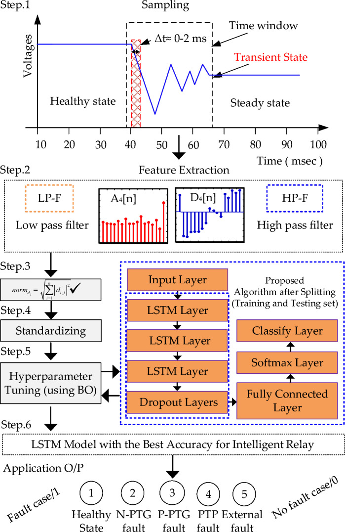
The depicted LSTM-based algorithm is illustrated in Fig. 8, showcasing the architecture utilized for HVDC fault protection. To collect training data that represents all possible fault scenarios, time windows (0–1 ms, 0–1.5 ms, 0–2 ms) are used in PSCAD/EMTDC to collect data samples with varying fault resistance and fault distance. Table 2 shows the modified HVDC system parameters for the training samples. To improve the algorithm’s generalization ability for Fint, kI represents each class of the three DC-line fault types (N-PTG, P-PTG, and PTP), with each class accounting for one-third of Fint. Faults at line 13 are studied for training and testing.
Figure 8.
Proposed algorithm based on an LSTM approach.
Table 2.
HVDC parameters for training datasets.
| Variable | Values |
|---|---|
| Location (km) for internal faults | 1, 10, 20, 30, 40, 50, 60, 70, 80, 90, 110, 120, 130, 140, 150, 160, 170, 180, 190, 198, Total number of fault location values: L = 20 |
| Fault-resistance (Ω) for internal faults | 0.01, 0.1, 0.2, 0.5, 1, 5, 15, 25, 55, 75, 100, 125, 175, 200, 250, 275, 300, 325, 350, 375, 400. Total number of fault resistance values: R = 21 |
|
External-fault types (AC faults) Each character set except G (stands for ground) represent phase AC faults occurred at AC wind farm 1 (Converter 1) |
Three-Phase to Ground (ABCG) with fault resistance range (0.01, 0.1, 1, 5, 10, 15, 25, 50, 75,100, 125, 175), Two-Phase to Ground (ABG, ACG, BCG), Single-Phase to Ground (AG, BG, CG), Phase to Phase (AB, AC, BC) with fault resistances: 0.1, 5,10, 15, 20, 25, 30. Total AC faults = 12 + 21 + 21 + 21 = 75 |
| External-fault types (DC bus faults) | Fault resistances: 0.01, 0.1, 1, 5, 10, 15, 20, 25, 30, 35, 40, 45, 50,…, 375, 380, 385, 390, 395, 400,…, 595,600, 605, 610. Total DC bus faults are 125 |
| Noise-(dB) | 20, 25, 30,45 |
|
Healthy State (100) + External fault types (125 + 75) = 100 + 200 = 300 Total Internal faults (Fint) = (kI × 3) = 420 × 3 = 1260 |
kI = L × R = 20 × 21 = 420/each Fint fault type, 3 Fint faults types (i.e. N-PTG = 420, P-PTG = 420, PTP = 420), Training samples = [(Fint = kI × 3) + 300] = N = 1560, Training samples = 1560 for training only |
There are three windows, each window will be trained for 1560 samples. Total samples 1560 × 3 = 4680 are given to classifier. Time windows (0–1 ms, 0–1.5 ms, 0–2 ms).
Standardization
The Daubechies wavelet with a coefficient of four is employed, chosen for its close alignment with the fault signal pattern denoted by X32. Subsequently, this information is introduced into the input layer for training purposes, where X comprises various subsets [X1, X2,…, Xn]; each Xg represents a fault type or a healthy state qg within [q1, q2,…,qn]. A feature standardization step is performed before splitting the total samples into training and testing sets to reduce differences between the original and transformed data. This process narrows the divergence and enhances the convergence rate, thereby facilitating improved model training. The standardization procedure is given by (20):
| 20 |
Here, N* denotes the processed dataset supplied to the proposed algorithm. Ni stands for the input data and signifies an average of the samples. Simultaneously, S represents the standard deviation of the input data.
Architectural configuration
In the subsequent phase, the devised model comprehends the association between the input (Xg) and output (qg) patterns through offline training, utilizing the training dataset to categorize the DC faults. This process is articulated mathematically as expressed in (21).
| 21 |
In this context, ℝ signifies the LSTM function, and Xg is elaborated as [xg1, xg2,…., xgL]. Each xg j is a column vector denoting feature inputs with a length of L data (equivalent to the length of time) introduced into the input layer. To leverage the temporal features of LSTM, qg needs to be extended to the identical length as Xg, forming the row vector Qg = [qg, qg,…., qg]. Here, L represents the length of the row vector.
Now, the data is arranged as in (22) and (23):
| 22 |
| 23 |
In this scenario, three fault types—PTP, N-PTG, and P-PTG—alongside external faults and healthy operation are designated target types as expressed in (24) and (25).
| 24 |
| 25 |
Following the designation of target types, the preprocessed data transforms a feature vector via the input layer of the proposed algorithm. To capture underlying data features efficiently, we have integrated LSTM layers with the help of BO implementation. The output from the hidden LSTM layer then proceeds to a fully connected layer, where refined information is categorized into different classes. Subsequent application of softmax and classification layers aids in distinguishing between normal and abnormal states in the MT-HVDC system52,53. As fault operating conditions are dynamic, it becomes difficult to incorporate all fault scenarios, resulting in an insufficient number of training samples. Because of this limitation, traditional LSTM models may be prone to overfitting, which is amplified by the inefficient hit-and-trial method for hyperparameter selection. Consequently, the subsequent sub-section offers a comprehensive exploration of these challenges and outlines the criteria employed to mitigate them.
Addressing overfitting challenges
In fault classification, overfitting poses a significant challenge, mainly when dealing with infrequent occurrences in the available samples12. Large neural networks trained on a limited dataset tend to overly adapt to the training data. While one approach to mitigate this is fitting various neural networks on the same dataset and averaging predictions, this is not feasible for the expansive scale of the MT-HVDC system. An alternative effective solution to counter overfitting, especially in the context of the MT-HVDC system, is the application of dropout, as suggested in the literature36.
To counter overfitting effectively, the introduction of dropout stands out as a crucial solution36. As a regularization method, dropout entails training an LSTM layer with multiple sub-networks, averaging their outcomes. These sub-networks, distinct for each iteration, drop out neurons from the original network with a defined probability (P). This strategy prevents the proposed algorithm from excessively fitting the training set, and for these reasons, dropout is incorporated after every LSTM layer to enhance the fault classification process.
Bayesian optimization for LSTM hyperparameter tuning
LSTM networks, a specialized form of RNNs, are equipped with complex architectures that are particularly well-suited for sequence-based tasks. However, determining these models’ optimal set of hyperparameters can be computationally prohibitive. Traditional search methods, such as grid search (GS) and random search (RS), are resource-intensive and often fall short of efficiently optimizing the hyperparameter space. To address this challenge, BO has become an effective optimization method that builds a probabilistic model to locate the optimal hyperparameters accurately. For LSTMs, these hyperparameters include but are not limited to the number of LSTM units, the number of layers, learning rate, dropout rate, and batch size54.
BO is a sophisticated, model-based approach designed to optimize black-box objective functions that are computationally expensive to evaluate. Rather than applying brute-force exhaustive searches, this method leverages prior objective function evaluations to construct a probabilistic model. The model is then utilized to determine the most promising point for the subsequent function evaluation, striking a delicate balance between exploring regions with high uncertainty and exploiting regions with low estimated objective values.
The Gaussian Process (GP), a non-parametric probabilistic model employed to model the distribution over possible objective functions, is central to BO. A GP is fully characterized by its mean function m(x) and its covariance function k(x,x′), commonly called the kernel. Given a dataset consisting of input–output observations, the GP furnishes a posterior distribution over functions when combined with this data. For any new point , the Gaussian Process (GP) predicts a Gaussian distribution with mean μ() and variance σ2(x∗) defined as follows in (26) and (27):
| 26 |
| 27 |
where, is a vector consisting of the covariances between and every point in X. Noise term accounting for observational noise is denoted by . Lastly, I is the identity matrix.
Acquisition function
The Acquisition Function, often denoted as a(x), plays a pivotal role in BO by serving as a decision-making heuristic. Its primary function is to guide the optimization algorithm in selecting the next point x in the hyperparameter space to evaluate. The acquisition function quantifies the expected utility or improvement of evaluating the objective function at a particular point x, based on the existing data and the probabilistic model, such as the Gaussian model considered in this study. The Acquisition Function operates by considering two fundamental criteria: exploration and exploitation. Exploration investigates regions in the hyperparameter space where the uncertainty σ(x) is high, allowing the model to explore new regions that could potentially yield better results. In contrast, exploitation capitalizes on regions where the estimated objective value μ(x) is low (assuming minimization), aiming to refine the search around promising points.
The decision for the next point x to evaluate is usually determined by maximizing a(x):
| 28 |
Several types of acquisition functions have been utilized in literature, such as the probability of Improvement (PI), Expected Improvement (EI), and Upper Confidence Bound (UCB). This study elaborates on a modified EI version and its mathematical formulation. EI aims to find a trade-off between exploration and exploitation based on the current probabilistic model. However, it often does not account for the computational cost. Therefore, an adapted version, known as Expected Improvement per Second (EIps), and its further refinement, Expected Improvement per Second Plus (EIps+), is employed in this study.
The Classical EI at point x can be expressed mathematically as in (29):
| 29 |
In (29), Z is calculated as:
| 30 |
where is the mean prediction of the objective function at x based on the GP model. The standard deviation (uncertainty) at x, also based on the GP model, is represented by . It is the best objective value observed so far. The cumulative distribution function (CDF) of the standard normal distribution is denoted by . Lastly is the standard normal distribution’s probability density function (PDF). The term encapsulates the trade-off between exploration and exploitation. When σ(x) is high (indicating uncertainty), the acquisition function leans towards exploration. Conversely, exploitation is favoured when μ(x) is significantly lower than f(x+).
For EIps+, the evaluation incorporates the expected computational time s(x) as in (31):
| 31 |
where represents the uncertainty in computational time and a hyperparameter mediates the trade-off between expected improvement and the uncertainty in computational time. This extensive approach provides a comprehensive framework for employing BO to fine-tune LSTM hyperparameters, balancing performance and computational efficiency.
Tuning of hyperparameters
In the proposed algorithm, we tune hyperparameters such as the learning rate, the number of LSTM units, the number of layers, batch size, and dropout rates. Table 3 presents the range of hyperparameters and selected values. Search space was also carefully selected to reduce the computational complexity and balance exploration and exploitation. The training phase of the model relies heavily on the BO method. Throughout the training process, the model’s performance is consistently evaluated against a validation set using the Mean Absolute Error (MAE) as the metric of choice.
| 32 |
Table 3.
Range (search space) and selected values of hyperparameters.
| Hyperparameter | Range | Selected value |
|---|---|---|
| Learning rate | 1 × 10⁻⁵ to 1 × 10⁻² | 0.009 |
| Number of LSTM units | 50 to 500 | 129 |
| Number of layers | 1 to 3 | 3 |
| Batch size | 16 to 256 | 32 |
| Dropout rate | 0 to 0.5 | 0.5 |
In Eq. (32), the term MAE refers to the Mean Absolute Error, “TDNP” signifies the total number of data points, and Ya and Y∗a represent the predicted and actual DC fault types, respectively. Subsequently, the model that achieves the lowest MAE on the validation set is further assessed on a distinct test set to ensure its Optimization remains robust and broadly applicable.
The learning rate adjusts the model weights with respect to the loss gradient. It controls the step size taken during the optimization process in training. Within a spectrum of 1 × 10⁻⁵ to 1 × 10⁻², the chosen value of 0.009 is near the higher end. BO has found that this learning rate led to faster convergence without causing instability in the training process. This suggests that the model could benefit from significant weight updates without overshooting the optimal weights. The number of LSTM units refers to the number of neurons or cells in a single LSTM layer of a recurrent neural network. It reflects the ability of the layer to capture and retain information over time. In the range of 50 to 500, 129 is a moderate choice. BO might have determined that this number of units provided a good trade-off between model complexity and the risk of overfitting, capturing the necessary patterns in the data without becoming too large. The number of Layers indicates the depth or number of LSTM layers stacked in sequence in the network. More layers allow the model to recognize more complex features and sequences. From the range of 1 to 3, BO chose the maximum of 3 layers, suggesting that a deeper model was more effective for this particular problem, potentially capturing intricate patterns or hierarchies in the data.
The batch size denotes how many data samples the model processes together in a single pass during training. Out of a range from 16 to 256, a batch size of 32 implies that smaller batches resulted in better or faster convergence for the model in this context. Smaller batches can sometimes lead to noisier gradient updates, which can aid in avoiding local minima. Dropout is a regularization technique where a set fraction of the neurons is rendered inactive (“dropped out”) during training to mitigate overfitting. The dropout rate specifies this fraction. With a range from 0 to 0.5, the chosen rate of 0.5 is high. BO likely determined that the network required strong regularization to prevent overfitting and perform well on unseen data.
Using BO with the EIps + acquisition strategy, we finely tuned our model’s hyperparameters over 30 iterations. This combination, rooted in the EIps + approach, efficiently navigated the hyperparameter space while optimizing computational efficiency. As a result, the model achieved robust performance metrics, including a training MAE of 100%.
Proposed protection scheme
The architectural framework of the proposed protection mechanism, employing BO-based LSTM models, and the proposed single trained unit are illustrated in Fig. 9. A Phase Measurement Unit (PMU) continually acquires analogue signals, incorporating a sampling circuit. These signals then undergo Analog-to-Digital (A/D) conversion and are stored in memory circuits. Subsequently, these digitized signals are relayed to the signal processing unit, where real-time WT is replaced by multi-time window LSTM analysis. The LSTM model, optimized explicitly for hyperparameters using BO, processes these input vectors within predefined time windows of 1 ms, 1.5 ms, and 2 ms to accurately identify internal faults in the designated zone.
Figure 9.
Diagram illustrating the integrated protection scheme featuring Bayesian Optimization-based LSTM models.
An integrated validation unit is incorporated to synchronize the operation of both primary and secondary LSTM units to enhance system reliability. This validation mechanism ensures that the secondary unit acts only when necessary. For instance, in a phase-to-phase (P–P) fault, the primary unit first assesses input vectors within a 1 ms time window to decide whether a trip signal (Tmain) should be issued. A successful trip operation by the primary unit sets a monitored variable ℎ to 1, turning off subsequent action from the secondary unit. However, challenges such as inaccurate relay settings or unknown system parameters can affect the primary unit’s performance. For example, a far-end fault with a high fault resistance value can reduce the peak transient current, making it difficult for the primary unit to detect the fault. If the primary unit fails, the system relies on the secondary LSTM unit or the tertiary LSTM unit if necessary. The secondary and tertiary LSTM units operate on longer time windows of 1.5 ms and 2 ms, respectively. In the event of a primary unit failure, indicated by the variable ℎ being set to 0, the optimized BO-based secondary LSTM unit takes over. It issues a trip command (Tsec) within a 1.5 ms time window to the corresponding Hybrid HVDC circuit breaker (H-DCCB). This multi-time window approach enhances the protection scheme’s robustness and adaptability, particularly in situations where the primary unit’s timely response is hindered. The same collaborative mechanism is proposed between secondary and tertiary units to handle failures if secondary LSTM units fail.
Evaluation of the proposed protection mechanism
The assessment of the scheme’s effectiveness comprises two distinct phases: model training and subsequent testing. The model is rigorously evaluated after offline training using test samples that fall within the parameter boundaries established during training. Table 4 delineates the spectrum of fault characteristics and the types of faults considered for these test samples. Subsequent subsections detail the results, presenting insights into the model’s performance under various faulty and non-faulty conditions.
Table 4.
Parameters of the HVDC grid utilized for evaluation.
| HVDC parameters | Parameter values |
|---|---|
| Location (km) | 15, 25, 55, 125, 155, 165, 175, 185, 195 km, L = 9 |
| Fault-resistance (Ω) | 10, 50, 110, 160, 210, 260, 360, 380, 450, 480 Ω, R = 10 |
|
External-fault types (Fext) Each character set except G (stands for ground) represents phase. Total DC bus faults are 11. Total AC faults are 10. Total Fext = 11 + 10 = 21. AC faults occurred at AC wind farm 1 (Converter 1) |
DC Bus Faults with fault resistances: 8, 22, 34, 42, 54, 62, 74, 82, 94, 102, 114 Ω |
| Three-Phase Faults (ABCG) with fault resistances: 6, 8, 12 Ω | |
| Two-Phase Faults: ABG: 6 Ω, BCG: 8 Ω, CAG: 6 Ω, AB: 8 Ω | |
| Single-Phase to Ground Faults: AG: 6, BG: 8 Ω, CG: 12 Ω | |
| Noise-(dB) | 20, 25, 30, 45 |
| Healthy State + External fault = 21 + 21 = 42 | kI = R × L = 90/each Fint fault type, 3 Fint faults types (i.e. N-PTG = 90, P-PTG = 90, PTP = 90), Total Internal faults (Fint) = (kI × 3) = 90 × 3 = 270, Testing samples = [Fint + 42] = kE = 312 for each window, Testing samples = 312 for testing each window only |
Assessment of performance under different fault locations and impedances
In this segment, we evaluate the efficacy of our proposed method in handling DC-line faults. We chose a sample size of kE = 312 to ensure a balanced representation of each fault category. The criteria detailed in "Implementation of the proposed algorithm" guided this choice, ensuring a holistic appraisal of accuracy. For internal faults like PTP and PTG, the dB-4 wavelet-derived sub-band was consistently identified for every test set of Fint (kI × 3 = 270), irrespective of changes in fault resistance or distance. This yielded a notable accuracy rate of 99.04%, which can be referenced in Table 5. In situations like Fext or during the standard grid operation, the system effectively identified the protected line as fault-free across all the fault scenarios examined.
Table 5.
Fault identification accuracy for 2 ms window.
| Fault types | Total faults | Identified faults | Misclassified faults | Accuracy (MAE) | Internal fault | External fault |
|---|---|---|---|---|---|---|
| PTP | 90 | 89 | 1 | 98.9% | ✓ | X |
| P-PTG | 90 | 89 | 1 | 98.9% | ✓ | X |
| N-PTG | 90 | 89 | 1 | 98.9% | ✓ | X |
| External faults | 21 | 21 | 0 | 100.0% | X | ✓ |
| Healthy | 21 | 21 | 0 | 100.0% | X | X |
The inception angles ranged from 0° to 360° in steps of 15°, ensuring that faults were initiated at different points in the AC cycle. Then, 10 random external AC faults were picked accordingly with 0.3 s fault duration. Note that our focus is on feature extraction from DC signals for DC transmission line faults. We recognize the importance of feature extraction for three-phase signals and will consider this in future work. There are three windows, so the total number of testing samples is 936 (Total = 312 × 3 = 936). Faults at line 13 are studied for training and testing.
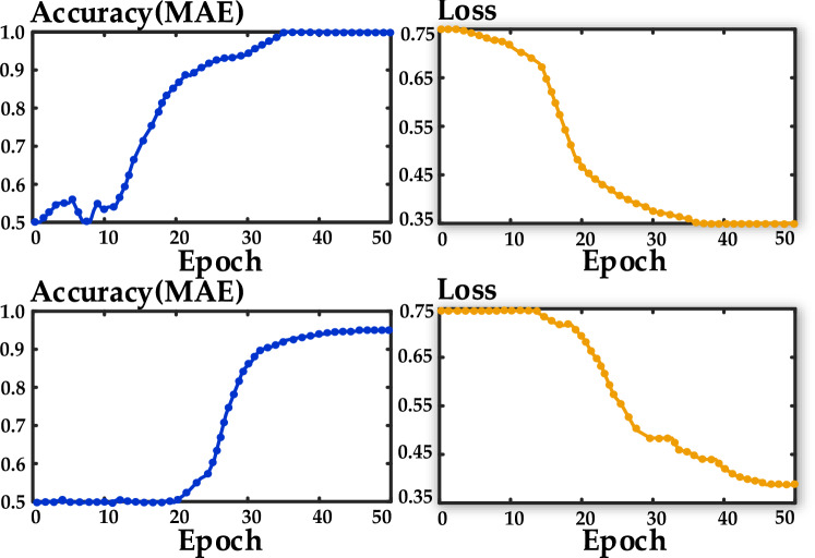
The visual representation in Fig. 10 demonstrates that the proposed model’s fault classification accuracy improves at a commendable rate during its training phase as the loss function diminishes. The algorithm’s ability to recognize long-term patterns, delve deeply into unique fluctuations, and maintain an optimal starting learning rate contributes to this improvement. Consequently, it outperforms the traditional LSTM algorithm in terms of convergence speed and precision. The model was tested on a machine equipped with MATLAB R2019a, and it took 133 s for training.
Figure 10.
Comparison of accuracy and loss function between the proposed model and traditional LSTM.
Efficiency under noisy conditions
Even with the advent of enhanced signal processing components like filtering algorithms and optical instrument transformers in contemporary relay systems, noise remains a factor that could affect the performance of protection algorithms. We incorporated white Gaussian noise with a Signal Noise Ratio ranging from 20 to 45 decibels into all test measurements to evaluate how well our algorithm withstands and performs in varying noisy conditions. This produced ‘kn’ test samples, each comprising four distinct kinds of noise-affected data, each containing ‘kE’ samples. Figure 11 depicts the impact of a 20 dB noise level.
Figure 11.
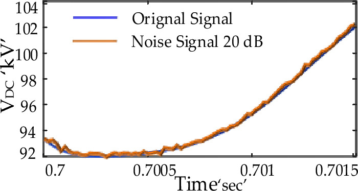
Effect of 20 dB noise on the original signal.
Figure 12 provides an evaluation using solely 20 dB noise samples, with each row signifying the predicted categories and each column indicating the actual categories. The bottom rows of Fig. 12 display how well our algorithm performs for each specific fault type, as evidenced by the confusion matrix. The total accuracy of the system stands at 95.5%, as indicated in the bottom-right cell of the matrix.
Figure 12.
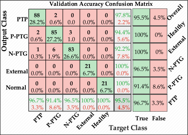
Confusion matrix of the proposed algorithm in case of 20 dB noise for 2 ms window.
In sequence, Table 6 outlines the classification accuracy for individual fault types across a noise spectrum ranging from 20 to 45 dB. The data reveals that the total classification accuracy experiences a mere 4% reduction, which is acceptable. The optimization of the algorithm’s hyperparameters, including the learning rate, during the offline training phase, accounts for noise factors, thereby contributing to its resilience. Consequently, the intelligent model maintains its efficacy without encountering any operational issues.
Table 6.
Fault detection accuracy in noisy environments for 2 ms window.
| Fault types | Accuracy (20 dB) | Accuracy (25 dB) | Accuracy (30 dB) | Accuracy (45 dB) |
|---|---|---|---|---|
| PTP | 96.7% | 96.7% | 97.7% | 98.9% |
| P-PTG | 91.4% | 92.5% | 93.5% | 95.7% |
| N-PTG | 96.5% | 97.7% | 97.7% | 98.9% |
| External faults | 100.0% | 100.0% | 100.0% | 100.0% |
| Overall accuracy | 95.5% | 96.2% | 96.8% | 98.1% |
Comparative analysis against conventional approaches
In order to gauge the effectiveness and accuracy of our proposed algorithm, we substituted it with conventional LSTM and BP-NN methods. The testing conditions remained consistent with those described in Table 4. Figure 13 visualizes the findings. For a comprehensive accuracy assessment, we employed the fault resistance values in Table 5 at various fault distances—specifically at 15, 25, 55, 125, 155, 165, 175, 185, and 195 km.
Figure 13.
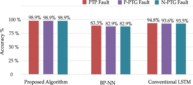
Comparison with existing methods for 2 ms window.
The data in Fig. 13 reveals that our proposed algorithm outperforms BP-NN in accuracy. Upon completion of the training phase, our model required 950 iterations at a learning rate of 0.009, achieving a training accuracy of 100%. In contrast, the traditional LSTM model necessitated 2120 iterations and reached a training accuracy of 98.40%, using a learning rate of 0.03 determined through trial and error. These metrics indicate that our algorithm trains more rapidly.
Table 7 shows the fault detection accuracy under different time windows. In comparison, our model achieves optimal results across epochs thanks to optimized parameters like mini-batch size, which accelerate training without compromising accuracy. Additionally, our model avoids underfitting and overfitting, common problems in poorly-tuned neural networks.
Table 7.
Fault detection accuracy under the different time windows.
| Different time windows | BO-LSTM Model | Simple LSTM | BP-NN |
|---|---|---|---|
 1ms Window 1ms Window |
98.4% | 96.2% | 82.1% |
 1.5ms Window 1.5ms Window |
98.9% | 96.7% | 82.8% |
 2ms Window 2ms Window |
99.04% | 97.8% | 83.0% |
| Overall | 98.8% | 96.9% | 96.0% |
LSTM-based protection coordination with DC circuit breakers: evaluation and validation
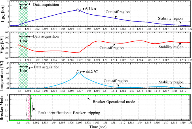
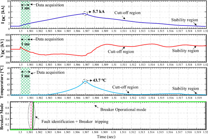
To validate the coordination between the primary unit and the H-DCCB, we introduce a fault scenario at t = 1.5 s on Line 13 (L13), which is 125 km from MMC 3. This fault scenario features a low impedance point-to-point (PTP) fault with a resistance of 10 Ω. An initial triggering element (Tset) is activated upon a sudden current increase, as shown in Fig. 14, initiating the data collection phase. Utilizing LSTM algorithms, the primary unit generates a circuit breaker trip command (Tmain) by analyzing input vectors within a 1 ms time frame. The time required for this operation was approximately 500 μs in our computational setup. An additional computational delay of 1 ms may be incorporated to simulate commercial protection devices. Prior to the fault, the current flow through the breaker was measured to be around 0.5 kA. Within a 1 ms window, the primary unit calibrates itself to identify abrupt elevations in fault current—up to three times the rated current—and subsequently issues a trip command to the H-DCCB. The resultant fault current peaks at approximately 6.2 kA, substantially lower than the 16 kA interrupting capacity suggested in33. Notably, the proposed LSTM-based protection strategy maintains the IGBT (Insulated Gate Bipolar Transistor) valve of the main breaker within permissible temperature limits, affirming its ability to isolate low-resistance faults expeditiously and reliably when implemented in conjunction with DCCBs.
Figure 14.
Integration of the proposed protection with DCCBs (primary unit).
For a more rigorous validation of the LSTM-based protective strategy, we extend our tests to ascertain the isolation of only the faulted line. We conducted a comprehensive study after training relevant parameters via our LSTM algorithm. We triggered an internal PTP fault with 40 Ω fault impedance at t = 1.5 s on Line 14 (L14), which is 110 km away from MMC 4. The instant the fault manifests, a sharp decrease in system voltage is recorded. When the rate of voltage change exceeds a predetermined level, the initial triggering element (Tset) is activated, launching the data acquisition process.
The primary unit generates a trip command (Tmain) to the breaker using input vectors assessed within 1 ms. As evidenced in Fig. 15, the primary protective mechanism effectively activates on L14, leading to a peak fault current of 5.7 kA—still well below the 16 kA stated in33. Consequently, the DCCBs function to isolate the fault on L14 effectively.
Figure 15.
Integration of the proposed protection with DCCBs (generalized case study).
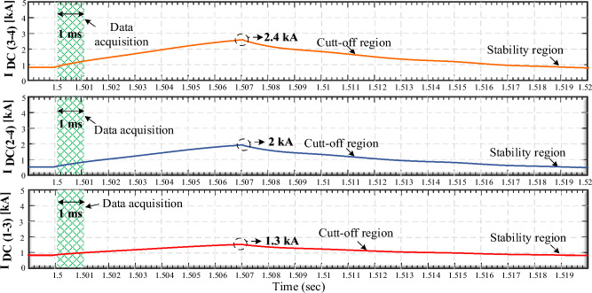
One must ensure that the initial triggering element (Tset) does not activate for H-DCCBs on adjacent lines to maintain the specificity of the protective mechanism. This has been corroborated by monitoring the currents on lines L24, L34, and L13 while the fault occurs on L14, as illustrated in Fig. 16. Consequently, the LSTM protection strategy remains dormant, preventing unnecessary tripping of H-DCCBs on the aforementioned healthy lines (Fig. 17).
Figure 16.
Integration of the proposed protection with DCCBs (Monitoring lines L24, L34, and L13 during fault initiation on L14).
Figure 17.
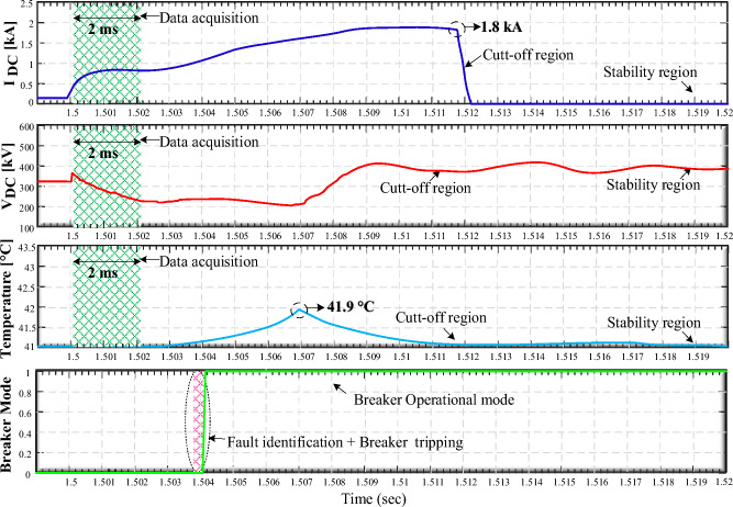
Integration of the proposed protection with DCCBs (tertiary unit protection).
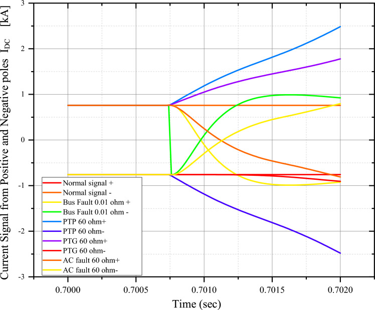
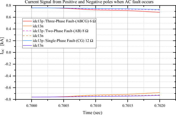
For segregation, show normal and fault conditions under dissimilar fault cases. Please refer to the Fig. 18, Fig. 19 and Appendix (supplementary material section). Figure 20 shows effects of AC faults on DC signals.
Figure 18.
Normal conditions and fault conditions under some dissimilar fault cases.
Figure 19.
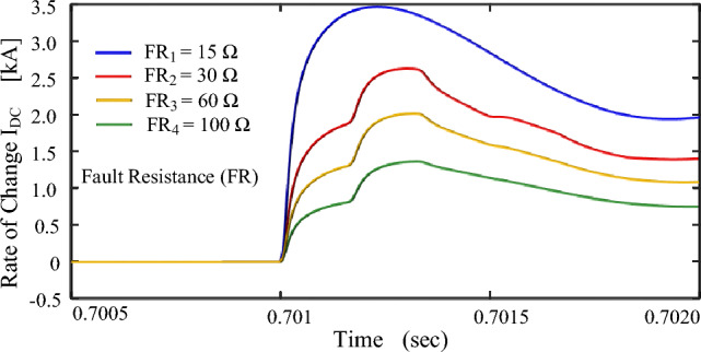
Shows the rate of rise for IDC in an internal fault during different fault impedances.
Figure 20.
Shows the effect on IDC during different external AC faults.
For the subsequent phase of the validation process, we examine the secondary unit by introducing a high-resistance fault (P-PTG) with a 110 Ω impedance at 55 km away from MMC 3 on L13. High-impedance faults typically yield attenuated transient fault currents, requiring the secondary unit to monitor abnormal rises in current for extended durations without overstressing the thermal limits of the IGBT valves. These valves represent some of the most delicate and costly components of H-DCCBs. Figure 17 displays the secondary unit’s capability to monitor abnormal current surges for 2 ms following fault inception. A breaker trip sequence is executed upon fault identification, resulting in a maximum fault current of 1.8 kA. The IGBT valves maintain voltage fluctuations within 1.5 times the rated system voltage, inflicting minimal thermal and electrical stress and ensuring no damage is incurred.
Comparative assessment of traditional and non-traditional approaches
AI-based approaches
Table 8 underscores the fault-detection algorithm’s resilience in various dimensions, such as noise immunity, system complexity, and fault tolerance, compared to existing AI-based techniques16,37–39. A crucial aspect of our discussion centers on finding the optimal trade-off among detection accuracy, time-window length, and response speed. Shorter time windows (e.g., 1–3 ms) are generally favored in AI-based methods for high-speed responses in high-voltage DC protection37–39. Nevertheless, the volatile and intricate operational environment of the MT-HVDC system tends to make these conventional, simpler AI models susceptible to convergence issues, adversely affecting their detection accuracy.
Table 8.
Comparison with AI methods.
| Protection method | Detection-method | Feature selection | Noise immunity (dB) | Fault resistance withstanding ability | Sampling-rate | Pre-training settings | Complexity in training setup time | Other remarks | Average-recognition rate |
|---|---|---|---|---|---|---|---|---|---|
| Ref.37 | ANN | DWT | High (18.0 dB) | High (350.0 Ω) | Medium | Trial and error | Medium | A generalized linear model to set up hyperparameters of a non-linear model causes miss-convergence at a small window length | 90.61% |
| Ref.16 | ANN | Voltages | Low | Low (50.0 Ω) | Low | Trial and error | High | Due to the large window length, response time is slow | 94.35% |
| Ref.38 | SVM | WT | Not mentioned | Low | High | Not mentioned | High | Do not discuss noise immunity in the complicated and dynamic environment of the MT-HVDC networks | 92.92% |
| Ref.39 | ANN | Fast FT | Low (50.0 dB) | Low (100.0 Ω) | Medium | Trial and error | Medium | An in-depth analysis of noise immunity is missing, and the fault resistance range is -0.01–100-Ω- | 88.85% |
| Proposed methodology | Improved LSTM | Norm | High (20.0 dB) | High (480.0 Ω) | Medium | Optimal settings (BO) | Low | Due to the optimal training solution, it is less prone to miss-convergence at a small window length | 99.04% |
Some studies16,40,41 have attempted to mitigate this by extending the time window to a range between 10 and 40 ms, but this adjustment typically results in slower response times. Achieving a harmonious balance among detection accuracy, time-window length, and response speed becomes essential for optimal performance. Considering this, we compared various intelligent methods under identical test conditions, as outlined in "Efficiency under noisy conditions". Our proposed algorithm stands out due to its advanced feature selection process, inclusion of dropout layers, and efficient hyperparameter optimization strategy. The algorithm fully leverages the inherent strengths of LSTM, such as example-based learning, pattern classification, and a high ability to generalize. These attributes are hard to replicate when using other models with abbreviated time windows, as shown in Table 8.
In MT-HVDC systems, the self-tuning feature of our suggested algorithm provides both time and cost efficiency. This is particularly beneficial given that manually configuring parameters for a complex, intelligent relay system often necessitates specialized human expertise before training multiple neural network models42. Additionally, Table 8 includes a detailed analytical comparison in its “Other Remarks” section.
Traditional non-AI techniques
Table 9 compares the performance of established traditional non-AI techniques43–51 and our proposed method, emphasizing parametric efficiency. Our model excels in managing high fault resistance without the challenges of sensitivity or operational issues. It further benefits from a reduced sample rate and computational requirement. Additionally, data synchronization isn’t necessary. However, coordination between protection and control is a limitation that needs investigation48.
Table 9.
Comparison with non-AI methods.
| Protection method | Detection method | Fault resistance | Noise issue | Sampling rate (kHz) | Communication link | Calculation rate | Other remarks |
|---|---|---|---|---|---|---|---|
| Ref.43 | Overcurrent criteria | Low (5.0 Ω) | Yes | 100.0 | No | Medium | Limited performance in long-distance HVDC transmission |
| Ref.44 | Capacitor-discharging | Low (10.0 Ω) | Yes | 2.0 | Yes | Higher | In a detailed study, we set the fault resistance to zero |
| Ref.45 | DWT | Medium (400.0 Ω) | Yes | 500.0 | No | Medium | The sampling rate is very high |
| Ref.46 - | Voltage change-rate | High | No | 200.0 | No | Lower | Further scrutiny is required to examine bias and the challenges of managing high sampling rates |
| Ref.47 | Threshold barriers via voltage/current signals | Not discussed | Yes | 50.0 | Yes | Higher | Detailed modelling and precise measurements are required to determine a threshold boundary. These models are susceptible to noise signals generated by the measuring instrument |
| Ref.48 | The voltage across bus terminals serves as the basis for establishing threshold barriers | Low (10.0 Ω) | No | 200.0 | Yes | Higher | The classifier must be trained again and reset if some modifications occur in the system suitable for the multivendor application |
| Ref.49 | Naïve Bayes classifier | Low (10.0 Ω) | NA | 10.0 | Yes | Higher | While the operating speed is satisfactory, further investigation regarding high fault resistance is needed |
| Ref.50 | Current differential | Medium (300.0 Ω) | NA | 10.0 | Yes | Small | High fault resistance is studied successfully; unwanted delays to avoid sensitivity and maloperation need consideration |
| Ref.51 | Current signal | Medium (200.0 Ω) | No | 50.0 | No | Medium | A large time window slows down the reaction time |
| Proposed method | Improved LSTM | High (480.0 Ω) | No | No | Low | Read non-AI based methods section |
Conclusions and future research directions
This study introduces a sophisticated LSTM-based protection scheme designed for MMC-HVDC transmission systems. It utilizes multiple time windows of 1 ms, 1.5 ms, and 2 ms for fault diagnosis and classification. BO optimizes the LSTM structure efficiently and effectively. The algorithm generates accurate test results of 99.04%, even under challenging circumstances with noise interference. A simplified and efficient detection process is achieved through our method, unlike traditional approaches that rely on multiple thresholds. The proposed algorithm’s settings are error-free, enabling it to cover failures without relying on back protection. It is efficient to coordinate relays with circuit breakers and issue a trip command (Tsec) within 1.5 ms without adding extra burden. In addition, extensive simulations show that the method is robust to various fault impedances and locations. Since power transmission systems are critical and AI integration is imminent, our findings confirm both the effectiveness of the proposed scheme and its potential for real-world application. Effective synchronization of control and protection mechanisms will be studied in the future. This can help to improve HVDC grid protection with a faster and more robust response.
In the next stage of our research, we plan to rigorously test our Bayesian-Optimized LSTM-DWT fault detection model using Real Time Digital Simulator (RTDS) technology. This step is critical to confirm that our model performs reliably under real-world conditions that mirror the complexities of HVDC systems. We will use RTDS to accurately measure how quickly and effectively our model responds to faults, ensuring it meets the high standards necessary for practical use. Additionally, we'll assess the model's robustness by testing its performance against a variety of fault types and disturbances, to guarantee its reliability in actual grid operations. We also aim to explore how well our model can be scaled up for larger, multi-terminal HVDC systems. The insights gained from these RTDS tests will help us refine and improve our model, making it more effective and adaptable. This work will help bridge the gap between theoretical research and practical application, making a significant contribution to advancing fault detection technology in HVDC systems.
Supplementary Information
Author contributions
M.Z.Y., A.R.S.: Conceptualization, methodology, software, visualization, investigation, writing-original draft preparation. S.K., B.H.: Data curation, validation, supervision, resources, writing—review and editing. M.B., I.Z.: Project administration, supervision, resources, writing—review and editing.
Data availability
The datasets used and/or analyzed during the current study are available from the corresponding author upon reasonable request.
Competing interests
The authors declare no competing interests.
Footnotes
Publisher's note
Springer Nature remains neutral with regard to jurisdictional claims in published maps and institutional affiliations.
Contributor Information
Arvind R. Singh, Email: arvindsinghwce@gmail.com
Mohit Bajaj, Email: thebestbajaj@gmail.com.
Ievgen Zaitsev, Email: zaitsev@i.ua.
Supplementary Information
The online version contains supplementary material available at 10.1038/s41598-024-68985-5.
References
- 1.Zain Yousaf, M., Liu, H., Raza, A. & Baber Baig, M. Primary and backup fault detection techniques for multi-terminal HVdc systems: a review. IET Gener. Transm. Distrib.14(22), 5261–5276 (2020). 10.1049/iet-gtd.2020.0060 [DOI] [Google Scholar]
- 2.Khalid, S., Raza, A., Yousaf, M. Z., Mirsaeidi, S. & Zhichu, C. Recent advances and future perspectives of HVDC development in Pakistan: A comprehensive review. IEEE Access11, 56408–56427 (2023). 10.1109/ACCESS.2023.3283431 [DOI] [Google Scholar]
- 3.He, J. et al. A novel directional pilot protection independent of line parameters and boundary elements for MMC-HVDC grid. Int. J. Electr. Power Energy Syst.150, 109094 (2023). 10.1016/j.ijepes.2023.109094 [DOI] [Google Scholar]
- 4.Xiang, W. et al. A transient voltage-based DC fault line protection scheme for MMC-based DC grid embedding DC breakers. IEEE Trans. Power Deliv.34(1), 334–345 (2018). 10.1109/TPWRD.2018.2874817 [DOI] [Google Scholar]
- 5.Luscan, B. et al. A vision of HVDC key role toward fault-tolerant and stable AC/DC grids. IEEE J. Emerg. Sel. Top. Power Electron.9(6), 7471–7485 (2020). 10.1109/JESTPE.2020.3037016 [DOI] [Google Scholar]
- 6.Shao, B. et al. Power coupling analysis and improved decoupling control for the VSC connected to a weak AC grid. Int. J. Electr. Power Energy Syst.145, 108645. 10.1016/j.ijepes.2022.108645 (2023). 10.1016/j.ijepes.2022.108645 [DOI] [Google Scholar]
- 7.Li, B., He, J., Li, Y. & Li, B. A review of the protection for the multi-terminal VSC-HVDC grid. Prot. Control Mod. Power Syst.4, 1–11 (2019). 10.1186/s41601-019-0115-7 [DOI] [Google Scholar]
- 8.Zhang, X. et al. Voltage and frequency stabilization control strategy of virtual synchronous generator based on small signal model. Energy Rep.9, 583–590. 10.1016/j.egyr.2023.03.071 (2023). 10.1016/j.egyr.2023.03.071 [DOI] [Google Scholar]
- 9.Huai, Q. et al. Backup-protection scheme for multi-terminal HVDC system based on wavelet-packet-energy entropy. IEEE Access7, 49790–49803 (2019). 10.1109/ACCESS.2019.2910384 [DOI] [Google Scholar]
- 10.Ouyang, J. et al. A predictive method of LCC-HVDC continuous commutation failure based on threshold commutation voltage under grid fault. IEEE Trans. Power Syst.36(1), 118–126 (2020). 10.1109/TPWRS.2020.3001939 [DOI] [Google Scholar]
- 11.Jing, X., Wu, Z., Zhang, L., Li, Z. & Mu, D. Electrical fault diagnosis from text data: A supervised sentence embedding combined with imbalanced classification. IEEE Trans. Ind. Electron.71(3), 3064–3073. 10.1109/TIE.2023.3269463 (2024). 10.1109/TIE.2023.3269463 [DOI] [Google Scholar]
- 12.Luo, G., Hei, J., Yao, C., He, J. & Li, M. An end-to-end transient recognition method for VSC-HVDC based on deep belief network. J. Mod. Power Syst. Clean Energy8(6), 1070–1079 (2020). 10.35833/MPCE.2020.000190 [DOI] [Google Scholar]
- 13.Li, S., Zhao, X., Liang, W., Hossain, M. T. & Zhang, Z. A fast and accurate calculation method of line breaking power flow based on taylor expansion. Front. Energy Res.10.3389/fenrg.2022.943946 (2022). 10.3389/fenrg.2022.943946 [DOI] [Google Scholar]
- 14.Meng, X., Chen, W., Mei, H. & Wang, L. Corrosion mechanism of UHV transmission line tower foot in Southern China. IEEE Trans. Power Deliv.39(1), 210–219. 10.1109/TPWRD.2023.3329140 (2024). 10.1109/TPWRD.2023.3329140 [DOI] [Google Scholar]
- 15.Guo, L., Lei, Y., Xing, S., Yan, T. & Li, N. Deep convolutional transfer learning network: A new method for intelligent fault diagnosis of machines with unlabeled data. IEEE Trans. Ind. Electron.66(9), 7316–7325 (2018). 10.1109/TIE.2018.2877090 [DOI] [Google Scholar]
- 16.Merlin, V. L., dos Santos, R. C., Le Blond, S. & Coury, D. V. Efficient and robust ANN-based method for an improved protection of VSC-HVDC systems. IET Renew. Power Gener.12(13), 1555–1562 (2018). 10.1049/iet-rpg.2018.5097 [DOI] [Google Scholar]
- 17.Liu, K. et al. Research on fault diagnosis method of vehicle cable terminal based on time series segmentation for graph neural network model. Measurement10.1016/j.measurement.2024.114999 (2024). 10.1016/j.measurement.2024.114999 [DOI] [Google Scholar]
- 18.Hossam-Eldin, A., Lotfy, A., Elgamal, M. & Ebeed, M. Artificial intelligence-based short-circuit fault identifier for MT-HVDC systems. IET Gener. Transm. Distrib.12(10), 2436–2443 (2018). 10.1049/iet-gtd.2017.1345 [DOI] [Google Scholar]
- 19.Zhao, D., Wang, H. & Cui, L. Frequency-chirprate synchrosqueezing-based scaling chirplet transform for wind turbine nonstationary fault feature time–frequency representation. Mech. Syst. Signal Process.209, 111112. 10.1016/j.ymssp.2024.111112 (2024). 10.1016/j.ymssp.2024.111112 [DOI] [Google Scholar]
- 20.Yang, Q., Li, J., Santos, R., Huang, K. & Igic, P. Intelligent fault detection and location scheme for modular multi-level converter multi-terminal high-voltage direct current. High Volt.6, 125–137 (2020). 10.1049/hve2.12033 [DOI] [Google Scholar]
- 21.Han, Y., Qi, W., Ding, N. & Geng, Z. Short-time wavelet entropy integrating improved LSTM for fault diagnosis of modular multilevel converter. IEEE Trans. Cybern.52, 7504–7512 (2021). 10.1109/TCYB.2020.3041850 [DOI] [PubMed] [Google Scholar]
- 22.Zhang, H., Liu, Z., Huang, G.-B. & Wang, Z. Novel weighting-delay-based stability criteria for recurrent neural networks with time-varying delay. IEEE Trans. Neural Netw. Learn. Syst.21(1), 91–106 (2009). 10.1109/TNN.2009.2034742 [DOI] [PubMed] [Google Scholar]
- 23.Peddinti, V., Wang, Y., Povey, D. & Khudanpur, S. Low latency acoustic modeling using temporal convolution and LSTMs. IEEE Signal Process. Lett.25(3), 373–377 (2017). 10.1109/LSP.2017.2723507 [DOI] [Google Scholar]
- 24.Cai, M. & Liu, J. Maxout neurons for deep convolutional and LSTM neural networks in speech recognition. Speech Commun.77, 53–64 (2016). 10.1016/j.specom.2015.12.003 [DOI] [Google Scholar]
- 25.Wu, Y., Yuan, M., Dong, S., Lin, L. & Liu, Y. Remaining useful life estimation of engineered systems using vanilla LSTM neural networks. Neurocomputing275, 167–179 (2018). 10.1016/j.neucom.2017.05.063 [DOI] [Google Scholar]
- 26.Jayamaha, D., Lidula, N. & Rajapakse, A. D. Wavelet-multi resolution analysis based ANN architecture for fault detection and localization in DC microgrids. IEEE Access7, 145371–145384 (2019). 10.1109/ACCESS.2019.2945397 [DOI] [Google Scholar]
- 27.Qu, N., Li, Z., Zuo, J. & Chen, J. Fault detection on insulated overhead conductors based on DWT-LSTM and partial discharge. IEEE Access8, 87060–87070 (2020). 10.1109/ACCESS.2020.2992790 [DOI] [Google Scholar]
- 28.Cano, A., Arévalo, P., Benavides, D. & Jurado, F. Integrating discrete wavelet transform with neural networks and machine learning for fault detection in microgrids. Int. J. Electr. Power Energy Syst.155, 109616 (2024). 10.1016/j.ijepes.2023.109616 [DOI] [Google Scholar]
- 29.Zhi, S., Shen, H. & Wang, T. Gearbox localized fault detection based on meshing frequency modulation analysis. Appl. Acoust.219, 109943. 10.1016/j.apacoust.2024.109943 (2024). 10.1016/j.apacoust.2024.109943 [DOI] [Google Scholar]
- 30.Liu, L., Zhang, S., Zhang, L., Pan, G. & Yu, J. Multi-UUV maneuvering counter-game for dynamic target scenario based on fractional-order recurrent neural network. IEEE Trans. Cybern.53(6), 4015–4028. 10.1109/TCYB.2022.3225106 (2023). 10.1109/TCYB.2022.3225106 [DOI] [PubMed] [Google Scholar]
- 31.Khalid, S. et al. Technical assessment of hybrid HVDC circuit breaker components under M-HVDC faults. Energies14(23), 8148 (2021). 10.3390/en14238148 [DOI] [Google Scholar]
- 32.Ukil, A., Yeap, Y. M., Satpathi, K. FaultAnalysisandProtectionSystemDesignforDCGrids, 1st ed. (Springer Singapore Pte. Limited, 2020).
- 33.Yousaf, M. Z., Khalid, S., Tahir, M. F., Tzes, A. & Raza, A. A novel dc fault protection scheme based on intelligent network for meshed dc grids. Int. J. Electr. Power Energy Syst.154, 109423 (2023). 10.1016/j.ijepes.2023.109423 [DOI] [Google Scholar]
- 34.Zhao, D., Cui, L. & Liu, D. Bearing weak fault feature extraction under time-varying speed conditions based on frequency matching demodulation transform. IEEE/ASME Trans. Mechatron.28(3), 1627–1637. 10.1109/TMECH.2022.3215545 (2023). 10.1109/TMECH.2022.3215545 [DOI] [Google Scholar]
- 35.Heusel, M., Ramsauer, H., Unterthiner, T., Nessler, B. & Hochreiter, S. Gans trained by a two time-scale update rule converge to a local nash equilibrium. Adv. Neural. Inf. Process. Syst.30, 6626–6637 (2017). [Google Scholar]
- 36.Srivastava, N., Hinton, G., Krizhevsky, A., Sutskever, I. & Salakhutdinov, R. Dropout: A simple way to prevent neural networks from overfitting. J. Mach. Learn. Res.15(1), 1929–1958 (2014). [Google Scholar]
- 37.Xiang, W., Yang, S. & Wen, J. ANN-based robust DC fault protection algorithm for MMC high-voltage direct current grids. IET Renew. Power Gener.14(2), 199–210 (2019). 10.1049/iet-rpg.2019.0733 [DOI] [Google Scholar]
- 38.Luo, G., Yao, C., Tan, Y. & Liu, Y. Transient signal identification of HVDC transmission lines based on wavelet entropy and SVM. J. Eng.2019(16), 2414–2419 (2019). [Google Scholar]
- 39.Yang, Q., Le Blond, S., Aggarwal, R., Wang, Y. & Li, J. New ANN method for multi-terminal HVDC protection relaying. Electric Power Syst. Res.148, 192–201 (2017). 10.1016/j.epsr.2017.03.024 [DOI] [Google Scholar]
- 40.Silva, A. S., Santos, R. C., Torres, J. A. & Coury, D. V. An accurate method for fault location in HVDC systems based on pattern recognition of DC voltage signals. Electr. Power Syst. Res.170, 64–71 (2019). 10.1016/j.epsr.2019.01.013 [DOI] [Google Scholar]
- 41.Abu-Jasser, A., Ashour, M. A backpropagation feedforward NN for fault detection and classifying of overhead bipolar HVDC TL using DC measurements. J.Eng.Res.Technol. 2(3), (2015).
- 42.Baker, B., Gupta, O., Naik, N., Raskar, R. Designing neural network architectures using reinforcement learning. arXivpreprint (2016).
- 43.Yang, J., Fletcher, J. E. & O’Reilly, J. Multiterminal DC wind farm collection grid internal fault analysis and protection design. IEEE Trans. Power Deliv.25(4), 2308–2318 (2010). 10.1109/TPWRD.2010.2044813 [DOI] [Google Scholar]
- 44.Yang, J., Fletcher, J. E. & O’Reilly, J. Short-circuit and ground fault analyses and location in VSC-based DC network cables. IEEE Trans. Ind. Electron.59(10), 3827–3837 (2011). 10.1109/TIE.2011.2162712 [DOI] [Google Scholar]
- 45.Pei, X. et al. A novel ultra-high-speed traveling-wave protection principle for VSC-based DC grids. IEEE Access7, 119765–119773 (2019). 10.1109/ACCESS.2019.2936276 [DOI] [Google Scholar]
- 46.Li, R., Xu, L. & Yao, L. DC fault detection and location in meshed multiterminal HVDC systems based on DC reactor voltage change rate. IEEE Trans. Power Deliv.32(3), 1516–1526 (2016). 10.1109/TPWRD.2016.2590501 [DOI] [Google Scholar]
- 47.Leterme, W., Azad, S. P. & Van Hertem, D. A local backup protection algorithm for HVDC grids. IEEE Trans. Power Deliv.31(4), 1767–1775 (2016). 10.1109/TPWRD.2016.2543306 [DOI] [Google Scholar]
- 48.Sun, J., Saeedifard, M. & Meliopoulos, A. S. Backup protection of multi-terminal HVDC grids based on quickest change detection. IEEE Trans. Power Deliv.34(1), 177–187 (2019). 10.1109/TPWRD.2018.2867787 [DOI] [Google Scholar]
- 49.Raza, A. et al. A protection scheme for multi-terminal VSC-HVDC transmission systems. IEEE Access6, 3159–3166 (2017). 10.1109/ACCESS.2017.2787485 [DOI] [Google Scholar]
- 50.Wang, L., Chen, Q., Xi, C. Study on the traveling wave differential protection and the improvement scheme for VSC-HVDC transmission lines. In 2016IEEEPESAsia-PacificPowerandEnergyEngineeringConference(APPEEC), 1943–1947 (IEEE, 2016).
- 51.Chu, X., Song, G. & Liang, J. Analytical method of fault characteristic and non-unit protection for HVDC transmission lines. CSEE J. Power Energy Syst.2(4), 37–43 (2016). 10.17775/CSEEJPES.2016.00047 [DOI] [Google Scholar]
- 52.Miaofen, L., Youmin, L., Tianyang, W., Fulei, C. & Zhike, P. Adaptive synchronous demodulation transform with application to analyzing multicomponent signals for machinery fault diagnostics. Mech. Syst. Signal Process.191, 110208. 10.1016/j.ymssp.2023.110208 (2023). 10.1016/j.ymssp.2023.110208 [DOI] [Google Scholar]
- 53.Ju, Y., Liu, W., Zhang, Z. & Zhang, R. Distributed three-phase power flow for AC/DC hybrid networked microgrids considering converter limiting constraints. IEEE Trans. Smart Grid13(3), 1691–1708. 10.1109/TSG.2022.3140212 (2022). 10.1109/TSG.2022.3140212 [DOI] [Google Scholar]
- 54.Zhu, D. et al. Rethinking fault ride-through control of DFIG-based wind turbines from new perspective of rotor-port impedance characteristics. IEEE Trans. Sustain. Energy10.1109/TSTE.2024.3395985 (2024). 10.1109/TSTE.2024.3395985 [DOI] [Google Scholar]
Associated Data
This section collects any data citations, data availability statements, or supplementary materials included in this article.
Supplementary Materials
Data Availability Statement
The datasets used and/or analyzed during the current study are available from the corresponding author upon reasonable request.


