

Abstract
Protein–ligand interactions (PLIs) determine the efficacy and safety profiles of small molecule drugs. Existing methods rely on either structural information or resource-intensive computations to predict PLI, casting doubt on whether it is possible to perform structure-free PLI predictions at low computational cost. Here we show that a light-weight graph neural network (GNN), trained with quantitative PLIs of a small number of proteins and ligands, is able to predict the strength of unseen PLIs. The model has no direct access to structural information about the protein–ligand complexes. Instead, the predictive power is provided by encoding the entire chemical and proteomic space in a single heterogeneous graph, encapsulating primary protein sequence, gene expression, the protein–protein interaction network, and structural similarities between ligands. This novel approach performs competitively with, or better than, structure-aware models. Our results suggest that existing PLI prediction methods may be improved by incorporating representation learning techniques that embed biological and chemical knowledge.
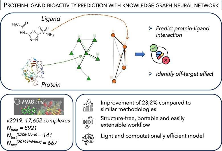
Graphical abstract
1. Introduction
Most small drug-like molecules act as ligands and bind to proteins [1], [2]. Therefore, protein–ligand interactions (PLIs) with primary and secondary pharmacological targets critically determine the efficacy and safety profile of a drug [3], [4]. Prediction, quantification, and interpretation of PLI are, therefore, integrative components of pre-clinical drug discovery [5], [6].
A plethora of experimental methods has been developed for PLI quantification, including well-established biophysical and biochemical binding assays, as well as omics-based methods, such as chemoproteomics [7]. Binding assays can be both fast and accurate for a few targets of interest [8]. However, our ability to probe proteome-wide PLIs with such assays is limited by the availability of large quantities of the purified proteins of interest [9]. In addition, quantification of proteome-wide PLIs is labour-intensive, time-consuming, and often results in only moderate sensitivity [10].
Computational methods predicting PLIs complement experimental approaches and are indispensable in drug discovery [11], [12], [13]. Some methods simulate molecular docking [14], [15], while other methods rely on structure-based representations of the protein–compound complex, taking solved structures as inputs for machine learning algorithms [16], [17], [18], [19]. The accumulation of high-quality data derived from biochemical and biophysical screening [20], along with novel algorithms, has empowered such methods. However, a significant limitation remains: only a limited number of complex structures have been solved. Consequently, screening procedures are increasingly being complemented or replaced by modelling procedures [21], [22].
A major issue associated with traditional docking-based approaches is the generation ofligand docking poses. This process is often a bottleneck because creating plausible binding conformations of protein–ligand complexes without experimental data is challenging. These challenges include accounting for the dynamic nature of proteins and ligands, which undergo conformational changes during binding. This problem is compounded by the fact that structural models must strive to implicitly capture the impact of these conformational changes accurately, a challenge noted in recent studies [23]. However, choosing not to use structural information has its downside, and could result in the loss of valuable inputs needed to understand surfaces specificities, potentially overlooking binding pockets or local charges.
Besides the limitation of structures, most existing computational methods also do not consider several biological factors that may contribute to PLI. For instance, localisation and expression of proteins are usually not considered, and most methods treat proteins as isolated entities, ignoring protein–protein interactions that are ubiquitous under physiological conditions [24]. This leaves room for new prediction algorithms that are able to circumvent existing limitations and embed additional knowledge into the prediction process. Such algorithms have the potential to improve prediction performance, and to yield a better understanding of the relative importance of individual factors.
During recent years, applications of deep learning techniques have greatly expanded in drug discovery [25]. In particular, geometric deep learning and graph neural networks (GNNs) have been widely used for molecular representations [26], structure-based drug design [27], [28], [29], [30], molecular property prediction [31], [32], [33], [34], and protein–ligand binding predictions [35], [36]. Besides their good performance in many tasks, GNNs are particularly appealing in the context of PLI prediction for two reasons. First, in contrast to traditional deep learning, geometric deep learning can operate in non-Euclidean spaces, thus it is able to capture diverse information that is not easily embedded into a Euclidean representation, such as graphs that consist of nodes and edges [37]. Thus, GNNs are able to capture complex and interdependent relationships between biological entities on multiple scales. The benefit is particularly prominent in protein-relevant tasks, such as protein representation [30], [38], [39], protein folding [40], protein design [41], [42], and protein–protein interaction [43], [44], [45], [46], [47], [48], [49]. Second, various research groups have developed new techniques to improve the interpretability of GNNs [25], [50], [51]. We also hypothesised that heterogeneous multimodal graphs are well-suited for representing entities and their interactions within real-world systems, and are therefore an ideal choice for modelling biochemical processes in a coarse-grained manner [52]. Taking into account these benefits, as well as challenges and concerns raised about the use of complex deep learning approaches [16], [53], we consider heterogeneous GNNs a natural candidate for the task of PLI prediction.
Here, we report a novel GNN model termed G–PLIP (Graph for Protein Ligand Interaction Prediction). G–PLIP quantitatively predicts PLIs using non-structural features of proteins and ligands. We demonstrate that G–PLIP performs comparably with or better than state-of-the-art structure-aware models, while the computational cost remains low, thanks to its simple model architecture and the encapsulation of the chemical sub-space into a single graph. We analyzed the contribution of individual feature types to the model's performance and demonstrated that the primary sequences of proteins, together with molecular information of ligands, contain rich information which can be exploited for PLI prediction.
2. Methods
2.1. Architecture of a heterogeneous GNN
We constructed a heterogeneous knowledge graph featuring two distinct node types N: ligands represent drugs or drug-like molecules , and proteins encompass target proteins . The graph incorporates three types of links: protein–protein links embodying physical binary interactions between proteins ; ligand–ligand links reflecting chemical similarity between compounds ; and protein–ligand links representing bioactivity between ligands and protein targets . G is undirected, therefore . The model adopts a non-linear multiconvolutional neural network with an encoder–decoder architecture: the encoder generates node embeddings via convolutional layers, and the decoder predicts bioactivities, as shown in Fig. 1.
| (1a) |
| (1b) |
1: The Jaccard Index, gauges the similarity between two sets of discrete values A and B, and is defined as the size of the intersection divided by the size of the union; and the Tanimoto Similarity Score, extends the concept to continuous values.
| (2) |
2: The GraphSAGE operator for node i, from Hamilton et al. [54]. The updated embedding of node i, denoted by , is computed as a weighted sum of its own embedding and the mean of the embeddings of its neighbours . Here, and are learnable weight matrices. The operator calculates the mean of the embeddings of the neighbours of node i.
Fig. 1.

Overview of G–PLIP. At its core, the model implements a knowledge graph derived from the protein–protein interactome and in-vitro pharmacology data (middle panel). The heterogeneous graph consists of binary protein–protein interactions and drug–drug similarities. Information is integrated into the model in the form of feature vectors of protein and molecule nodes (left panels). The highlighted network in the right panel encodes information of node P3 and C2 from their neighbours and decodes their embedding to predict the P3–C2 bioactivity (pAct).
2.1.1. Protein features
The encoder leverages three distinctive types of protein features.
-
•
kmer count: kmer counting from protein sequences endows G–PLIP with an understanding of protein characteristics. This entails tallying the occurrences of every substring of length k within a given sequence, yielding a commonly employed distance measure [55]. We hypothesised that, given the relatively modest size of drug-like molecules, it is sufficient to inspect 3-mers to consider the catalytic site and its immediate vicinity in the context of PLI prediction. Therefore, we used 3-mers as features for a total of 8000 (203) combinations, which were calculated from the protein sequence available on UniProt [56].
-
•
Subcellular location: Proteins' roles within the cellular machinery can often differ based on their location, thereby influencing their properties and giving insights about their interactions. We used information pertaining to the mature protein's location in the cell, extracted from UniProt. Subcellular locations are grouped into 31 main classes, and we employ one-hot encoding for representation.
-
•
Gene expression: The abundance of proteins, or as a proxy, that of their encoding mRNAs which can be measured by diverse sequencing techniques such as RNA-seq. Gene expression patterns have been correlated with drug effects [57], and can be adapted depending on the cell or tissue type of interest. For each protein, we incorporated normalized Transcripts Per Million (nTPM) from RNA-seq data, averaged across the corresponding expressed genes. We used gene expression data from the Human Protein Atlas [58]. Gene expression was averaged across all tissues by default, although we left this setting open to modification for more specific drug discovery applications to screen compounds interacting with specific pathways.
2.1.2. Compound features
Similarly, the encoder harnesses three distinct types of compound features, each providing a comprehensive representation of molecular attributes:
-
•Lipinski's rule of five: Aiming to evaluate druglikeness, this rule is widely used in pharmacology, assessing whether a compound possesses attributes suitable for an oral drug. The rules [59] state that, in general, an orally active drug has:
-
1.Not more than 5 hydrogen bond donors (OH and NH groups)
-
2.Not more than 10 hydrogen bond acceptors (notably N and O)
-
3.A molecular weight under 500 g/mol
-
4.An octanol-water partition coefficient (log P) that does not exceed 5
-
1.
-
•Chemical features: In order to capture the main characteristics of a compound, we also extracted the following chemical features:
-
1.Topological Polar Surface Area (Å2)
-
2.Number of rotatable bonds (#)
-
3.Molecular Refractivity (MR) [62]
-
4.Number of atoms (#)
-
5.Number of aromatic rings (#)
-
6.Number of aliphatic rings (#)
-
7.Percentage of atoms belonging to aromatic rings (%)
-
1.
-
•
Fingerprints: We generated Morgan fingerprints [63] from the SMILES representation of compounds and folded them into a bit vector. G–PLIP uses by default the extended-connectivity fingerprints (ECFP) with a diameter of 4, i.e., ECFP4. ECFPs are circular topological fingerprints designed for molecular characterisation or similarity searching, being widely employed as molecular descriptors for machine learning models [11]. Those identifiers represent substructures present within the molecule, by assigning integer identifiers to each non-hydrogen atom of the input molecule and iteratively updating them to capture larger and larger circular neighbourhoods. Those final integer identifiers can be converted to fixed-length bit strings, with the risk of collision and therefore loss of information increasing as the bit string is shorter. As neural networks can be quite sensitive to background noise, we encoded our fingerprints in a 256 bit vector [64], [65]. The size and the choice between ECFP and FCFP (Functional-Class Fingerprints [63]) of the model can be configured by the user.
With the default settings, the graph encapsulates 8032 features for the protein nodes and 267 features for the compound nodes .
2.1.3. Interaction networks
We extracted 15,749 protein–protein interactions (PPIs) between 939 human proteins from a PPI database successfully used by [52] on a similar heterogeneous graph neural network approach investigating polypharmaceutical side effects. We linked all the ligands together to form a full graph, where ligand–ligand connections symbolize compound similarities quantified by Tanimoto scores (Equation (1b)), a measure resembling the Jaccard Index (Equation (1a)). The Jaccard index measures similarity between finite sample sets and is defined as the size of the intersection divided by the size of the union of the sample sets. Likewise, the Tanimoto score (also referred as Tanimoto similarity ratio) expresses a similarity ratio over Morgan fingerprint bitmaps, defined as the number of common bits divided by the bit length. Similarity values range from 0 to 1, where 1 indicates identical molecules (accounting for potential information loss during bit encoding). Our pipeline permits customisation of ligand connectivity to consider only connections surpassing a specified Tanimoto score threshold. By default, we incorporated all compound–compound similarities (keeping the threshold to 0.0), giving a complete subgraph of compounds. It results in a graph with nodes and edges, with P representing the number of proteins, C the number of ligands and k the average degree of connectivity of proteins, defined as (since the graph is undirected) depending on the PPI database used. In the default configuration, the graph has two distinct connected components, thus we attempted to model the protein–ligand edges in one of the experiments (Table 6, reported as ‘w/ DTIs’).
Table 6.
a) G–PLIP's performances evaluated through an ablation study involving different graph topologies. ‘w/o PPI’ (i.e., protein–protein interaction) disregards protein–protein connectivity but utilizes other available features and connections. ‘w/o CompSim’ (i.e., compound similarity) does not incorporate compound–compound similarities but still integrates compound–compound connectivity (without weight on the edges). ‘w/o CompLink’ does not connect compounds at all but utilizes protein–protein connections. ‘w/o PPI & CompLink’ does not utilize either protein–protein or compound–compound connectivities. Each setup typically retains all other features and connections, and −ΔRMSE is displayed compared to the complete model. ‘w/ DTIs’ (i.e., drug–target interaction) draws drug–target interactions from the train set above every other connection mentioned, which means the encoder won't be limited to the protein or compound subgraph anymore. b) G–PLIP's performances when only using graph topologies. ‘only PPI’ utilizes only protein–protein connectivity. ‘only CompSim’ integrates compound–compound similarities. ‘only PPI & CompSim’ normally connects compounds and proteins. In all of these cases, other features are excluded, and −ΔRMSE is reported in comparison to the null model.
| (a) Graph contributions, from the complete model | ||||||||||||||||||||||||||||||||||||||||||||||||||||||
| ||||||||||||||||||||||||||||||||||||||||||||||||||||||
| (b) Graph contributions, from the null model | ||||||||||||||||||||||||||||||||||||||||||||||||||||||
| ||||||||||||||||||||||||||||||||||||||||||||||||||||||
2.2. Link predictions
The proposed GNN consists of two primary components: (a) an encoder that produces node embeddings from the original graph, and (b) a decoder that uses embedding features to forecast drug–target activities. The encoder processes an input graph and generates a d-dimensional embedding for each node, aiming to incorporate original node information. This encoder contains two distinct components: the first encapsulates proteins and binary protein interactions, while the second handles ligands and compound–compound similarities.
Both components of the encoder consist of a singular convolutional layer, updating the node features within a latent dimension using the GraphSAGE operator (Equation (2)) designed for low-dimensional embeddings of nodes in large graphs [54]. The GraphSAGE operator serves as a learnable function that generates embeddings by aggregating information from a node's local neighbourhood. As message-passing GNNs cannot be applied trivially to heterogeneous graphs, we bypass this limitation by having individual convolutional layers for each edge type. Therefore, the algorithm iterates over edge types to perform the convolution.
The decoder is composed of two linear layers, which employ concatenated embeddings of the protein target and compound molecule to predict bioactivity as a continuous value. A dropout layer is interposed between the two linear layers to prevent overfitting. Given that bioactivities are commonly expressed in a logarithmic scale (pAct, defined as -log10(Ka)), we used the Rectified Linear Unit (ReLU) activation function to rectify any negative values within the layers because such values don't align with biological meaning.
2.2.1. Model training
We formulate the task of PLI prediction as a multirelational link prediction problem in a heterogeneous graph. We subsequently trained a GNN model to predict bioactivities of unseen protein–ligand pairs (Fig. 1), using the root mean square error (RMSE) as the loss function for model training and backward propagation. We opted for a regression task, primarily due to the inherent subjectivity associated with any threshold value used to categorize ground truth data, and secondly because of the goal of identifying possible off-target effects by directly comparing bioactivities. The model possesses 8449 trainable parameters, and was trained using the Adam optimizer [66] with a learning rate of 0.001 and a batch size of 512 over 500 epochs.
We assessed different configurations using a two-sample t-test to compare the predictions of our current best setting, , with those from the new setting, . The null hypothesis () posits that the means of the two predictions are equal (), while the alternative hypothesis () asserts that the mean prediction of the new setting is greater than that of the current best setting (). We set the significance level (α) for the p-value at 0.05. Throughout this study, we provide the corresponding p-value to support any claims about the insignificance of a change.
During the design process, various configurations were tested, including different numbers and types of convolutional layers, learning rates, batch sizes, dropouts, PPI networks, compound similarity thresholds, and sizes of Morgan fingerprints (Table S3, S1a and S1b). Notably, a more complex encoder with multiple convolutional layers was tested but did not significantly improve performance (p-value = 0.626). We also attempted to use cutting-edge embeddings of protein sequences [67] and compound formulae, without observing better performance (Table S2).
| (3a) |
| (3b) |
| (3c) |
3: The Root Mean Square Error (), Pearson Correlation Coefficient () and Coefficient of Determination () evaluating the correctness of predicted values compared to the ground truth values y.
The RMSE (Equation (3a)) stands as the prevalent loss metric for regression models, and is conventionally used to assess model performances, whereas we also reported several other metrics. Commonly used, the Pearson correlation coefficient (, Equation (3b)) gauges the linear correlation between the ground truths and the predicted values. Nonetheless, its exclusive focus on correlation can yield diverse interpretations and has been a subject of concern in regression evaluation [68]. Consequently, we also reported the coefficient of determination (Equation (3c)).
Furthermore, for accurate identification of off-target activities, the ranking of predicted bioactivities in relation to one another is sometimes as important as exact predicted values, because the rankings allow prioritisation of off-target testing and generation of hypotheses for drug repurposing. In essence, identifying off-target effects provides new insight into existing drugs, unveiling their potential to treat diseases for which they were not initially designed, for instance in the case of the repurposing of the drug rapamycin [69]. Therefore, we used a new metric, Rank-Biased Overlap (RBO, defined in Equation (4)) [70], to evaluate G–PLIP's proficiency to detect the most probable off-target effects by potency. RBO is a similarity measure, used to quantify the differences between two rankings. Compared to Spearman's ρ commonly used to evaluate rankings, RBO has the advantage of being weighted, and favours the top of the ranking depending on its persistence parameter p, which was set to 0.5 for this study.
| (4) |
4: The Ranked Biased Overlap (RBO) formula for comparing the similarity between two rankings S and T of length D. and are the top-d elements of rankings S and T respectively; and the parameter p controls the steepness (or persistence) of the weighting, with lower values of p giving more weight to higher ranks, while higher values explore the ranking at a deeper depth [70].
Designed to measure similarity between nonconjoint, indefinite or incomplete ranking lists, RBO is tuneably top-weighted (parameter p) and provides a consistent way to handle tied ranks and prefix rankings of different lengths.
2.3. Datasets
2.3.1. The Roche PACE dataset
We trained the model on data derived from the Roche Pathway-Annotated Chemical Ensemble (PACE) library, an extension of the published Roche Small-molecule PAthway Research Kit (SPARK), a chemogenomic library annotated with biological pathways [71]. We leveraged the data that we collected for the PACE library to train G–PLIP, leveraging 2972 proprietary PLI measures for 2057 PACE compounds.
Since it is easier to predict the affinity of compounds that are derivatives of a well-studied pharmacophore than to make predictions for new compounds, we also performed scaffold splitting using the Bemis & Murcko (BM) scaffolds [72]. As scaffolds serve as the foundation for the subsequent exploration of derivative compounds designed and synthesized based on their structural framework, scaffold split gives a more realistic estimate of a model's performance for drug discovery purposes. We divide compounds into R-groups, linkers, and ring systems, and define a scaffold by removing all R-groups while retaining all ring systems and linkers between them. We use scaffolds to identify molecules that belong to the same chemotype and assign such molecules either to the train or test sets exclusively. This approach ensures maximal dissimilarity of train and test sets and reflects a realistic drug discovery scenario where models are applied on previously unseen scaffolds.
2.3.2. The PDBbind dataset
The PDBbind dataset, curated by Wang et al. [73], [74], presents a comprehensive collection of qualitative binding affinity data for biomolecular complexes, enriched with detailed structural information. PDBbind serves as one of the gold standards used to assess structure-based PLI models [16], [17], [18], [19], such as the popular Comparative Assessment of Scoring Functions (CASF) benchmark. The general set of PDBbind 2019 includes 17652 protein–ligand complexes, with 4852 of them being in the refined set which contains complexes with high-quality structural data. Within this database, the PDBbind Core set aims at providing a relatively small set of high-quality protein–ligand complexes for evaluation and comparison of docking/scoring methods and is notably used as the final evaluation set for the CASF competition. The latest version of this core set, used for CASF-2016, contains 285 protein–ligand complexes from 57 target proteins.
We evaluated the overlap between the PACE dataset and the PDBbind dataset. We observed that the two datasets are highly divergent, with a Jaccard index (Equation (1a)) of 0.02 between available compounds (207 compounds) and of 0.004 between known compound–target bioactivities (41 samples).
2.4. Model inference
Subsequently, we scrutinized the relative contributions of individual feature types for G–PLIP's predictions by iteratively comparing multiple instances of G–PLIP and investigated the impact of different features. Given the vast number of possible feature combinations, we restricted our experimentation to quantifying only the contributions of: (a) features in a graph; (b) subgraph connectivity with built-in features; (c) subgraph connectivity without any features; (d) usage of known drug–target interactions within the graph itself; (e) usage of different interactomes; (f) usage of different gene expressions; (g) exclusive focus on proteins or on compounds; as well as estimating the relevance of a simpler representation. We either started from a null model that uses the correct topology but does not contain any informative features and subsequently added features (Table 5, Table 6b), or started from the complete model from where we performed an ablation study by removing some of its components (Table 6a).
Table 5.
G–PLIP's performances on the PACE dataset considering different sets of features. ‘Null’ uses the graph topology but neither protein nor compound features. Indicated are the sets of features used in addition to the null model. Protein features include kmer counts (K), gene expression (GE), and subcellular localisation (SL). Compound features include fingerprints (F, for instance extended connectivity fingerprint, ECFP), Lipinski features (L) and other chemical features (Ch). −ΔRMSE represents the change in performance compared with the ‘Null’ model.
| (a) Feature contributions | ||||||||||||||||||||||||||||||||||||||||||||||||||||||||||||||||||||||||||||||||||||||||||||||||||||||||||||||||||||||||
| ||||||||||||||||||||||||||||||||||||||||||||||||||||||||||||||||||||||||||||||||||||||||||||||||||||||||||||||||||||||||
We reported the four metrics (RMSE, RBO, , and ) alongside the improvement from the null to the complete model, defined in Equation (5).
| (5) |
To distinguish the learned biochemical insights of the model from any artificial correlations learned from graph topology, we defined a null model as trained on randomly labelled edges, with bioactivities drawn from a uniform distribution between 3 and 11 (pAct values considered as extremes). To quantify stochasticity, we repeated the experiment 20 times with different random seeds and reported the averaged results as being representative of the null model.
We then tested G–PLIP on a dataset of randomly connected edges, with bioactivities shuffled alongside the known drug–target pairs from the existing data, and performed the experiment with the seed used for further tests relative to feature contributions (Table 1). This procedure aimed to distinguish potential bias stemming from the dataset curation protocol from the model's actual learning ability.
Table 1.
G–PLIP assessment on the Roche PACE dataset using different settings, depicting the difference of performances between the default stratified split, the scaffold split, and two control conditions (edge labels randomly assigned, and edge labels shuffled).
| Model | ||||
|---|---|---|---|---|
| G–PLIP - Baseline | 0.862 | 0.680 | 0.525 | 0.246 |
| G–PLIP - Scaffold Split | 0.886 | 0.660 | 0.499 | 0.208 |
| Random Edges | 1.982 | 0.111 | 0.036 | -0.015 |
| Shuffled Edges | 1.064 | 0.731 | 0.051 | -0.033 |
Notes: ↑ denotes a metric where higher is better, ↓ the reciprocal.
Finally, we investigated concerns raised by previous studies about the relevance of intricate deep learning methodologies compared to standard techniques for inferring binding affinities [16], [53], [75], [76], [77] by comparing the performance of G–PLIP to state-of-the-art machine learning models. We thus used AutoGluon, a framework encapsulating state-of-the-art techniques and automating their optimisation [78], inputting the same features to evaluate the gain of a graph neural network architecture.
3. Results
3.1. Prediction of drug–protein activity (pAct)
G–PLIP was primarily trained and evaluated on data derived from the Roche Pathway-Annotated Chemical Ensemble (PACE) library. We first performed a 80%-20% split, stratifying the split by proteins. Each of the proteins will have the same proportion of links dispatched between the train and test set, for an equal representation across the sets to guarantee a fair evaluation. Proteins possessing only one link were excluded from the split and retained for a specific use case. We then used a 80%–20% scaffold split to evaluate the model, grouping molecules derived from the same scaffold into the same set. G–PLIP produced a good accuracy in both settings (Table 1), particularly noteworthy with respect to its performances when subjected to randomized data.
We investigated the model's behaviour and observed intriguing characteristics. First, despite largely concordant predictions, the model has a propensity to underestimate high bioactivities on the Roche PACE dataset (Fig. 2, panel a), without their being subsequently observed in the PDBbind dataset (Fig. 2, panel b and c). This tendency leads to discrepancies between the performance judged by different metrics, with and scores indicating a moderate performance while indicating a good performance. Second, the model is also able to predict pAct values for missing links, i.e. cases where there is no quantitative information about the interaction between a protein and a ligand. Note that in the context of protein–ligand interaction, a missing link does not necessarily mean a lack of interaction; it may arise due to a lack of measurement, a reporting bias, due to the sensitivity of the assay, or a combination of these factors. Interestingly, the median predicted value of missing links is lower than the predicted values for non-missing links (Supplementary Figure S2). Finally, our model achieves a comparable performance for a wide range of targets classified by their molecular functions (Fig. 3 and Supplementary Figure S1).
Fig. 2.

Performance of G–PLIP with PACE and PDBbind datasets. Top panels are scatter plots of ground-truth values (y-axis) against predictions (x-axis) from the test samples. The yellow region shows the values below the mean RMSE. A fitted linear regression model prognosticating ground truths from predictions is sketched in red, with 95% confidence intervals indicated in shades. In the bottom panels, an MA plot portrays the differences between predicted values and ground truths (y-axis) against the average of the two (x-axis). The mean and two units of standard deviation of the differences are indicated by dashed lines. The trendline to visualize the bias is highlighted in red. Displayed are test samples from the Roche PACE dataset (panel a), the PDBbind 2016 CASF Core set (panel b) and the PDBbind 2019 Hold-out set (panel c).
Fig. 3.

G–PLIP's performance, trained and tested with the PACE database, stratified by molecular function classes of targets. Target classes are sorted by median RMSE values. The black vertical line is the overall mean value across all molecular function classes. Molecular functions possessing less than 10 targets are not displayed.
3.2. Comparison with state-of-the-art pipelines
Having established a baseline performance, we next evaluated G–PLIP with independent datasets and compared it with other pipelines designed for the same task on PDBbind, a collection of independent datasets curated by Wang et al. [73], [74]. We compared the performance of G–PLIP with those of state-of-the-art (SOTA) models that leverage structural information [16], [17], [18], [19], primarily by using convolutional neural networks or recurrent neural network-based approaches. In order to assess the merit of the structure-free methodology, our model only leveraged the amino-acid sequence of proteins and the SMILES representations of compounds despite the availability of structural data in the PDBbind dataset. Since our approach is grounded in human tissue gene expression data, and tailored for applications in drug discovery, we restricted the comparison to PLI of human proteins. Employing protocols established in the literature [16], [17], [18], [19], we performed a comparative study with two distinct setups and reported RMSE and , which are the metrics reported in the aforementioned references, as well as and RBO when available.
First, we assessed G–PLIP using as a test set the 2016 CASF Core Set (n = 141), a benchmark set compiled by the PDBbind team, with the remaining database entries constituting the training set (n = 8921). Subsequently, we evaluated G–PLIP by a temporal splitting of the PDBbind dataset (denoted as the 2019 Hold-out Set), where the 2016 version serves as a training set, while the samples introduced in the 2019 and 2020 versions were utilized to test the model (n = 667). We further partitioned the training data into training and validation subsets, with the latter aiding in the selection of the optimal model across hyperparameters. Yuel [79] and Pafnucy [17] were retrained and assessed using the same train/test split, while [19], Fusion [18] and IChem–PLI [16] were obtained from the original publications.
G–PLIP outperformed its peers on the external 2016 CASF Core Set judging by RMSE, as shown in Table 2, with an improvement of 21.5% compared to Yuel [79], 19.4% compared to [19], 21.8% compared to Fusion [18], 30.0% compared to Pafnucy [17] and 32.3% compared to the most complete IChem model (with merged protein, ligand and interaction graph, namely IChem–PLI) [16]. On the 2019 Hold-out set, G–PLIP performs better by 31.7% compared to , 27.3% compared to Fusion, 25.1% compared to Pafnucy [17] and 34.3% compared to the IChem–PLI model, yet 4.8% worse than Yuel. Overall, we observed a propensity for complex models to overfit to the biases present in the temporal split (2019 Hold-out Set).
Table 2.
Performances of G–PLIP on the PDBbind dataset over ten independent trainings (reported as mean ± sd), and comparison with state-of-the-art models over two different splits (2016 CASF Core Set and 2019 Holdout Set). Results for Yuel [79] and for Pafnucy [17] were manually compiled from a model retrained locally using the parameters proposed by the authors on the same train/test splits. We also reported baselines claimed in previous studies, indicated with a star (*): KDEEP according to the performances claimed in the original paper [19] (for the 2016 Core Set) and manually investigated by a later study [18] (for the 2019 Hold-out Set); Fusion according to the best performances reached during the study, namely by the midlevel fusion[18]; Pafnucy [17] and IChem–PLI as obtained from the original IChem–PLI paper [16].
| (a) Comparison with SOTA models on the PDBbind 2016 Core Set, used as final benchmark for the Comparative Assessment of Scoring Functions (CASF) competition. | |||||||||||||||||||||||||||||||||||||||||||||||||
| |||||||||||||||||||||||||||||||||||||||||||||||||
| (b) Comparison with SOTA models on the PDBbind 2019 Hold-out Set, from a temporal split. | |||||||||||||||||||||||||||||||||||||||||||||||||
| |||||||||||||||||||||||||||||||||||||||||||||||||
As the comparison was confined to PLIs of human proteins, the results for Pafnucy on the Hold-out set showed a clear improvement compared to those reported in the IChem–PLI paper [16]. Interestingly, Pafnucy's performance on the 2016 CASF Core Set is consistent with previously reported results, which bolsters confidence in the comparison with other reported baselines. In both cases, we did not observe the tendency to underestimate high-affinity interactions, as seen in the PACE dataset (Fig. 2, panel b and c). To ensure the consistency of the model's performance, we conducted ten distinct training runs and reported the mean performance with its standard deviation (SD), confirming its reliability.
Pearson correlation coefficients are reported to be slightly lower for G–PLIP on the core set. However it has been shown this metric can be deceptive when evaluating predictive performances on regression tasks [68], and it is highly sensitive to extreme outliers and influenced by the range of observations [80]. In consequence, satisfactory Pearson correlation coefficients could be obtained using models unable to predict relevant values, and this hypothesis was corroborated by training a model using the aforementioned correlation coefficient as a loss function. It yielded a Pearson correlation coefficient of 0.79 while proposing a RMSE of 6.12, and thus does not offer any practical predictive power (Supplementary Figure S4). We also attempted transfer learning by training a model on the PACE dataset and evaluating it on the PDBbind Core and Hold-out test sets. The performance, however, was significantly worse than that obtained from the model trained on the PDBbind dataset.
3.3. Contribution of low-quality data to improve G–PLIP 's learning abilities
Previous studies are inconclusive about whether extending datasets by integrating low-quality affinity data enhances the performance of machine learning models. While some studies demonstrated improvements in this context [81], recent investigations have posited that such integration exerts minimal [19] or even misleading influence on model outcomes [76], [82], [83]. PDBbind's general dataset is proposed with a subset curated by the authors, the refined set, containing data considered as being especially qualitative. To address this discrepancy, we conducted experiments using distinct subsets from the PDBbind collection: the complete, refined, and other sets. The complete set represents the entire PDBbind dataset, the refined set encompasses a subset of high-quality data curated by the authors, and the other set comprises the data not present in the refined subset.
Each of these three sets was employed for training and subsequently evaluated on both the 2016 CASF Core Set and the 2019 Hold-Out Set, following the same protocol as previously described. The first setup provides a consistent benchmark using reliable test samples carefully selected and segregated from the three subsets (141 bioactivity values). In the second setup, we aimed to gauge the model's ability to generalize within the given subset. Here, the test data's composition directly mirrors the training subset's characteristics, enabling us to observe the model's behaviour when trained and evaluated on data of similar quality.
Results in Table 3 indicate that augmenting the dataset with lower-quality samples confers little benefit to the model's performance. Indeed, when evaluating the model on an external reference set (CASF-2016 Core), the results achieved on the complete set are only slightly better than those on the refined subset. Additionally, the model trained on the other subset fails to reach their baseline performances, despite demonstrating favourable metrics on the hold-out set. The model's performances displayed from the temporal split appear to be influenced by other factors, possibly including the narrower distribution of bioactivity values.
Table 3.
Performances of G–PLIP on the full set and two subsets of the PDBbind dataset over ten independent trainings (reported as mean ± sd). The 2016 CASF Core Set is external and thus constant over the subsets, while the 2019 Holdout Set is done by temporal splitting over the selected subset and thus dependent of its content.
| Model | 2016 Core Set |
2019 Hold-out Set |
||
|---|---|---|---|---|
| Complete | 1.023 ± 0.022 | 0.783 ± 0.007 | 0.973 ± 0.009 | 0.671 ± 0.006 |
| Refined | 1.146 ± 0.020 | 0.722 ± 0.013 | 1.102 ± 0.009 | 0.744 ± 0.010 |
| Other | 1.437 ± 0.012 | 0.690 ± 0.000 | 0.995 ± 0.011 | 0.596 ± 0.008 |
3.4. Contributions of graph features
We assessed the performance of a series of partial versions of the model using combinatorial subsets of features. We started from the null model, a configuration encompassing protein–protein interactions and drug–drug similarities but without any specific node features. We then gradually added sets of protein or compound features to the null model. In each configuration, we documented the optimal performance achieved, thereby facilitating an exploration of the contributions of individual features and their impact on enhancing predictive capacity.
According to the results (Table 5), kmer counts is the most pivotal feature, yielding a substantial improvement of RMSE by 14.08% compared to the null model. Two other protein features, gene expression and sub-cellular localisation, do not noticeably improve the prediction beyond the capability of kmers.
We observed that protein node features emerge as more informative than their compound counterparts. As we suspected, molecular fingerprints improved the prediction. We also expected that neither the features derived from Lipinski rules, nor other chemical features commonly used to roughly gauge physico–chemical properties of the molecules, would be greatly informative since they reflect rather on the pharmacokinetic properties and drug-likeliness of the molecules rather than bioactivity.
Considering that kmer was the most prominent feature that we identified, we attempted to extend or substitute kmer counts with ESM2 [67], a state-of-the-art embedding of proteins derived from evolutionary modelling. Yet we observed no discernible performance improvements (Table S2), and the simplicity coupled with the good performance recommend kmer as an informative feature for any PLI prediction algorithm.
Another intriguing finding is that the model shows remarkably good performance even in the absence of protein–protein or compound–compound connectivity (Table 6). It's essential to clarify that in such models, despite the absence of connections, the graph structure is used implicitly. This is because the encoder remains a key component of the model, and it is responsible for embedding the initial set of node features into a lower dimensional space. In addition, leaving out protein–protein and compound–compound connectivity leads to a small reduction in the performance. Nevertheless, we consider the observation interesting and worth reporting, because it underlies the power of GNNs to dissect relative contributions from node and edge features. Our attempt to model the protein–ligand interactions from the training set directly in the graph topology (referred as “w/ DTIs”) did not lead to any significant improvement of performances (p-value = 0.097), and this suggests that the model is being biased by only seeing a limited subset of possible interactions.
4. Discussion
4.1. Learning capabilities of the model
When assessed in terms of RMSE, our structure-free approach compares favourably with advanced cutting-edge structure-aware models like IChem–PLI, Pafnucy, or Fusion, as well as with novel structure-free models such as Yuel.
Our evaluation highlights the importance of choosing an appropriate metric for benchmarking studies for the task of PLI prediction. As previously mentioned, the Pearson correlation coefficient can be misleading in evaluating regressive models, and we established that satisfactory scores can be achieved even by models incapable of predicting relevant values (Supplementary Figure S4).
G–PLIP offers a new scheme for making structure-free predictions of protein–ligand interactions with a graph-based architecture. In docking-based approaches, the generation of poses is often one of the biggest bottlenecks, as it is challenging to generate plausible binding conformations of protein–ligand complexes without any experimental data. Our observations are consistent with recent studies discussing consistent conformational changes during drug-binding process [23], a challenge that current structural models are still striving to address.
The knowledge graph structure inherent to our methodology encapsulates informative protein and compound embeddings, obviating the need for an excessively complex model architecture. In this work, we only included a basic set of features in order to achieve a minimal and parsimonious model structure. Further work can build upon our model to include more information thanks to the open and adaptive framework provided by GNNs.
The minimalistic architecture of G–PLIP, with only 8,449 trainable parameters, facilitates training on non-professional computing units without any high-end GPU and is robust to overfitting. In comparison, Yuel [79], the sole structure-free method tackling the same task that we are aware of, comprises 1,411,523 trainable parameters.
4.2. Inference of the model
G–PLIP exhibits remarkable learning capabilities even in the absence of protein–protein or compound–compound connectivity, with the encoder layers being used to encapsulate the original features within a low-dimensional space without any convolutional mechanisms or aggregation. Regardless of the PPI database employed, and whether the PPI depicts physically interacting pairs only or a mix of functional and physical interactions, the protein–protein connectivity seems to make a limited contribution to the prediction. These observations, coupled with measures of node feature contributions, suggest that the information aggregated from neighbouring nodes is currently not being effectively utilized by the model. One may wonder whether alternative designs of convolutional layers might better aggregate information from a biological knowledge graph. After all, previous studies suggest that deep learning neural networks have not fully exploited their learning potential [53]. A further explanation could be found in the inherent shortcomings of the existing protein–protein interaction networks, particularly in their high rates of false positives and false negatives [84], and different PPI databases could be probed in this regard [85], [86]. We think that the protein–protein interaction is only one facet within a broader spectrum of relationships that a graph can depict. Other elements such as structural similarities, folding resemblance, or evolutionary distances could be explored with the architecture that we proposed.
Our GNN approach demonstrates its suitability for the task compared to standard machine learning models in regards to RMSE (Supp Table S1c). We therefore establish the graph architecture as an expressive framework capable of embedding a wide array of biological information. In other words, our work demonstrates that GNNs are able to identify parsimonious models for a prediction task at hand. In line with this, we found that a restricted model using only kmer and molecular fingerprints exhibits performances only slightly behind the complete model (4.7% worse, see Table 4). This also shows that our implemented features motivated by drug discovery purposes, namely gene expression (regardless of the tissue choice) and sub-cellular localisation, offered a negligible contribution to the predictions. However, these results should be investigated further, as we did not conduct experiments that are able to completely characterise the impact of individual features. While the trials with ESM2 did not yield improvements, standard protein and compound representations could still potentially be substituted by more advanced representation models (Table S2), for instance those leveraged by algorithms aiming at molecular property prediction [87] or by protein language models tailored to capture specific characteristics such as coevolution [88], [89] or multiple sequence alignment-free embeddings [90].
Table 4.
G–PLIP's performance on the PACE dataset through an ablation study examining various model variants. The ‘Complete’ model utilizes all available features and the entire graph topology. The ‘Compound-focused’ model was ablated of kmer counts, gene expression, subcellular localisation, and the PPI network. The ‘Protein-focused’ model was ablated of fingerprints, Lipinski features, other chemical features, and the compound similarity network. The ‘only kmer & Fingerprints’ model retained only kmer and fingerprints, with all other features ablated. −ΔRMSE represents the change in performance compared with the ‘Complete’ model.
| Models | RMSE | −ΔRMSE | RBO | Rp | R2 |
|---|---|---|---|---|---|
| Compound-focused | 0.956 | -11.4% | 0.661 | 0.377 | 0.122 |
| Protein-focused | 0.914 | -6.5% | 0.598 | 0.444 | 0.161 |
| only kmer & Fingerprints | 0.898 | -4.7% | 0.672 | 0.493 | 0.172 |
| Complete | 0.858 | (ref) | 0.676 | 0.525 | 0.251 |
Our observation of the limited value of including lower-quality data confirms the observations of previous studies [19], [82], [83]. Integrating data from biased or untidy biochemical assays carries a risk, even when performances on the dataset split initially appears promising. Evaluations on traditional random or temporal split can extend the biases of the original set. This underscores the necessity of systematic cross-validation against an external reference test set (in our case, the CASF 2016 Core set, remaining constant over the experiments).
4.3. Limitations
Biologically, G–PLIP performed comparably well across molecular function classes (Fig. 3). The findings partially reflect the historical focus and current practice of small-molecule drug discovery. The relatively better performance for kinases, ion channels, and G protein-coupled receptors (GPCRs), may derive from the fact that many small molecules are discovered with such proteins as targets [91], and that they also comprise a large body of secondary pharmacological targets [92]. On the other hand, some transcription factors (DNA-binding) are known to be challenging targets for small molecules [93]. The relatively variable performance of our model for multiple drug classes such as transcription factors, human hydrolases, and human proteases calls for alternative modelling strategies.
Methodologically, despite improved performances compared with recent models, G–PLIP occasionally demonstrates a propensity to underestimate potent bioactivities (Fig. 2a), which remains critical for the identification of putative interactions to be explored by drug discovery projects. Future work may explore ways to further improve G–PLIP's performance, for instance performing pre-training on different properties (e.g. solubility measures).
Despite our effort to investigate relative contributions of feature types, the interpretability of G–PLIP remains limited. Further analysis can be conducted to exploit the capability and limitations of the model. We may adopt a biology-informed split strategy, for instance splitting target proteins with hierarchical clustering, using pairwise structural and sequence homology of the proteins as distance metrics. We could also examine activity cliffs and their impacts on prediction, or scrutinize protein–ligand complexes leading to outlier predictions in order to devise improvement strategies.
Computationally, modelling PLI with a knowledge graph bears a significant memory cost. It may be mitigated by refactoring the data structure or by fine-tuning the compound similarity edges. These adjustments may improve memory efficiency and scalability.
5. Conclusion
Quantitatively predicting protein–ligand interactions is an unsolved challenge at the heart of small-molecule drug discovery. Here we present a structure-free approach that exhibits enhanced predictive accuracy compared to existing methods. Moreover, we show that biochemical information can be effectively encapsulated and utilized by a deep learning procedure. Our methodology only requires an amino-acid sequence of proteins and SMILES representation of ligands, making it easily applicable without the need for prior binding poses or protein structures. Despite its simplicity, G–PLIP exhibits remarkable learning and predictive capabilities. We demonstrate that G–PLIP can efficiently be trained from a relatively small qualitative dataset and yet proficiently extrapolates to unseen interactions from learned parameters. Composed of only a few layers, the model is swiftly trainable on non-specialized platforms, and its computational performance positions it as a suitable candidate for large-scale retraining or high-throughput screening of large compound libraries. Without the need for structural data, G–PLIP can seamlessly be integrated into a de novo protein design workflow.
6. Code availability and resource requirement
A reference implementation of G–PLIP platform, based on PyTorch [94] and PyTorch Geometric [95], is available at https://github.com/simoncrouzet/g-plip.
G–PLIP was trained with 16 cores of a Xeon-Gold CPU running at 2.1 GHz, with at least 64 GB available RAM. It takes approximately 2,670 minutes to train G–PLIP on the PDBbind complete dataset, leading to a carbon footprint of 1.84 kg eq.
CRediT authorship contribution statement
Simon J. Crouzet: Writing – review & editing, Writing – original draft, Visualization, Software, Methodology, Formal analysis, Data curation, Conceptualization. Anja Maria Lieberherr: Writing – review & editing, Software, Formal analysis, Data curation. Kenneth Atz: Writing – review & editing, Validation, Formal analysis. Tobias Nilsson: Writing – review & editing, Resources. Lisa Sach-Peltason: Writing – review & editing, Validation, Resources. Alex T. Müller: Writing – review & editing, Validation, Resources. Matteo Dal Peraro: Writing – review & editing. Jitao David Zhang: Writing – review & editing, Writing – original draft, Supervision, Investigation, Funding acquisition, Formal analysis, Conceptualization.
Declaration of Competing Interest
The authors declare the following financial interests/personal relationships which may be considered as potential competing interests: Jitao David Zhang, Simon J. Crouzet, Anja Maria Lieberherr, Kenneth Atz, Tobias Nilsson, Lisa Sach- Peltason and Alex T. Müller report financial support, administrative support and article publishing charges were provided by F. Hoffmann-La Roche Ltd. Jitao David Zhang, Kenneth Atz, Tobias Nilsson, Lisa Sach-Peltason, Alex T. Müller report being currently employed by F Hoffmann-La Roche Ltd. If there are other authors, they declare that they have no known competing financial interests or personal relationships that could have appeared to influence the work reported in this paper.
Acknowledgements
This work has been conducted under the sponsorship of the internship program “Think Tank in Innovation and Sustainability #IP2TIS” initiated by André Hoffman, vice-chairman of the board of Roche Holding Ltd, and organized by Volker Herdtweck and colleagues, as well as the sponsorship of the Roche Advanced Analytics Network (RAAN). We thank Leo Klarner for esteemed discussions, Julian Shillcock for helpful comments on the language, alongside Nicolas Frey, Torsten Schindler, Francesco Brizzi and Christian Kramer for their valuable feedback, and colleagues from the Predictive Modelling and Data Analytics (PMDA) chapter of Pharmaceutical Sciences for their continuous support.
Footnotes
Supplementary material related to this article can be found online at https://doi.org/10.1016/j.csbj.2024.06.029.
Contributor Information
Simon J. Crouzet, Email: simon.crouzet@epfl.ch.
Jitao David Zhang, Email: jitao_david.zhang@roche.com.
Appendix A. Supplementary material
The following is the Supplementary material related to this article.
Supplementary materials, including additional tables of feature contributions and benchmarks, and data analysis of model output.
References
- 1.Karplus M., McCammon J.A. Molecular dynamics simulations of biomolecules. Nat Struct Biol. 2002;9:646–652. doi: 10.1038/nsb0902-646. [DOI] [PubMed] [Google Scholar]
- 2.Bissantz C., Kuhn B., Stahl M. A medicinal chemist's guide to molecular interactions. J Med Chem. 2010;53:5061–5084. doi: 10.1021/jm100112j. [DOI] [PMC free article] [PubMed] [Google Scholar]
- 3.Nicolaou C.A., Brown N. Multi-objective optimization methods in drug design. Drug Discov Today, Technol. 2013;10:e427–e435. doi: 10.1016/j.ddtec.2013.02.001. [DOI] [PubMed] [Google Scholar]
- 4.Lipinski C., Hopkins A. Navigating chemical space for biology and medicine. Nature. 2004;432:855–861. doi: 10.1038/nature03193. [DOI] [PubMed] [Google Scholar]
- 5.Jiménez-Luna J., Grisoni F., Schneider G. Drug discovery with explainable artificial intelligence. Nat Mach Intell. 2020;2:573–584. [Google Scholar]
- 6.Schneider P., et al. Rethinking drug design in the artificial intelligence era. Nat Rev Drug Discov. 2020;19:353–364. doi: 10.1038/s41573-019-0050-3. [DOI] [PubMed] [Google Scholar]
- 7.Algar W.R., Hildebrandt N., Vogel S.S., Medintz I.L. FRET as a biomolecular research tool - understanding its potential while avoiding pitfalls. Nat Methods. 2019;16:815–829. doi: 10.1038/s41592-019-0530-8. [DOI] [PubMed] [Google Scholar]
- 8.Huang L., Zhang C. Microscale thermophoresis (MST) to detect the interaction between purified protein and small molecule. Methods Mol Biol. 2021;2213:187–193. doi: 10.1007/978-1-0716-0954-5_17. [DOI] [PubMed] [Google Scholar]
- 9.Kaur U., et al. Proteome-wide structural biology: an emerging field for the structural analysis of proteins on the proteomic scale. J Proteome Res. 2018;17:3614–3627. doi: 10.1021/acs.jproteome.8b00341. [DOI] [PMC free article] [PubMed] [Google Scholar]
- 10.Backus K.M., et al. Proteome-wide covalent ligand discovery in native biological systems. Nature. 2016;534:570–574. doi: 10.1038/nature18002. [DOI] [PMC free article] [PubMed] [Google Scholar]
- 11.Carracedo-Reboredo P., et al. A review on machine learning approaches and trends in drug discovery. Comput Struct Biotechnol J. 2021;19:4538–4558. doi: 10.1016/j.csbj.2021.08.011. [DOI] [PMC free article] [PubMed] [Google Scholar]
- 12.Qin T., Zhu Z., Wang X.S., Xia J., Wu S. Computational representations of protein–ligand interfaces for structure-based virtual screening. Expert Opin Drug Discov. 2021;16:1175–1192. doi: 10.1080/17460441.2021.1929921. [DOI] [PubMed] [Google Scholar]
- 13.Romano J.D., Tatonetti N.P. Informatics and computational methods in natural product drug discovery: a review and perspectives. Front Genet. 2019;10 doi: 10.3389/fgene.2019.00368. [DOI] [PMC free article] [PubMed] [Google Scholar]
- 14.Van Zundert G.C.P., et al. The HADDOCK2.2 web server: user-friendly integrative modeling of biomolecular complexes. J Mol Biol Comput Res Mol Biol. 2016;428:720–725. doi: 10.1016/j.jmb.2015.09.014. [DOI] [PubMed] [Google Scholar]
- 15.Honorato R.V., et al. Structural biology in the clouds: the WeNMR-EOSC ecosystem. Front Mol Biosci. 2021;8 doi: 10.3389/fmolb.2021.729513. [DOI] [PMC free article] [PubMed] [Google Scholar]
- 16.Volkov M., et al. On the frustration to predict binding affinities from protein–ligand structures with deep neural networks. J Med Chem. 2022;65:7946–7958. doi: 10.1021/acs.jmedchem.2c00487. [DOI] [PubMed] [Google Scholar]
- 17.Stepniewska-Dziubinska M.M., Zielenkiewicz P., Siedlecki P. Development and evaluation of a deep learning model for protein–ligand binding affinity prediction. Bioinformatics. 2018;34:3666–3674. doi: 10.1093/bioinformatics/bty374. [DOI] [PMC free article] [PubMed] [Google Scholar]
- 18.Jones D., et al. Improved protein–ligand binding affinity prediction with structure-based deep fusion inference. J Chem Inf Model. 2021;61:1583–1592. doi: 10.1021/acs.jcim.0c01306. [DOI] [PubMed] [Google Scholar]
- 19.Jiménez J., Škalič M., Martínez-Rosell G., De Fabritiis G. KDEEP: protein–ligand absolute binding affinity prediction via 3D-convolutional neural networks. J Chem Inf Model. 2018;58:287–296. doi: 10.1021/acs.jcim.7b00650. [DOI] [PubMed] [Google Scholar]
- 20.Sutherland J.J., Yonchev D., Fekete A., Urban L. A preclinical secondary pharmacology resource illuminates target-adverse drug reaction associations of marketed drugs. Nat Commun. 2023;14:4323. doi: 10.1038/s41467-023-40064-9. [DOI] [PMC free article] [PubMed] [Google Scholar]
- 21.Di Lascio E., Gerebtzoff G., Rodríguez-Pérez, Systematic R. Evaluation of local and global machine learning models for the prediction of ADME properties. Mol Pharm. 2023;20:1758–1767. doi: 10.1021/acs.molpharmaceut.2c00962. [DOI] [PubMed] [Google Scholar]
- 22.Melnikov F., Anger L.T., Hasselgren C. Toward quantitative models in safety assessment: a case study to show impact of dose–response inference on hERG inhibition models. Int J Mol Sci. 2023;24:635. doi: 10.3390/ijms24010635. [DOI] [PMC free article] [PubMed] [Google Scholar]
- 23.Ayaz P., et al. Structural mechanism of a drug-binding process involving a large conformational change of the protein target. Nat Commun. 2023;14:1885. doi: 10.1038/s41467-023-36956-5. [DOI] [PMC free article] [PubMed] [Google Scholar]
- 24.Zhang J.D., Wiemann S. KEGGgraph: a graph approach to KEGG PATHWAY in R and bioconductor. Bioinformatics. 2009;25:1470–1471. doi: 10.1093/bioinformatics/btp167. [DOI] [PMC free article] [PubMed] [Google Scholar]
- 25.Jiménez-Luna J., Grisoni F., Weskamp N., Schneider G. Artificial intelligence in drug discovery: recent advances and future perspectives. Expert Opin Drug Discov. 2021;16:949–959. doi: 10.1080/17460441.2021.1909567. [DOI] [PubMed] [Google Scholar]
- 26.Atz K., Grisoni F., Schneider G. Geometric deep learning on molecular representations. Nat Mach Intell. 2021;3:1023–1032. [Google Scholar]
- 27.Isert C., Atz K., Schneider G. Structure-based drug design with geometric deep learning. Curr Opin Struct Biol. 2023;79 doi: 10.1016/j.sbi.2023.102548. [DOI] [PubMed] [Google Scholar]
- 28.Schneuing A., Du Y., Harris C., Jamasb A., Igashov I., Du W., Blundell T., Lió P., Gomes C., Welling M., Bronstein M., Correia B. Machine Learning for Structural Biology Workshop at the 36th conference on neural information processing systems (NeurIPS) 2022. Structure-based drug design with equivariant diffusion models. [Google Scholar]
- 29.Luo S., Guan J., Ma J., Peng J. 35th conference on neural information processing systems (NeurIPS) 2021. A 3D generative model for structure-based drug design. [Google Scholar]
- 30.Peng X., et al. Proceedings of the 39th international conference on machine learning (ICML) vol. 162. 2022. Pocket2Mol: efficient molecular sampling based on 3D protein pockets; pp. 17644–17655. [Google Scholar]
- 31.Atz K., Isert C., Böcker M.N., Jiménez-Luna J., Schneider G. Δ-quantum machine-learning for medicinal chemistry. Phys Chem Phys. 2022;24:10775–10783. doi: 10.1039/d2cp00834c. [DOI] [PMC free article] [PubMed] [Google Scholar]
- 32.Isert C., Kromann J.C., Stiefl N., Schneider G., Lewis R.A. Machine learning for fast, quantum mechanics-based approximation of drug lipophilicity. ACS Omega. 2023;8:2046–2056. doi: 10.1021/acsomega.2c05607. [DOI] [PMC free article] [PubMed] [Google Scholar]
- 33.Satorras V.G., Hoogeboom E., Welling M. Proceedings of the 38th international conference on machine learning (ICML) 2021. E (n) equivariant graph neural networks; pp. 9323–9332. [Google Scholar]
- 34.Withnall M., Lindelöf E., Engkvist O., Chen H. Building attention and edge message passing neural networks for bioactivity and physical–chemical property prediction. J Cheminform. 2020;12(1) doi: 10.1186/s13321-019-0407-y. [DOI] [PMC free article] [PubMed] [Google Scholar]
- 35.Liu X., Luo Y., Song S., Peng J. Pre-training of graph neural network for modeling effects of mutations on protein-protein binding affinity. PLoS Comput Biol. 2021;17 doi: 10.1371/journal.pcbi.1009284. [DOI] [PMC free article] [PubMed] [Google Scholar]
- 36.Wei B., Zhang Y., Gong X. DeepLPI: a novel deep learning-based model for protein–ligand interaction prediction for drug repurposing. Sci Rep. 2022;12 doi: 10.1038/s41598-022-23014-1. [DOI] [PMC free article] [PubMed] [Google Scholar]
- 37.Bronstein M.M., Bruna J., LeCun Y., Szlam A., Vandergheynst P. Geometric deep learning: going beyond Euclidean data. IEEE Signal Process Mag. 2017;34:18–42. [Google Scholar]
- 38.Zhang Z., et al. The eleventh international conference on learning representations. 2023. Protein representation learning by geometric structure pretraining. [Google Scholar]
- 39.Ingraham J., Garg V.K., Barzilay R., Jaakkola T. Proceedings of the 33rd international conference on neural information processing systems. vol. 1417. 2019. pp. 15820–15831. [Google Scholar]
- 40.Stärk H., Ganea O., Pattanaik L., Barzilay D., Jaakkola T. EquiBind: geometric deep learning for drug binding structure prediction in proceedings of the 39th international conference on machine learning. ICML. 2022;162:20503–20521. [Google Scholar]
- 41.Rudden L.S.P., Hijazi M., Barth P. Deep learning approaches for conformational flexibility and switching properties in protein design. Front Mol Biosci. 2022;9 doi: 10.3389/fmolb.2022.928534. [DOI] [PMC free article] [PubMed] [Google Scholar]
- 42.Krapp L.F., Meireles F.A., Abriata L.A., Dal Peraro M. Context-aware geometric deep learning for protein sequence design. bioRxiv. 2023 doi: 10.1038/s41467-024-50571-y. [DOI] [PMC free article] [PubMed] [Google Scholar]
- 43.Mohseni Behbahani Y., Crouzet S., Laine E., Carbone A. Deep local analysis evaluates protein docking conformations with locally oriented cubes. Bioinformatics. 2022;38:4505–4512. doi: 10.1093/bioinformatics/btac551. [DOI] [PMC free article] [PubMed] [Google Scholar]
- 44.Mohseni Behbahani Y., Laine E., Carbone A. Deep local analysis deconstructs protein–protein interfaces and accurately estimates binding affinity changes upon mutation. Bioinformatics. 2023;39 doi: 10.1093/bioinformatics/btad231. i544–i552. [DOI] [PMC free article] [PubMed] [Google Scholar]
- 45.Gainza P., et al. Deciphering interaction fingerprints from protein molecular surfaces using geometric deep learning. Nat Methods. 2020;17:184–192. doi: 10.1038/s41592-019-0666-6. [DOI] [PubMed] [Google Scholar]
- 46.Zeng M., et al. Protein-protein interaction site prediction through combining local and global features with deep neural networks. Bioinformatics. 2020;36:1114–1120. doi: 10.1093/bioinformatics/btz699. [DOI] [PubMed] [Google Scholar]
- 47.Hashemifar S., Neyshabur B., Khan A.A., Xu J. Predicting protein–protein interactions through sequence-based deep learning. Bioinformatics. 2018;34 doi: 10.1093/bioinformatics/bty573. i802–i810. [DOI] [PMC free article] [PubMed] [Google Scholar]
- 48.Krapp L.F., Abriata L.A., Cortés Rodriguez F., Dal Peraro M. PeSTo: parameter-free geometric deep learning for accurate prediction of protein binding interfaces. Nat Commun. 2023;14:2175. doi: 10.1038/s41467-023-37701-8. [DOI] [PMC free article] [PubMed] [Google Scholar]
- 49.Singh R., Devkota K., Sledzieski S., Berger B., Cowen L. Topsy-Turvy: integrating a global view into sequence-based PPI prediction. Bioinformatics. 2022;38 doi: 10.1093/bioinformatics/btac258. i264–i272. [DOI] [PMC free article] [PubMed] [Google Scholar]
- 50.Tan X., et al. Current advances and limitations of deep learning in anticancer drug sensitivity prediction. Curr Top Med Chem. 2020;20:1858–1867. doi: 10.2174/1568026620666200710101307. [DOI] [PubMed] [Google Scholar]
- 51.Vamathevan J., et al. Applications of machine learning in drug discovery and development. Nat Rev Drug Discov. 2019;18:463–477. doi: 10.1038/s41573-019-0024-5. [DOI] [PMC free article] [PubMed] [Google Scholar]
- 52.Zitnik M., Agrawal M., Leskovec J. Modeling polypharmacy side effects with graph convolutional networks. Bioinformatics. 2018;34 doi: 10.1093/bioinformatics/bty294. i457–i466. [DOI] [PMC free article] [PubMed] [Google Scholar]
- 53.Janela T., Bajorath J. Simple nearest-neighbour analysis meets the accuracy of compound potency predictions using complex machine learning models. Nat Mach Intell. 2022:1–10. [Google Scholar]
- 54.Hamilton W.L., Ying R., Leskovec J. Proceedings of the 31st international conference on neural information processing systems (NeurIPS) 2017. Inductive representation learning on large graphs; pp. 1025–1035. [Google Scholar]
- 55.Edgar R.C. MUSCLE: a multiple sequence alignment method with reduced time and space complexity. BMC Bioinform. 2004;5:113. doi: 10.1186/1471-2105-5-113. [DOI] [PMC free article] [PubMed] [Google Scholar]
- 56.The UniProt Consortium UniProt: the universal protein knowledgebase in 2023. Nucleic Acids Res. 2023;51:D523–D531. doi: 10.1093/nar/gkac1052. [DOI] [PMC free article] [PubMed] [Google Scholar]
- 57.Evans W.E., Guy R.K. Gene expression as a drug discovery tool. Nat Genet. 2004;36:214–215. doi: 10.1038/ng0304-214. [DOI] [PubMed] [Google Scholar]
- 58.Karlsson M., et al. A single-cell type transcriptomics map of human tissues. Sci Adv. 2021;7 doi: 10.1126/sciadv.abh2169. [DOI] [PMC free article] [PubMed] [Google Scholar]
- 59.Lipinski C.A., Lombardo F., Dominy B.W., Feeney P.J. Experimental and computational approaches to estimate solubility and permeability in drug discovery and development settings. Adv Drug Deliv Rev. 2001;46:3–26. doi: 10.1016/s0169-409x(00)00129-0. [DOI] [PubMed] [Google Scholar]
- 60.Shultz M.D. Two decades under the influence of the rule of five and the changing properties of approved oral drugs. J Med Chem. 2019;62:1701–1714. doi: 10.1021/acs.jmedchem.8b00686. [DOI] [PubMed] [Google Scholar]
- 61.Cui Y., et al. A bidirectional permeability assay for beyond rule of 5 compounds. Pharmaceutics. 2021;13:1146. doi: 10.3390/pharmaceutics13081146. [DOI] [PMC free article] [PubMed] [Google Scholar]
- 62.Wildman S.A., Crippen G.M. Prediction of physicochemical parameters by atomic contributions. J Chem Inf Comput Sci. 1999;39:868–873. [Google Scholar]
- 63.Rogers D., Hahn M. Extended-connectivity fingerprints. J Chem Inf Model. 2010;50:742–754. doi: 10.1021/ci100050t. [DOI] [PubMed] [Google Scholar]
- 64.Fassio A.V., et al. Prioritizing virtual screening with interpretable interaction fingerprints. J Chem Inf Model. 2022;62:4300–4318. doi: 10.1021/acs.jcim.2c00695. [DOI] [PubMed] [Google Scholar]
- 65.Wei Y., Li W., Du T., Hong Z., Lin J. Targeting HIV/HCV coinfection using a machine learning-based multiple quantitative structure-activity relationships (multiple QSAR) method. Int J Mol Sci. 2019;20:3572. doi: 10.3390/ijms20143572. [DOI] [PMC free article] [PubMed] [Google Scholar]
- 66.Kingma D.P., Ba J. 3rd international conference on learning representations (ICLR) 2015. Adam: a Method for Stochastic Optimization. [Google Scholar]
- 67.Lin Z., et al. Evolutionary-scale prediction of atomic-level protein structure with a language model. Science. 2023;379:1123–1130. doi: 10.1126/science.ade2574. [DOI] [PubMed] [Google Scholar]
- 68.Waldmann P. On the use of the Pearson correlation coefficient for model evaluation in genome-wide prediction. Front Genet. 2019;10 doi: 10.3389/fgene.2019.00899. [DOI] [PMC free article] [PubMed] [Google Scholar]
- 69.Palve V., Liao Y., Remsing Rix L.L., Rix U. Turning liabilities into opportunities: off-target based drug repurposing in cancer. Semin Cancer Biol Drug Repurp Cancer. 2021;68:209–229. doi: 10.1016/j.semcancer.2020.02.003. [DOI] [PMC free article] [PubMed] [Google Scholar]
- 70.Webber W., Moffat A., Zobel J. A similarity measure for indefinite rankings. ACM Trans Inf Syst. 2010;28:20:1–20:38. [Google Scholar]
- 71.Roudnicky F., et al. Inducers of the endothelial cell barrier identified through chemogenomic screening in genome-edited hPSC-endothelial cells. Proc Natl Acad Sci. 2020;117:19854–19865. doi: 10.1073/pnas.1911532117. [DOI] [PMC free article] [PubMed] [Google Scholar]
- 72.Bemis G.W., Murcko M.A. The properties of known drugs. 1. Molecular frameworks. J Med Chem. 1996;39:2887–2893. doi: 10.1021/jm9602928. [DOI] [PubMed] [Google Scholar]
- 73.Wang R., Fang X., Lu Y., Wang S. The PDBbind database: collection of binding affinities for protein-ligand complexes with known three-dimensional structures. J Med Chem. 2004;47:2977–2980. doi: 10.1021/jm030580l. [DOI] [PubMed] [Google Scholar]
- 74.Wang R., Fang X., Lu Y., Yang C.-Y., Wang S. The PDBbind database: methodologies and updates. J Med Chem. 2005;48:4111–4119. doi: 10.1021/jm048957q. [DOI] [PubMed] [Google Scholar]
- 75.Isert C., Atz K., Riniker S., Schneider G. Exploring protein-ligand binding affinity prediction with electron density-based geometric deep learning. RSC Adv. 2024;14:4492–4502. doi: 10.1039/d3ra08650j. [DOI] [PMC free article] [PubMed] [Google Scholar]
- 76.Yang J., Shen C., Huang N. Predicting or pretending: artificial intelligence for protein-ligand interactions lack of sufficiently large and unbiased datasets. Front Pharmacol. 2020;11 doi: 10.3389/fphar.2020.00069. [DOI] [PMC free article] [PubMed] [Google Scholar]
- 77.Öztürk H., Özgür A., Ozkirimli E. DeepDTA: deep drug–target binding affinity prediction. Bioinformatics. 2018;34 doi: 10.1093/bioinformatics/bty593. i821–i829. [DOI] [PMC free article] [PubMed] [Google Scholar]
- 78.Erickson N., et al. AutoGluon-tabular: robust and accurate AutoML for structured data. 2020. arXiv:2003.06505 arXiv preprint. Available from:
- 79.Wang J., Dokholyan N.V. Yuel: improving the generalizability of structure-free compound–protein interaction prediction. J Chem Inf Model. 2022;62:463–471. doi: 10.1021/acs.jcim.1c01531. [DOI] [PMC free article] [PubMed] [Google Scholar]
- 80.Janse R.J., et al. Conducting correlation analysis: important limitations and pitfalls. Clin Kidney J. 2021;14:2332–2337. doi: 10.1093/ckj/sfab085. [DOI] [PMC free article] [PubMed] [Google Scholar]
- 81.Li H., Leung K.-S., Wong M.-H., Ballester P.J. Low-quality structural and interaction data improves binding affinity prediction via random forest. Molecules. 2015;20:10947–10962. doi: 10.3390/molecules200610947. [DOI] [PMC free article] [PubMed] [Google Scholar]
- 82.Klarner L., Reutlinger M., Schindler T., Deane C., Morris G. 2nd AI4Science workshop at the 39th international conference on machine learning (ICML) 2022. Bias in the benchmark: systematic experimental errors in bioactivity databases confound multi-task and meta-learning algorithms. [Google Scholar]
- 83.Kanakala G.C., Aggarwal R., Nayar D., Priyakumar U.D. Latent biases in machine learning models for predicting binding affinities using popular data sets. ACS Omega. 2023;8:2389–2397. doi: 10.1021/acsomega.2c06781. [DOI] [PMC free article] [PubMed] [Google Scholar]
- 84.Sevimoglu T., Arga K.Y. The role of protein interaction networks in systems biomedicine. Comput Struct Biotechnol J. 2014;11:22–27. doi: 10.1016/j.csbj.2014.08.008. [DOI] [PMC free article] [PubMed] [Google Scholar]
- 85.Luck K., et al. A reference map of the human binary protein interactome. Nature. 2020;580:402–408. doi: 10.1038/s41586-020-2188-x. [DOI] [PMC free article] [PubMed] [Google Scholar]
- 86.Barrio-Hernandez I., et al. Network expansion of genetic associations defines a pleiotropy map of human cell biology. Nat Genet. 2023;55:389–398. doi: 10.1038/s41588-023-01327-9. [DOI] [PMC free article] [PubMed] [Google Scholar]
- 87.Ross J., et al. Large-scale chemical language representations capture molecular structure and properties. Nat Mach Intell. 2022;4:1256–1264. [Google Scholar]
- 88.Lupo U., Sgarbossa D., Bitbol A.-F. Protein language models trained on multiple sequence alignments learn phylogenetic relationships. Nat Commun. 2022;13:6298. doi: 10.1038/s41467-022-34032-y. [DOI] [PMC free article] [PubMed] [Google Scholar]
- 89.Sgarbossa D., Lupo U., Bitbol A.-F. Generative power of a protein language model trained on multiple sequence alignments. eLife. 2023;12 doi: 10.7554/eLife.79854. [DOI] [PMC free article] [PubMed] [Google Scholar]
- 90.Elnaggar A., et al. ProtTrans: toward understanding the language of life through self-supervised learning. IEEE Trans Pattern Anal Mach Intell. Oct. 2022;44:7112–7127. doi: 10.1109/TPAMI.2021.3095381. [DOI] [PubMed] [Google Scholar]
- 91.Dougall I.G., Unitt J. In: fourth edition. Wermuth C.G., Aldous D., Raboisson P., Rognan D., editors. 2015. The practice of medicinal chemistry; pp. 15–43. [Google Scholar]
- 92.Valentin J.-P., et al. In vitro secondary pharmacological profiling: an IQ-DruSafe industry survey on current practices. J Pharmacol Toxicol Meth. 2018;93:7–14. doi: 10.1016/j.vascn.2018.07.001. [DOI] [PubMed] [Google Scholar]
- 93.Samarasinghe K.T.G., et al. Targeted degradation of transcription factors by TRAFTACs: TRAnscription factor TArgeting chimeras. Cell Chem Biol. 2021;28 doi: 10.1016/j.chembiol.2021.03.011. 648–661.e5. [DOI] [PMC free article] [PubMed] [Google Scholar]
- 94.Paszke A., et al. Proceedings of the 33rd international conference on neural information processing systems. 2019. PyTorch: an imperative style, high-performance deep learning library. [Google Scholar]
- 95.Fey M., Lenssen J.E. Representation learning on graphs and manifolds workshop of the 7th international conference on learning representations (ICLR) 2019. Fast graph representation learning with PyTorch geometric. [Google Scholar]
Associated Data
This section collects any data citations, data availability statements, or supplementary materials included in this article.
Supplementary Materials
Supplementary materials, including additional tables of feature contributions and benchmarks, and data analysis of model output.