The impact of data augmentation and transfer learning on the performance of deep learning models for the segmentation of the hip on 3D magnetic resonance images

Abstract

Different pathologies of the hip are characterized by the abnormal shape of the bony structures of the joint, namely the femur and the acetabulum. Three-dimensional (3D) models of the hip can be used for diagnosis, biomechanical simulation, and planning of surgical treatments. These models can be generated by building 3D surfaces of the joint’s structures segmented on magnetic resonance (MR) images. Deep learning can avoid time-consuming manual segmentations, but its performance depends on the amount and quality of the available training data. Data augmentation and transfer learning are two approaches used when there is only a limited number of datasets. In particular, data augmentation can be used to artificially increase the size and diversity of the training datasets, whereas transfer learning can be used to build the desired model on top of a model previously trained with similar data. This study investigates the effect of data augmentation and transfer learning on the performance of deep learning for the automatic segmentation of the femur and acetabulum on 3D MR images of patients diagnosed with femoroacetabular impingement. Transfer learning was applied starting from a model trained for the segmentation of the bony structures of the shoulder joint, which bears some resemblance to the hip joint. Our results suggest that data augmentation is more effective than transfer learning, yielding a Dice similarity coefficient compared to ground-truth manual segmentations of 0.84 and 0.89 for the acetabulum and femur, respectively, whereas the Dice coefficient was 0.78 and 0.88 for the model based on transfer learning. The Accuracy for the two anatomical regions was 0.95 and 0.97 when using data augmentation, and 0.87 and 0.96 when using transfer learning. Data augmentation can improve the performance of deep learning models by increasing the diversity of the training dataset and making the models more robust to noise and variations in image quality. The proposed segmentation model could be combined with radiomic analysis for the automatic evaluation of hip pathologies.

1. Introduction

Various pathologies of the hip joint can be characterized by the shape of its bony structures, which affects the joint’s biomechanics. For example, femoroacetabular impingement (FAI) is a condition that occurs when the femoral head-neck junction and the acetabular rim do not match, causing motion-related or position-related hip pain [1,2]. Patients with FAI have limited range of motion (ROM) and often suffer from a painful osseous abutment between the femoral head-neck junction and the acetabular rim [2,3]. Contact between these two bony structures eventually leads to substantial labral and chondral damage as is seen in femoroacetabular impingement syndrome (FAIS) [2–5].

The diagnosis of FAIS is made based on a combination of clinical symptoms, physical examination findings, and imaging studies. A detailed assessment of each of these components is important to differentiate FAI from other intra- and extra-articular hip disorders.

High-resolution Computed Tomography (CT) imaging with 3D reconstructions has been utilized to accurately evaluate the bony structures of the hip joint (femur and acetabulum) to plan surgical treatments aimed at restoring joint biomechanics [6–10]. CT allows for a straightforward threshold-based segmentation of the bones that can enable 3D biomechanical simulations to quantitatively assess the patient’s ROM [3,8,11]. However, CT results in potentially harmful ionizing radiation in the pelvis [12]. Magnetic resonance imaging (MRI) can be used as an alternative to CT to avoid radiation, but segmenting bones in MRI is challenging. Recent work showed that accurate 3D models of bony structures can be reconstructed from a gradient-echo-based two-point Dixon MRI pulse sequence [10,13].

1.1. Summary of previous work

Deep learning (DL) convolutional neural networks (CNN) showed great reliability for the automated segmentation of the bones of the shoulder joint and the proximal femur from GRE MR images [14] or the water-only images of Dixon MRI acquisitions [15]. A study by Zeng et al. [3] used CNNs to create rapid and accurate 3D models of the hip joint from MRI [3]. However, such work had a limited amount of data (31 hips), which made validation challenging and forced the authors to use Cross-Validation (CV) to evaluate the performance of their model, rather than splitting the data into training and validation sets. While CV reduces the risk of overfitting [16,17], it can be computationally expensive, and the interpretation of the results can be difficult [17]. A CT dataset with 30 hip exams is available from the MuscleSkeletal Research Laboratories (University of Utah) (10 Normal hips, 10 Retroverted Hips Image Data, and 10 Dysplastic Hips). However, at the time of writing, there are no publicly available MRI datasets with MR images and labeled segmentations of the femur and acetabulum, which can be used for training a DL model.

While it has been proven that an accurate DL model for the segmentation of the hip joint could be developed using only 31 hips from 26 patients [11], transfer learning (TL) could further improve the performance of the model in scenarios where data are scarce [16,18].

TL works by transferring knowledge from a model that had been trained on a large dataset to improve the training of a new model for which only a small dataset is available. This can help the new model to achieve better performance compared to starting the training from scratch using only the few available data [16–19]. More formally, given a source knowledge domain Ds, a corresponding source task Ts (e.g., a semantic segmentation of an anatomical region), a target knowledge domain Dt, and a corresponding target task Tt (a semantic segmentation of a different anatomical region), TL aims to improve the learning of the target predictive function fT (.) by using the related information from Ds and Ts, where Ds! = Dt or Ts! = Tt [20].

This approach is usually implemented by using a NN trained on a large dataset, and then utilizing the NN weights as the starting point for a new classification task (typically, only the weights from the convolutional layers). Therefore, one limitation of TL is that the network architecture and image settings of the two models must be similar [21].

In this context, previous work successfully applied TL to enhance the robustness of a breast MR semantic segmentation U-Net in supine breast MRI [22], starting from a model trained on prone breast MRI. Their results showed that TL could enabled accurate segmentations using data from only 29 patients with supine breast MRI, with a mean Dice Similarity Coefficient (DSC) ranging from 0.97 to 0.99 [22].

Another previous study used TL from a CNN previously trained to segment the bones of the shoulder joint [14] in order to train a model to segment the acetabulum and the femur using only 14 MRI hip datasets (7 patients) [18]. The new model achieved a high segmentation accuracy (Dice = 0.92) for the femur, but an unsatisfactory outcome (Dice = 0.67) for the acetabulum. This is likely because TL worked on the femur, which resembles the humerus, whereas it failed on the acetabulum, which has a different topology than the glenoid.

Another approach to overcome data scarcity in DL training is data augmentation (DA). DA falls under the umbrella of regularization methods for machine learning [23]. Regularization methods aim to enhance model performance by introducing additional information to the underlying machine learning model. This approach effectively captures the generalizable properties of the problem being modeled, akin to introducing a penalty term to the cost function, utilizing batch normalization, or employing dropout regularization [23].

DA involves applying specific transformations to existing training data to generate new, modified samples while preserving the corresponding labels. These label-preserving transformations ensure that the modified samples retain the same semantic meaning as the originals [23].

To effectively enhance the diversity of the training data, multiple transformation operations can be employed. However, due to limitations in computational resources, cost considerations, and the potential for generating spurious data, it is generally recommended to select only the most effective augmentations [23]. An example of image DA is geometric transformations, which modify the spatial arrangement of pixels in an image without altering their individual intensity values. These transformations are employed to augment training data in a way that simulates real-world variations in image appearance caused by factors such as differing viewpoints, or changes in perspective and scale [24–26].

Geometric transformations can be further categorized into affine and non-affine transformations. Given the importance of bone morphology in FAI, in this work, we utilized only affine transformations, which retain the shape of the bony structures and require only a few parameter adjustments to achieve various augmentation operations.

A recent study [27] showed that DA can be applied to segmentation tasks by creating several translations, rotations, and scaling in different combinations and applying one at a time to both images and labels before training a machine learning model. The augmented images retained the original semantic meaning, improving the model’s ability to generalize to new and unseen images [28–30]. In particular, the use of DA to train a semantic segmentation network to identify the hip joint from CT images yielded a Dice similarity coefficient between 0.93 and 0.96 [27].

Another recent study proposed a novel DA algorithm that artificially expanded the training dataset for both cardiac and prostate segmentation tasks through various image transformations. This resulted in segmentation models that significantly outperformed their counterparts trained on the original datasets alone, achieving higher accuracy and generalizability [31].

1.2. Goal of this work

Previous work showed that both TL and DA can improve the performance of DL models for semantic segmentation when data are scarce. However, a direct comparison of these two approaches in the context of hip joint segmentation from MRI data has not yet been conducted.

Therefore, this work aims to evaluate the impact of TL and DA on the accuracy of a new DL model for the automated segmentation of the bony structure of the hip joint from 3D MR images.

2. Material and methods

2.1. Hip datasets

Twenty patients (16F/4 M, 36.1 ± 6.3 y/o) with a diagnosis of unilateral FAI confirmed during arthroscopy underwent an MRI of the pelvis before surgery. Eleven patients had a follow-up MRI after one year and two of them had a second follow-up scan after another year, which yielded a total of 33 MRI datasets. All MRI examinations were performed on a 3T scanner (Skyra, Siemens Healthineers, Erlangen, Germany) and included an axial dual echo T1-weighted 3D fast low angle shot (FLASH) sequence of the pelvis with Dixon fat-water separation, acquired using TR = 10 ms, TEs = 2.4 ms and 3.7 ms, field of view = 32 cm, acquisition matrix = 320 × 320, and slice thickness = 1 mm. The Institutional Review Board approved the study and informed consent was obtained before each scan.

For each MRI dataset, a fellowship-trained musculoskeletal radiologist with 20 years of clinical experience delineated regions of interest (ROIs) for the femur and acetabulum on the water-only images using an open-source software (ITK-SNAP v3.8.0; www.itksnap.org) [32]. The ROIs were drawn using the automatic 3D seed-based segmentation tool available in ITK-SNAP and then manually fine-tuned slice-by-slice [21]. The left and right hip ROIs were separated by cropping the images in the middle along the left-right direction (x-axis) and by taking the central 160 voxels in the antero-posterior direction (y-axis). This resulted in two separate ROIs for each MRI dataset, one for the left hip joint and one for the right hip joint, yielding a total of 66 hip datasets with associated labeled ROIs. Fig. 1 shows examples of the manually drawn ROIs for the femur and acetabulum.

Fig. 1.

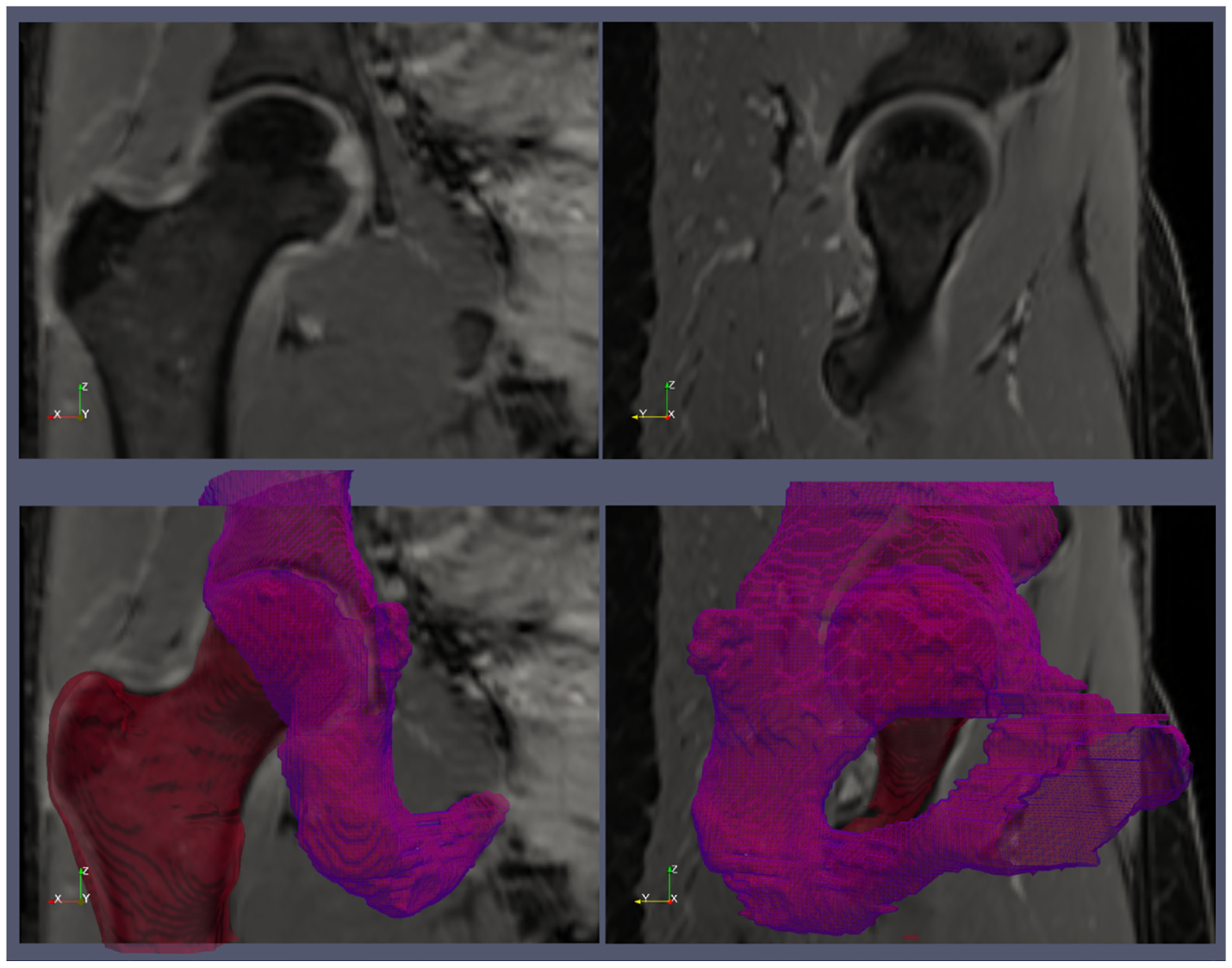
An example of the ground truth segmentation of the femur (red) and acetabulum (violet). The top row shows two water-only images from the Dixon MRI acquisition. The bottom row shows the 3D surfaces of the femur and acetabulum reconstructed from the regions of interests that were manually segmented on the MR images.

2.2. CNN for bone segmentation

We implemented a 3D CNN based on the U-Net architecture (Fig. 2) proposed by Cantarelli et al. [14], which was previously used for the automatic segmentation of the shoulder joint. The network is composed of four layers in the contracting/expanding paths with the number of features maps doubling in the contracting path and decreasing by a factor of two in the expanding one. In every layer, a convolution block is instantiated, each composed of a convolution operation and a ReLU. After the convolution block, the MaxPool operator is applied with a kernel size set of 2 × 2 × 1. The CNN was trained using the weighted cross-entropy (CE) loss function to overcome the imbalanced segmentation class problem [14]. This loss function can lead to a more balanced and effective training process by weighting the ROIs of interests, which comprise only a small portion of the image. In particular, the weights to prioritize the acetabulum and femur were calculated as follow.

Fig. 2.

Architecture of the 3D CNNs used in this work. The network was originally described in Ref. [14]. Blue rectangles represent feature maps with the size and the number of feature maps indicated on top of the bins. Different operations in the network are depicted by color-coded arrows.

The total number of pixels belonging to each ROI (acetabulum, femur, and background) was counted across all available training data. The pixel count for each ROI was then divided by the total number of pixels in all images. This resulted in a weight of 18.6 for the acetabulum, 15.83 for the femur, and 0.36 for the background. The weighted CE loss function was implemented as:

$$\mathit{\text{loss}}=\sum _i^L{w}_i*y_i*\text{log}\left(p_i\right)$$

where i iterates over all the L = 3 w_i ROIs (1 for acetabulum, 2 for femur, 0 for background), y_i is the weight assigned to i-th ROI is the ground truth value (0 or 1) for the i-th ROI at a specific pixel, and p_i is the predicted probability of the pixel belonging to the i-th ROI.

The optimization of this loss was conducted using an extension to stochastic gradient descent (ADAM) with a learning rate of 1e-4, a maximum number of iterations of 320, and an early stopping condition of 1e⁻⁸, as described in Ref. [14]. For all cases, the hip MR images and ROIs were re-sampled to the working resolution of the network in Ref. [14]. The final matrix size of the images and ROIs was 320 × 320 × 32 voxels.

2.3. Data augmentation

To increase the sample size, DA was applied by generating rototranslated couples of images and ROIs that were sampled at different resolutions. In particular, the 66 labeled and segmented femur and acetabulum ROIs were augmented by a factor of 60, which brought the total number of hip datasets from 66 to 3960.

Each augmentation involved extracting three Euler angles and three translation values, which were then used to create a roto-translation matrix as described in Refs. [25,26]. This rotation matrix was applied to both the image and the label, effectively transforming them according to the specified parameters.

In particular, the augmented datasets were obtained by creating randomly uniform 3D roto-translations between −5 and 5° in the first two Euler’s angles (left-right and anterior-posterior) and between −15 and 15° in the third Euler’s angle (inferior-superior), with random translations ranging between 5 and −5 mm applied to the full resolution images and ROIs. To maintain the anatomical shape of the hips as realistic as possible, no scaling was applied to the datasets [21].

To preserve the integrity of the labels, we used different interpolation methods for the image and label data. The image data was resampled using a b-spline interpolator, which produces smoother and continuous results. For the label data, we employed a nearest-neighbor approach to maintain the discrete label values without introducing any interpolation artifacts.

Of the 3960 available hips, 1560 augmented datasets, created from 13 patients, were randomly selected as the hold-out testing datasets for model evaluation. The remaining 2400 augmented datasets were used for model training. This split ensured that the testing dataset was representative of the training dataset and that the model was not overfitting the training data. The testing dataset was used to evaluate the performance of the trained model on unseen data. We ensured that the testing set was truly independent of the training set by avoiding augmented data from the same patient in both the training and the testing set.

2.4. Transfer learning

In addition to training the above-described CNN directly on the hip datasets, we evaluated whether we could improve performance by using TL from the model previously trained with the same CNN for the segmentation of the shoulder joint [14]. We were able to use the pre-trained CNN in a straightforward manner because the number of regions to be identified was identical in the two tasks (humerus and glenoid for the shoulder vs. femur and acetabulum for the hip). In addition, the shoulder MRI data used for training the model in Ref. [14] were acquired with the same pulse sequence and similar parameters. Specifically, they also used an axial dual-echo T1-weighted 3D fast low-angle shot (FLASH) sequence with Dixon fat-water separation, with TR = 10 ms, TEs = 2.4 ms, and 3.7 ms, field of view = 200 mm, acquisition matrix = 192 × 192, and slice thickness = 1 mm.

2.5. Model training comparison

To evaluate the effect of TL and DA on the final prediction accuracy of the models, we separately trained the network four times, using different training approaches:

• NTLNDA: No transfer learning, no DA, using only the available 66 hip datasets.

• NTLYDA: No transfer learning, using the 3960 augmented datasets.

• YTLNDA: Using transfer learning, with only the available 66 hip datasets.

• YTLYDA: Using transfer learning, with the 3960 augmented datasets.

The initial weights of the two networks without TL were set randomly. For TL, we initialized the weights of our new model with the weights of the previous model obtained from its checkpoints. After training, the four models were compared against the ground truth segmentations using features extracted from the confusion matrix. Each metric was compared to the other groups using a non-parametric test (Friedman test), with a null hypothesis of no differences in performance with a p-value of 0.01. The calculations were performed using the MATLAB statistical toolbox (The MathWorks Inc., Natick, MA). The segmentation results for the four models were also compared using the surface distance map Root Means Squared Difference (RMSD) [14].

The RMSD provides an average measure of how well the segmentation surface (S) generated by the network matches the ground truth surface (G), extracted from the ground truth manual segmentation. This metric was implemented as described in Deniz et al. [15], using the shortest Euclidean distance of an arbitrary voxel v to surface S defined as d(v, S) = min_s S||v −s||²

$$D=\sqrt{\frac{1}{N_S+N_G}\left({\sum }_{x_s\in S}d\left(x_s,G\right)+{\sum }_{x_G\in G}d\left(x_G,S\right)\right)}$$

where x_s and x_g are two arbitrary voxel in S and G, N_s and N_g represent the number of voxels in the segmentation and ground truth surface, respectively.

Note that, for all the comparisons during the validation, the segmentations were first re-sampled to the resolution of the ground truth segmentations (1 mm isotropic) using a nearest-neighbor approach.

3. Results

NTLYDA performed better than the other models in most metrics (Table 1). It had the highest accuracy (98.5% and 99.1%), Dice coefficient (84.2% and 89.3%), F1 score (84.2% and 89.3%), Jaccard index (72.8% and 80.9%), sensitivity (94% and 97.2%) and recall (94% and 97.2%), for the acetabulum and femur, respectively. For the acetabulum, it also yielded the highest precision (78.5%), specificity (98.9%), and lowest false negative and false positive rates (21.5% and 1.1%). YTLYDA had the highest specificity (99.2%) and precision rate for the femur region (83.4%), as well as the best performance in terms of femur false negative and false positive rates, with 16% and 0.8%, respectively. YTLNDA had the worst performance in all metrics.

Table 1.

Comparison of Deep Learning Models for Acetabulum and Femur Segmentation on 3D MR Images (Bolded values indicates the best performing method for each metric).

Metrics	NTLNDA	YTLYDA	NTLYDA	YTLNDA
Acetabulum Accuracy	0.946 ± (0.023)	0.980 ± (0.007)	0.985 ± (0.005)	0.931 ± (0.018)
Acetabulum Dice	0.610 ± (0.082)	0.783 ± (0.064)	0.842 ± (0.026)	0.473 ± (0.062)
Acetabulum Recall	0.940 ± (0.019)	0.832 ± (0.051)	0.912 ± (0.026)	0.713 ± (0.045)
Acetabulum F1	0.610 ± (0.082)	0.783 ± (0.064)	0.842 ± (0.026)	0.473 ± (0.062)
Acetabulum Sensitivity	0.940 ± (0.019)	0.832 ± (0.051)	0.912 ± (0.026)	0.713 ± (0.045)
Acetabulum Specificity	0.947 ± (0.024)	0.987 ± (0.006)	0.989 ± (0.005)	0.941 ± (0.017)
Acetabulum False Negative Rate	0.543 ± (0.084)	0.254 ± (0.101)	0.215 ± (0.055)	0.643 ± (0.063)
Acetabulum Jaccard	0.444 ± (0.080)	0.647 ± (0.087)	0.728 ± (0.039)	0.312 ± (0.055)
Acetabulum False Positive Rate	0.053 ± (0.024)	0.013 ± (0.006)	0.011 ± (0.005)	0.059 ± (0.017)
Acetabulum Precision	0.457 ± (0.084)	0.746 ± (0.101)	0.785 ± (0.055)	0.357 ± (0.063)
Femur Accuracy	0.974 ± (0.018)	0.991 ± (0.003)	0.991 ± (0.004)	0.961 ± (0.013)
Femur Dice	0.759 ± (0.101)	0.884 ± (0.043)	0.893 ± (0.042)	0.649 ± (0.098)
Femur Recall	0.972 ± (0.004)	0.946 ± (0.050)	0.968 ± (0.006)	0.934 ± (0.028)
Femur F1	0.759 ± (0.101)	0.884 ± (0.043)	0.893 ± (0.042)	0.649 ± (0.098)
Femur Sensitivity	0.972 ± (0.004)	0.946 ± (0.050)	0.968 ± (0.006)	0.934 ± (0.028)
Femur Specificity	0.974 ± (0.019)	0.992 ± (0.003)	0.992 ± (0.004)	0.962 ± (0.013)
Femur False Negative Rate	0.368 ± (0.119)	0.166 ± (0.065)	0.169 ± (0.069)	0.496 ± (0.112)
Femur Jaccard	0.620 ± (0.115)	0.795 ± (0.068)	0.809 ± (0.065)	0.488 ± (0.109)
Femur False Positive Rate	0.026 ± (0.019)	0.008 ± (0.003)	0.008 ± (0.004)	0.038 ± (0.013)
Femur Precision	0.632 ± (0.119)	0.834 ± (0.065)	0.831 ± (0.069)	0.504 ± (0.112)

Furthermore, NTLYDA had the lowest metrics standard deviation for both the acetabulum and the femur, which indicates that it is the most consistent model in its performance. All the features of the confusion matrix had a Friedman test p-value lower than the threshold of 0.01, making the differences in NTLYDA’s performance compared to the other three models statistically significant.

Fig. 3 shows the results of the RMSD analysis. NTLNDA had an error of 2.9 ± (0.27) mm on the acetabulum and 3.3 ± (0.37) mm on the femur. The results of the model trained with DA (NTLYDA and YTLYDA) were not statistically different, with an RMSD on the acetabulum of 2.1 ± (0.37) mm and 2.2 ± (0.44) mm, respectively, and 2.5 ± (0.65) mm and 2.9 ± (0.75) mm on the femur. The worst performance was found for YTLNDA, with an RMSD of 3.1 ± (0.24) mm on the femur and 4.2 ± (0.40) mm on the acetabulum.

Fig. 3.

Root Mean Square Deviation (RMDS) of the four DL models for the two anatomical regions. The RMDS is a measure of the average error (in mm) between the predicted and ground truth segmentations.

The ROC curves in Fig. 4 show that the models that used data augmentation (NTLYDA and YTLYDA) performed better than the other models. All the average areas under the curve (AUC) were higher than 0.90, except for the model YTLNDA on the acetabulum (0.873 ± (0.033)). The maximum mean AUC was found for NTLYDA, which achieved 0.954 ± (0.0064) and 0.973 ± (0.0033) for the acetabulum and the femur, respectively.

Fig. 4.

The receiver operating characteristic (ROC) analysis of the four DL models for the two regions of interest: acetabulum (left) and femur (right). The performance of YTLNDA was statistically different (p < 0.05) from the others for both femur and acetabulum.

NTLYDA also had the minimum distance from the point (0,1) (maximum sensitivity and specificity) for both the acetabulum (0.075) and the femur (0.032). The model that was furthest from the optimal point for the acetabulum was YTLNDA with a distance of 0.264, and the model that was furthest from the optimal point for the femur was NTLNDA with a distance of 0.139.

4. Discussion

The results of this study suggest that DA could be more beneficial than TL when limited data is available to train a CNN for the automatic segmentation of the bony structures of the hip joint. In fact, the model that used only augmented data (NTLYDA) was the most consistent and achieved the highest performance, followed by the model that used both transfer learning and data augmentation (YTLYDA).

TL from the shoulder segmentation network without using DA (YTLNDA) yielded the worst performance. While TL initially appeared promising, fine-tuning a model pre-trained for shoulder segmentation ultimately failed to achieve optimal performance for hip joint segmentation. This is primarily due to significant anatomical differences in the source and target domains of knowledge (shoulder vs hip), as highlighted in Fig. 5. The deep acetabulum of the hip joint is considerably different from the shallower glenoid fossa of the shoulder. This stark topological distinction challenged the transfer learning approach, causing the network to struggle to adapt its learned features from the shoulder to the unique morphology of the acetabulum (Fig. 6). This difficulty is further evidenced by the high rate of false negatives (0.643) observed for the acetabulum in the YTLNDA model (Table 1), which we reported also in previous work [18].

Fig. 5.

A qualitative comparison of the accuracy of the four DL models. Each row shows the segmentation obtained with a different DL model co-registered with the ground-truth manual segmentation (red and purple meshes), for a representative hip dataset and for different views. The closer a pixel color is to gray, the better the automatic segmentation matches the ground-truth at that pixel.

Fig. 6.

3D models of the hip (top) and the shoulder joint (bottom). The bony structures of the joints are shown in different colors: acetabulum (purple) and femur (red) for the hip joint, glenoid (purple), and humerus (red) for the shoulder joint. The femur and the humerus are similar in shape and size, while the acetabulum is a deeper socket than the glenoid fossa. To compare the size of the two joints across the two images, we added in both images a white sphere of radius equal to 1 cm.

In contrast, DA proved to be a far more effective strategy for overcoming these anatomical disparities. By diversifying the training data with synthetic variations of the hip joint images, DA exposed the network to a much broader range of anatomical configurations. This enabled the network to learn and generalize significantly better to unseen data, particularly those featuring the unique characteristics of the acetabulum. This is reflected in the dramatically lower false negative rate (0.21) achieved by the best data augmentation model (NTLYDA) compared to YTLNDA (0.64), clearly demonstrating the superiority of this regularization method.

We hypothesize that the already substantial size and diversity of the training data achieved through DA rendered the addition of TL counterproductive. The excessive regularization introduced by combining both approaches may have caused the model to become overly sensitive to specific features of the data, hindering its ability to generalize to unseen examples, especially those featuring the challenging acetabulum region (e.g. see the acetabulum ROI of YTLYDA in Fig. 5). This could explain the lower performance of YTLYDA compared to YTLNDA.

The accuracy of the NTLYDA model was consistent with the results of the shoulder segmentation model that was used for TL [14], which reported a sensitivity of 94.9% for the humerus and 85.6% for the glenoid, compared to 91.2% for the acetabulum and 96.8% for the femur of the NTLYDA model. The Dice coefficient of NTLYDA was 0.89% for the femur and 0.84% for the acetabulum, while it was 0.95% for the humerus and 0.86% for the glenoid in Ref. [14].

A previous study for the automatic segmentation of the hip joint reported a higher Dice coefficient of 97% for the femur and 98% for the acetabulum [3]. Such study used a custom-reduced field of view (FOV) of the hip MR images to automatically segment only the area where the femur articulates with the acetabulum. This approach decreases the risk of false positive segmentations and was proven effective in segmenting the junction between the two structures for ROM analysis. In our case, we decided to maintain a broader coverage of the femur and acetabulum in the images, because this can improve the outcome if the segmented bones are used for radiomics analysis [28]. In fact, radiomic features are often derived from the spatial distribution of intensity values in an image and this distribution can vary significantly if the size of the ROI is reduced [33].

The reported RMSD is a measure of the average distance between the surface of the ground truth segmentations and the segmentations produced by the DL models. The models that were trained with DA had lower RMSD values for both the acetabulum and the femur with a decrease in error of over 25% compared to the model trained only with the available patients’ data (NTLNDA). For the femur, the average RMSD value was slightly higher than the acetabulum but both models were able to decrease the error by over 35% using DA. This decrease in error can be attributed to several factors. First, by artificially increasing the size of the training data, DA might have reduced overfitting, which is typical of DL models trained on a small set of data, allowing the model to effectively generalize to new data. Second, DA might have helped to improve the robustness of the model. In fact, the model trained with the augmented dataset was exposed to a wider variety of cases, which could have helped it to learn to identify and segment the anatomical structures for different rotations and translations of the hip joint.

Even if the use of DA and TL decreased the RMSD, its value remained slightly higher than the RMSD reported in Ref. [14] for the shoulder model, which was trained on data from 100 patients. This might depend on the fact that, in order to use the same network in Ref. [14] for TL, we needed to interpolate our hip MRI data to a resolution of 0.4 × 0.4 × 3.8 mm. This low resolution along the z-axis prevents capturing some of the anatomical details and could have impaired the ability of the model to accurately segment the bony structures of the hip joint. At the same time, the 3.8 mm resolution along the z-axis explains why the average RMSD is more than 2 mm for all cases. Another limitation of this study was that the architecture of the network was fixed to the one used in Ref. [14]. This was necessary in order to utilize the checkpoints of the network trained on the shoulder as the initialization weights for the hip network in the case of comparison of DA with TL.

Note that zero-shot and foundation models have been recently introduced for object detection and segmentation [34,35]. However, the performance of these methods is not consistent for different applications, as shown in a recent review article [36]. In particular, such work used 12 publicly available datasets covering different organs and including various image modalities. The observed performance variations across these datasets and tasks suggest that current general-purpose pre-trained models, such as Segment Anything, may not possess the necessary stability and accuracy to reliably achieve zero-shot segmentation on complex, multi-modal, and multi-target medical data [36]. In this work, we instead decided to implement a CNN U-net tailored to our specific segmentation task.

This study focused solely on segmenting the bony structures of the hip joint, so the generalizability of the results for the case of other anatomical structures remains to be determined. For example, the unique features and challenges specific to the hip joint, such as the deep socket of the acetabulum, may be the reason for the suboptimal performance of TL compared to DA. Therefore, further research is necessary to confirm that DA is a better approach than TL when only small training sets are available.

A final limitation of our study was the skewed gender distribution of our patient population (16 females vs. 4 males). However, note that there were no major gender-related differences in segmentation performance metrics on the test cohort of patients, which suggests that the developed models perform equally well for males and females.

5. Conclusions

In conclusion, this study investigated the effect of DA and TL on the accuracy of a CNN for the automatic segmentation of the bony structures of the hip joint from MR images, for cases when a limited number of datasets is available. We found that DA has a larger impact than TL on the network performance, likely because it reduces overfitting. TL still has a beneficial effect, but the associated performance depends on how similar the available data are compared to those used to train the original model. The proposed network for hip bone segmentation could be combined with radiomic analysis [28] to make the diagnosis of FAIS completely automatic. In the future, we plan to explore the relationship between the complexity of the network and the accuracy of the estimation by using different network architectures and DA.

References

- [1].Griffin DR, Dickenson EJ, O’Donnell J, Agricola R, Awan T, Beck M, Clohisy JC, Dijkstra HP, Falvey E, Gimpel M, Hinman RS, Hölmich P, Kassarjian A, Martin HD, Martin R, Mather RC, Philippon MJ, Reiman MP, Takla A, Bennell KL. The Warwick Agreement on femoroacetabular impingement syndrome (FAI syndrome): an international consensus statement. Br J Sports Med 2016;50(19):1169–76. 10.1136/bjsports-2016-096743. [DOI] [PubMed] [Google Scholar]
- [2].Naili JE, Stålman A, Valentin A, Skorpil M, Weidenhielm L. Hip joint range of motion is restricted by pain rather than mechanical impingement in individuals with femoroacetabular impingement syndrome. Arch Orthop Trauma Surg 2021. 10.1007/s00402-021-04185-4. [DOI] [PMC free article] [PubMed] [Google Scholar]
- [3].Zeng G, Degonda C, Boschung A, Schmaranzer F, Gerber N, Siebenrock KA, Steppacher SD, Tannast M, Lerch TD. Three-dimensional magnetic resonance imaging bone models of the hip joint using deep learning: dynamic simulation of hip impingement for diagnosis of intra- and extra-articular hip impingement. Orthop J Sports Med 2021;9(12). 10.1177/23259671211046916. [DOI] [PMC free article] [PubMed] [Google Scholar]
- [4].Kubiak-Langer M, Tannast M, Murphy SB, Siebenrock KA, Langlotz F. Range of motion in anterior femoroacetabular impingement. Clin Orthop Relat Res 2007; 458:117–24. 10.1097/BLO.0b013e318031c595. [DOI] [PubMed] [Google Scholar]
- [5].Whiteside D, Deneweth JM, Bedi A, Zernicke RF, Goulet GC. Femoroacetabular impingement in elite ice hockey goaltenders: etiological implications of on-ice hip mechanics. Am J Sports Med 2015;43(7):1689–97. 10.1177/0363546515578251. [DOI] [PubMed] [Google Scholar]
- [6].Beaulé PE, Zaragoza E, Motamedi K, Copelan N, Dorey FJ. Three-dimensional computed tomography of the hip in the assessment of femoroacetabular impingement. J Orthop Res 2005;23(6):1286–92. 10.1016/j.orthres.2005.03.011. [DOI] [PubMed] [Google Scholar]
- [7].Frank JM, Harris JD, Erickson BJ, Slikker W, Bush-Joseph CA, Salata MJ, Nho SJ. Prevalence of femoroacetabular impingement imaging findings in asymptomatic volunteers: a systematic review. Arthrosc J Arthrosc Relat Surg 2015;31(6): 1199–204. 10.1016/j.arthro.2014.11.042. [DOI] [PubMed] [Google Scholar]
- [8].Tannast M, Siebenrock KA, Anderson SE. Femoroacetabular impingement: radiographic diagnosis–what the radiologist should know. AJR. Am J Roentgenol 2007;188(6):1540–52. 10.2214/AJR.06.0921. [DOI] [PubMed] [Google Scholar]
- [9].Bedi A, Thompson M, Uliana C, Magennis E, Kelly BT. Assessment of range of motion and contact zones with commonly performed physical exam manoeuvers for femoroacetabular impingement (FAI): what do these tests mean? HIP Int 2013; 23(SUPPL. 9). 10.5301/hipint.5000060. [DOI] [PubMed] [Google Scholar]
- [10].Samim M, Eftekhary N, Vigdorchik JM, Elbuluk A, Davidovitch R, Youm T, Gyftopoulos S. 3D-MRI versus 3D-CT in the evaluation of osseous anatomy in femoroacetabular impingement using Dixon 3D FLASH sequence. Skeletal Radiol 2019;48(3):429–36. 10.1007/s00256-018-3049-7. [DOI] [PubMed] [Google Scholar]
- [11].Lerch TD, Degonda C, Schmaranzer F, Todorski I, Cullmann-Bastian J, Zheng G, Siebenrock KA, Tannast M. Patient-specific 3-D magnetic resonance imaging–based dynamic simulation of hip impingement and range of motion can replace 3-D computed tomography–based simulation for patients with femoroacetabular impingement: implications for planning open hip preservation surgery and hip arthroscopy. Am J Sports Med 2019;47(12):2966–77. 10.1177/0363546519869681. [DOI] [PubMed] [Google Scholar]
- [12].Wylie JD, Jenkins PA, Beckmann JT, Peters CL, Aoki SK, Maak TG. Computed tomography scans in patients with young adult hip pain carry a lifetime risk of malignancy. Arthrosc J Arthrosc Relat Surg 2018;34(1):155–163.e3. 10.1016/j.arthro.2017.08.235. [DOI] [PubMed] [Google Scholar]
- [13].Gyftopoulos S, Yemin A, Mulholland T, Bloom M, Storey P, Geppert C, Recht MP. 3DMR osseous reconstructions of the shoulder using a gradient-echo based two-point Dixon reconstruction: a feasibility study. Skeletal Radiol 2013;42(3):347–52. 10.1007/s00256-012-1489-z. [DOI] [PubMed] [Google Scholar]
- [14].Cantarelli Rodrigues T, Deniz CM, Alaia EF, Gorelik N, Babb JS, Dublin J, Gyftopoulos S. Three-dimensional MRI bone models of the glenohumeral joint using deep learning: evaluation of normal anatomy and glenoid bone loss. Radiology: Artif Intell 2020;2(5):e190116. 10.1148/ryai.2020190116. [DOI] [PMC free article] [PubMed] [Google Scholar]
- [15].Deniz CM, Xiang S, Hallyburton RS, Welbeck A, Babb JS, Honig S, Cho K, Chang G. Segmentation of the proximal femur from MR images using deep convolutional neural networks. Sci Rep 2018;8(1). 10.1038/s41598-018-34817-6. [DOI] [PMC free article] [PubMed] [Google Scholar]
- [16].Tajbakhsh N, Jeyaseelan L, Li Q, Chiang JN, Wu Z, Ding X. Embracing imperfect datasets: a review of deep learning solutions for medical image segmentation. Med Image Anal 2020;63:101693. 10.1016/J.MEDIA.2020.101693. [DOI] [PubMed] [Google Scholar]
- [17].Buja Werner Stuetzle Shen Yi. Cross-validation: a powerful tool for model evaluation by Andreas Buja, Werner Stuetzle, and yi shen. Am Statistician Aug., 2007;61(No. 3):198–209. [Google Scholar]
- [18].Montin E, Deniz CM, Rodrigues TC, Gyftopoulos S, Kijowski R, Lattanzi R. Automatic segmentation of the hip bony structures on 3D Dixon MRI datasets using transfer learning from a neural network developed for the shoulder. In: 30th Scientific Meeting of the International Society for Magnetic Resonance in Medicine (ISMRM) London (UK), 07–12 May 2022; 2022. p. 1412. [Google Scholar]
- [19].Zhuang F, Qi Z, Duan K, Xi D, Zhu Y, Zhu H, Xiong H, He Q. A comprehensive survey on transfer learning. In: Proceedings of the IEEE, vol. 109. Institute of Electrical and Electronics Engineers Inc; 2021. p. 43–76. 10.1109/JPROC.2020.3004555. Issue 1. [DOI] [Google Scholar]
- [20].Kim HE, Cosa-Linan A, Santhanam N, et al. Transfer learning for medical image classification: a literature review. BMC Med Imag 2022;22:69. 10.1186/s12880-022-00793-7. [DOI] [PMC free article] [PubMed] [Google Scholar]
- [21].Valverde JM, Imani V, Abdollahzadeh A, de Feo R, Prakash M, Ciszek R, Tohka J. Transfer learning in magnetic resonance brain imaging: a systematic review. J Imaging 2021;7(Issue 4). 10.3390/jimaging7040066. MDPI. [DOI] [PMC free article] [PubMed] [Google Scholar]
- [22].Ham S, Kim M, Lee S, Wang C, Ko B, Kim N. Improvement of semantic segmentation through transfer learning of multi-class regions with convolutional neural networks on supine and prone breast MRI images. Sci Rep 2023;13(1):1–8. 10.1038/s41598-023-33900-x. [DOI] [PMC free article] [PubMed] [Google Scholar]
- [23].Mumuni A, Mumuni F. Data augmentation: a comprehensive survey of modern approaches. Array 2022;16:100258. 10.1016/j.array.2022.100258. [DOI] [Google Scholar]
- [24].Shorten C, Khoshgoftaar TM. A survey on image data augmentation for deep learning. J Big Data 2019;6:60. 10.1186/s40537-019-0197-0. [DOI] [PMC free article] [PubMed] [Google Scholar]
- [25].McCormick M, Liu X, Jomier J, Marion C, Ibanez L. ITK: enabling reproducible research and open science. Front Neuroinf 2014;8(13). 10.3389/fninf.2014.00013. Published 2014 Feb 20. [DOI] [PMC free article] [PubMed] [Google Scholar]
- [26].Yoo TS, Ackerman MJ, Lorensen WE, Schroeder W, Chalana V, Aylward S, Metaxas D, Whitaker R. Engineering and algorithm design for an image processing API: a technical report on ITK – the insight toolkit. In: Westwood J, editor. Proc. Of medicine meets virtual reality. IOS Press Amsterdam; 2002. p. 586–92. [PubMed] [Google Scholar]
- [27].Schmid J, Assassi L, Chênes C. A novel image augmentation based on statistical shape and intensity models: application to the segmentation of hip bones from CT images. Eur Radiol Exp 2023;7:39. 10.1186/s41747-023-00357-6. [DOI] [PMC free article] [PubMed] [Google Scholar]
- [28].Montin E, Kijowski R, Youm T, Lattanzi R. A radiomics approach to the diagnosis of femoroacetabular impingement. Front Radiol 2023;3. 10.3389/fradi.2023.1151258. [DOI] [PMC free article] [PubMed] [Google Scholar]
- [29].Zhang C, Bengio S, Hardt M, Recht B, Vinyals O. Understanding deep learning (still) requires rethinking generalization. Commun ACM 2021;64(3):107–15. 10.1145/3446776. [DOI] [Google Scholar]
- [30].Shorten C, Khoshgoftaar TM. A survey on image data augmentation for deep learning. J Big Data 2019;6(1). 10.1186/s40537-019-0197-0. [DOI] [PMC free article] [PubMed] [Google Scholar]
- [31].Chen C, Qin C, Ouyang C, Li Z, Wang S, Qiu H, Chen L, Tarroni G, Bai W, Rueckert D. Enhancing MR image segmentation with realistic adversarial data augmentation. Med Image Anal 2022;82:102597. 10.1016/j.media.2022.102597. [DOI] [PubMed] [Google Scholar]
- [32].Yushkevich PA, Piven J, Cody Hazlett H, Gimpel Smith R, Ho S, Gee JC, Gerig G. User-guided 3D active contour segmentation of anatomical structures: significantly improved efficiency and reliability. Neuroimage 2006;31(3):1116–28. [DOI] [PubMed] [Google Scholar]
- [33].Bibault JE, Xing L, Giraud P, el Ayachy R, Giraud N, Decazes P, Burgun A. Radiomics: a primer for the radiation oncologist. Cancer Radiother 2020;24(Issue 5):403–10. 10.1016/j.canrad.2020.01.011. Elsevier Masson SAS. [DOI] [PubMed] [Google Scholar]
- [34].Passa R, Nurmaini S, Rini D. YOLOv8 based on data augmentation for MRI brain tumor detection. Sci J Inform 2023;10(3):363–70. 10.15294/sji.v10i3.45361. [DOI] [Google Scholar]
- [35].Shi P, Qiu J, Abaxi SMD, Wei H, Lo FP, Yuan W. Generalist vision foundation models for medical imaging: a case study of segment anything model on zero-shot medical segmentation. Diagnostics 2023;13(11). 10.3390/diagnostics13111947. 1947. Published 2023 Jun 2. [DOI] [PMC free article] [PubMed] [Google Scholar]
- [36].Zhang Y, Jiao R. Towards segment anything model (SAM) for medical image segmentation. A Survey; 2023.