Thermodynamic Properties of cis-1,1,1,4,4,4-Hexafluorobutene [R‑1336mzz(Z)]: Vapor Pressure, (p, ρ, T) Behavior, and Speed of Sound Measurements and Equation of State

Abstract

We present experimental measurements of the density, speed of sound, vapor pressure, and dew-point pressure of cis-1,1,1,4,4,4-hexafluorobutene, which is also known as R-1336mzz(Z). Vapor pressures were measured at temperatures from 330 to 440 K; the dew-point pressure was measured at T = 293.15 K. Densities were measured in the liquid and supercritical regions over the temperature range of 230 to 460 K, with pressures up to 36 MPa. Vapor-phase sound speeds were measured at temperatures between 280 and 480 K, with pressures from 0.021 to 2.2 MPa. Densities and dew points were measured in a two-sinker densimeter with a magnetic suspension coupling. Vapor pressures were measured with a static technique in the densimeter. Sound speed data were measured with a spherical acoustic resonator. An equation of state written in terms of the Helmholtz energy was developed based on these data together with additional data from the literature; it represents the present experimental data with relative average absolute deviations (AAD) of 0.0081% for densities, 0.027% for vapor pressure, and 0.017% for vapor-phase speed of sound. Literature data for liquid-phase speed of sound have an AAD of 0.023%, and for saturated liquid density data, the AAD is 0.049%.

Graphical Abstract

1. INTRODUCTION

The compound cis-1,1,1,4,4,4-hexafluorobutene (CAS 692–49-9), also known as R-1336mzz(Z), with chemical formula C₄H₂F₆ and a molar mass of 164.056 g·mol⁻¹, is an unsaturated hydrofluorocarbon, which has been developed as a working fluid for organic Rankine (ORC) power cycles, as a refrigerant for use in chillers, and as a foam-blowing agent. This compound has been approved by the U.S. Environmental Protection Agency as a blowing agent in rigid and flexible polyurethane foams, as a refrigerant in chillers, and as a cleaning solvent.¹ R-1336mzz(Z) forms an azeotrope with trans-1,2-dichloroethene (R-1330(E)); this blend is known as R-514A in ANSI/ASHRAE Standard 34.²

R-1336mzz(Z) has a relatively short atmospheric lifetime of 22 days due to the presence of a carbon−carbon double bond in the molecule.³ This is much lower than the atmospheric lifetime of other refrigerants used in similar applications, e.g., 7.7 years in the case of HFC-245fa.³ It has a global warming potential of 2 relative to carbon dioxide at an integration time horizon of 100 years (GWP₁₀₀),³ as compared to a GWP₁₀₀ of 858 for HFC-245fa.³ It has zero ozone depletion potential (ODP). This compound is of low toxicity, and it is not flammable as indicated by its safety classification of “A1” in ANSI/ASHRAE Standard 34.²

Only very limited experimental data for the thermodynamic properties of this compound are available in the literature, and these are discussed in section 4.2. Increasing the available high-quality experimental data as well as providing a reliable equation of state will enable a robust evaluation of the commercial utility of R-1336mzz(Z).

In the present work, (p, ρ, T) data are reported at temperatures ranging from 230 to 460 K, with pressures up to 36 MPa. Sound speed data were measured with temperatures between 280 and 480 K, with pressures from 0.021 to 2.2 MPa. Vapor pressures were measured at temperatures from 330 to 440 K; the dew-point pressure was measured at T = 293.15 K.

An equation of state explicit in the Helmholtz energy was fitted to the experimental data reported in this work together with selected literature data. Experimental data, including data reported by other authors, are compared with the equation of state. The equation of state is of a form compatible with the NIST REFPROP database.⁴

2. EXPERIMENTAL SECTION

2.1. Experimental Sample.

The sample of cis-1,1,1,4,4,4-hexafluorobutene was supplied in a 1000 cm³ steel gas cylinder and was of high purity, as detailed in Table 1. The sample, as received, was packaged under nitrogen and was degassed before the present measurements were undertaken. The sample was transferred to a 1000 cm³ stainless steel gas cylinder, and 11 cycles of freezing in liquid nitrogen, evacuating the vapor space, and thawing were carried out. The pressure in the vapor space over the frozen material was <1·10⁻⁴ Pa on the final degassing cycle.

Table 1.

Sample Information

chemical name	sourcec	initial purity/mole fraction	purification method	final purity/mole fraction	analysis method
R-1336mzz(Z)a	Chemours	∼0.9999	degassing	∼0.9999	GC/QToF-MSb
argon	Matheson	0.999999	none		supplier’s assay

^acis-1,1,1,4,4,4-Hexafluorobutene.

^bGas chromatography/quadrupole time-of-flight mass spectroscopy.

^cCommercial materials are identified only to adequately specify the experiment.

In no case does such identification imply a recommendation or endorsement by the National Institute of Standards and Technology nor does it imply that the products identified are necessarily the best available for the purpose.

A purity analysis by gas-chromatography/quadrupole time-of-flight mass spectroscopy (GC/QToF-MS) was carried out at NIST. A 30 m long capillary column coated with 5% phenyl/95% dimethylpolysiloxane was used for the separation. Only a single peak was detected with a “normal” injection of sample volume; only by overloading the detector was a second minor peak detected. The minor peak could not be identified, but the spectra was consistent with a fluorinated compound. Although a quantitative statement of purity is not possible, we conclude that the sample was “very pure” (∼ 99.99% molar purity). An analysis of the sample removed from the two-sinker densimeter following the density measurements was also carried out; no significant differences were observed.

2.2. Apparatus Descriptions.

2.2.1. Two-Sinker Densimeter with Magnetic Suspension Coupling.

The present measurements utilized a two-sinker densimeter with a magnetic suspension coupling. This type of instrument applies the Archimedes (buoyancy) principle to provide an absolute determination of the density. This general type of instrument is described by Wagner and Kleinrahm,⁵ and our instrument is described in detail by McLinden and Lösch-Will.⁶ Briefly, two sinkers of nearly the same mass (∼60 g) and same surface area (∼41.5 cm²), but very different volumes, were each weighed with a high-precision balance while they were immersed in the sample of unknown density. The basic form of the working equation for this type of instrument gives the fluid density ρ as

$$\rho =\frac{\left(m_1-m_2\right)-\left(W_1-W_2\right)}{\left(V_1-V_2\right)}$$ (1)

where m and V are the mass and volume of the sinkers, W is the balance reading when weighing a sinker, and the subscripts refer to the two sinkers. One sinker was made of tantalum (m = 60.094 633 g, V = 3.60 872 cm³) and the other of titanium (m = 60.075 386 g, V = 13.315 284 cm³). A magnetic suspension coupling transmitted the gravity and buoyancy forces on the sinkers to the balance, thus isolating the fluid sample from the balance. With the two-sinker method, the systematic errors from the weighing and many other sources approximately cancel.

In addition to the sinkers, two calibration masses (designated m_cal and m_tare) were also weighed by placing them directly on the balance pan. This provided a calibration of the balance and also the information needed to correct for magnetic effects, as described by McLinden et al.⁷ The four weighings (two sinkers and two calibration masses) yielded a set of four equations that were solved to yield a balance calibration factor α and a parameter ϕ characterizing the efficiency of the magnetic suspension coupling. With these additional terms, the fluid density is

$${\rho }_{\text{fluid}}=\left\{\left[\left(m_1-m_2\right)-\frac{W_1-W_2}{\alpha \varphi }\right]/\left(V_1-V_2\right)\right\}-{\rho }_0$$ (2)

where ρ₀ is the indicated density when the sinkers are weighed in vacuum. In other words, ρ₀ is an “apparatus zero”. The density given by eq 2 compensates for the magnetic effects of both the apparatus and the fluid being measured. The difference of the value of ϕ from 1 indicates the magnitude of the force transmission error.⁷ For the present measurements, ϕ varied from 1.000 006 in vacuum to 0.999 953 for the liquid at a density of 1244 kg·m⁻³.

The densimeter was thermostated by means of a multilayer, vacuum-insulated thermostat. A copper shield with heaters at the top and side surrounded the measuring cell. An additional isothermal shield with heaters at the top and sides and a fluid cooling channel at the top surrounded the “inner shield”; it was maintained at a temperature approximately 1 K below the measuring-cell temperature. A chiller that circulated ethanol was used at temperatures below room temperature.

The temperature was measured with a 25 Ω standard platinum resistance thermometer (SPRT) and an AC resistance bridge referenced to a thermostated standard resistor. The temperature inside the measuring cell was constant within 2 mK. Pressures were measured with one of three vibrating-quartz-crystal-type pressure transducers having full-scale pressure ranges of 2.8, 13.8, or 69 MPa. The transducers and pressure manifold were thermostated at T = 313.15 K to minimize the effects of variations in laboratory temperature.

2.2.2. Spherical Acoustic Resonator.

The spherical acoustic resonator is a widely used method for the experimental determination of the speed of sound in gases. Detailed descriptions of the design and theory of spherical acoustic resonators can be found in Moldover et al.^8,9 and Trusler.¹⁰ The apparatus used in this work is described by Perkins and McLinden.¹¹ Only a brief summary is given here.

The resonator consisted of two flanged, stainless steel hemispheres, which were bolted together to form a spherical sample volume with an internal diameter of 80 mm. It had a working temperature range of 265 to 500 K, with pressures up to 40 MPa (however, smaller ranges of both T and p were measured here). Sound transducer ports were located in the top hemisphere, with an angular separation of 90° to reduce the interference between the (0, 2) and the (3, 1) modes. A sinusoidal excitation voltage was generated by a synthesized function generator.

The working equation of a spherical resonator relates the sound speed w to the sphere radius a and measured resonance frequency f_ln:

$$f_{ln}+i\cdot g_{ln}={\nu }_{ln}\left(\frac{w}{2\pi a}\right)+\sum _j\left(\mathrm{\Delta }{f}_j+i\cdot g\right)$$ (3)

where g_ln is the half-power bandwidth, the subscripts l and n refer to the resonance mode, and the eigenvalues ν_ln are the “turning points” (zeros of the first derivatives) of the spherical Bessel functions of order l. The summation accounts for corrections to the ideal model; the main contributions to this term come from the effect of the thermal boundary layer, the coupling between gas and shell motion, the fluid dissipation, and the presence of the filling tubes and the drive and detector transducers. These corrections totaled 0.12 Hz or less, corresponding to 0.0021% or less in the speed of sound. The transport properties needed to calculate these corrections were taken from Huber.¹² Full details on the boundary layer corrections are provided in Supporting Information. Small variations from a perfect sphere have a small effect on the measurements since only radially symmetric modes were measured.⁹

The radius of the sphere as a function of temperature and pressure was determined by measurements on high-purity argon, as described by Perkins and McLinden.¹¹ We used that calibration of the sphere radius for the present measurements. We did, however, confirm the calibration in the course of the current work by further measurements on high-purity argon (detailed in Table 1) over a temperature range of 275 to 500 K, with pressures near 0.5 MPa.

The resonator was thermostated by means of a multilayer, vacuum-insulated thermostat similar to that of the densimeter. A chiller that circulated water was used to operate the resonator at temperatures below room temperature. The temperature of the resonator cell was measured with a 25 Ω SPRT inserted into a thermowell in the flange of the sphere. The temperature inside the sphere was constant within 5 mK.

The pressure of the fluid was measured with a vibrating-quartz-crystal-type transducer with a full scale pressure range of 2.8 MPa. The fluid sample was loaded into the system by means of a manual, high-pressure, piston-type pump. Frequencies for the present measurements were between 1778 and 8883 Hz for the (0, 2) through (0, 5) radial modes.

2.3. Measurement Procedures.

2.3.1. Vapor Pressure.

Vapor pressures were measured in the two-sinker densimeter with a static technique. Approximately 50 cm³ of liquid sample (enough to fill the measuring cell 40% full) was loaded into the measuring cell, and measurements were made over a range of temperature, starting at 330 K and increasing to 440 K. At temperatures of 410 K and lower the “low-range” pressure transducer (p_max = 2.8 MPa) was used; above this temperature, it was valved out and the “medium-range” transducer (p_max = 13.8 MPa) was used. Both transducers were recorded at T = 400 and 410 K. A single vapor-pressure determination consisted of multiple measurements of the temperature and pressure after equilibrium was reached. (The sinker weighings were disabled.) Since the filling line was at the bottom of the cell, it was at least partially filled with liquid, and a hydrostatic head correction must be applied to the pressure reading. At cell temperatures above about 320 K, the pressure in the cell was above the dew point at the pressure transducer, and the pressure/filling line was completely filled with liquid; thus, the hydrostatic head correction could be applied with low uncertainty. At lower cell temperatures, the pressure line would be only partially filled with liquid, and the exact location of the liquid/vapor interface was not known. Because of this uncertainty and the relatively high normal boiling point temperature of 306.5 K for R-1336mzz(Z), measurements were not attempted below T = 330 K. After completing the measurement sequence at temperatures up to 440 K, the cell was cooled and replicate measurements (on the same sample) were made over the temperature range 330 to 360 K to check for possible sample degradation.

2.3.2. Dew-Point Pressure.

Because of the increasing uncertainties in the vapor-pressure measurements at low temperatures, the dew point was measured at T = 293.15 K to provide a low-pressure saturation data point. For a pure fluid, the dew-point and bubble-point pressures at a given temperature are the same; the dew point approaches saturation from the vapor side. A dew-point measurement comprised a (p, ρ, T) isotherm starting at a low pressure (20 to 50 kPa); the pressure was increased in steps of 1 to 10 kPa by cycling two pneumatic valves piped in series to introduce additional gaseous sample. As the pressure reached the dew point, the value of the coupling parameter ϕ (discussed in section 2.2.1) increased dramatically because of adsorption and condensation onto the sinkers; the intersection of lines fitted to the single-phase and two-phase data yielded the dew point. This effect and its exploitation for the measurement of dew points is discussed by McLinden and Richter.¹³ With this technique, the filling/pressure line was completely vapor filled up to the dew-point pressure, minimizing uncertainties in the hydrostatic head correction. An additional advantage is that a dew-point measurement is much less sensitive to the presence of a noncondensable impurity (such as air) compared to a bubble-point measurement. Three replicate isotherms, each starting with fresh sample, were carried out.

2.3.3. (p, ρ, T) Data.

A combination of measurements along isochores and along isotherms was carried out. The evacuated measuring cell was cooled and then filled with liquid directly from the sample bottle (which was heated); higher pressures were obtained by closing the valve to the sample bottle and then increasing the cell temperature in steps along a pseudoisochore. Once a new set point temperature and pressure was reached, an additional equilibration time of 40 min was allowed; five or more replicate density determinations were then carried out. When the maximum desired pressure along a pseudoisochore was reached, a portion of the sample was vented into a waste bottle to decrease the pressure; measurements were made in this manner along an isotherm to a minimum pressure of approximately 1 MPa. Measurements then resumed at increasing temperatures along the next, lower-density pseudoisochore. This procedure did not require any pump and thus avoided any chance for sample contamination that a pump or compressor might introduce; it also minimized the number of manual sample-handling steps.

Two primary fillings of the densimeter were used. The first filling covered the liquid phase over a temperature range of 230 to 430 K. Temperatures for the second filling ranged from 280 to 460 K and extended into the supercritical region. For the third filling, the sample was “recycled” from the waste bottle, and the densities were measured at T = 280 K; this isotherm served to check the reproducibility of the density after taking the sample to high temperature and high pressure.

Between each of the fillings, and also before and after all of the R-1336mzz(Z) testing, the densimeter cell was evacuated for a minimum of 36 h. This was done to clear the previously measured sample and to check the zero of the pressure transducers and the ρ₀ of the apparatus (eq 2). The ρ₀ varied by less than 0.0016 kg·m⁻³.

2.3.4. Speed of Sound, Spherical Resonator.

Sound speed measurements were carried out in the gas phase along 11 isotherms between 280 and 480 K, with pressures between 0.021 and 2.2 MPa. For each isotherm, fresh sample was loaded into the spherical resonator by means of a manual piston-type pump to a pressure equal to approximately 80% of the vapor pressure at that temperature. The sample was introduced as liquid, and it vaporized as it entered the sphere. The isotherm was measured at several pressure steps down to the minimum pressure. The resonator was evacuated between isotherms to ensure that a completely fresh sample was filled in for the following isotherm. The zero of the pressure transducer was also checked during this evacuation, and no significant changes were observed. In addition to the isotherms, two isochores spanning wide temperature ranges were also measured.

After the sample was loaded, the system was allowed to come to the set-point temperature and pressure; an additional 60 min was allowed for complete equilibration before starting the measurements. An initial frequency scan was carried out to locate the resonance peaks; this procedure is detailed by Perkins and McLinden.¹¹ The four radial modes from (0, 2) through (0, 5) were then scanned. Each scan consisted of 25 measurements spanning a frequency range of approximately 1.5 times the half-power bandwidth; a settling time of 5 s was allowed between frequencies. Each mode was scanned twice, with increasing and decreasing frequencies; this sequence required 27 min. The complete sequence was repeated three or more times to yield a total of at least 24 resonance scans at each (T, p) state point.

The raw data from the frequency scans, as well as the readings from the thermometers, the pressure transducer, etc., were stored to a file for off-line analysis. The (0, 3) and (0, 4) modes yielded calculated speeds of sound that were very consistent (average difference of 0.0041%). The speed of sound data calculated from the (0, 2) mode, on the other hand, were often systematically 0.46% higher than the (0, 3) mode for temperatures of 360 K and above; this was due to the peak-finding algorithm measuring the adjacent (3, 1) mode. The (0, 2) mode showed smaller (order of 0.02%) systematic deviations at other temperatures, and also, the signal was much weaker compared to the (0, 3) and (0, 4) modes. The sound speeds from the (0, 5) mode were systematically lower than the (0, 3) and (0, 4) modes by an average of 0.027%; the resonance for this mode was also much weaker, as indicated by a half-power bandwidth that was 2.5 to 4.0 times larger than the (0, 3) and (0, 4) modes. The differences seen with the (0, 5) mode might have been due to vibrational relaxation effects, but these were not investigated further. For these reasons, only the (0, 3) and (0, 4) modes were used in the final data analysis. For selected state points at temperatures of 460 K and higher, multiple replicate scans were carried out over the course of many hours to check for possible sample degradation at high temperatures.

2.3.5. Speed of Sound, Pulse−Echo Instrument.

Additional speed of sound measurements in the liquid phase were carried out at NIST in a pulse-echo instrument. These cover a temperature range of 230 to 420 K, with pressures up to 46 MPa. These measurements at 183 (T, p) state points along 12 isochores are reported elsewhere.¹⁴

3. RESULTS

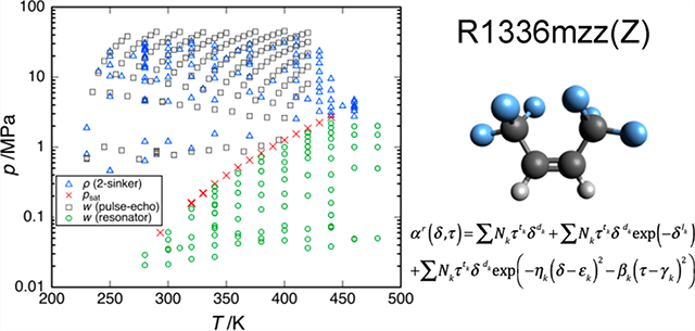
Figure 1 depicts the state points for the vapor pressures, dew-point pressures, densities, and speeds of sound measured in this work. These data are reported in Tables 2–5 and are described in the following sections. The relative combined, expanded uncertainties in the measured data (as discussed in section 3.4) are also given. The tables report only an average of the replicate points; data for all the replicates are available in Supporting Information. Comparisons of the experimental values with the values calculated from the new equation of state are given in section 4.2.

Figure 1.

Data measured for R-1336mzz(Z) in the present work: ×, vapor pressure and dew-point pressure; △, (p, ρ, T); ○, vapor-phase speed of sound in a spherical resonator (the solid lines connect points measured along two isochores); and □, liquid-phase speed of sound of McLinden and Perkins.¹⁴

Table 2.

The Experimental Vapor Pressures p_sat for R-1336mzz(Z) from T = 330 to 440 K, Their Relative Combined Expanded (k = 2) Uncertainties U_c, and the Relative Deviations Δ_p of the Experimental Data from Values Calculated with the New Equation of State Developed in This Work^a

T/K	psat/MPa	Uc/%	Δp/%
primary vapor pressure run
“low-range” pressure transducer
329.985	0.2220	0.040	−0.062
339.988	0.2990	0.037	−0.061
349.987	0.3949	0.036	−0.048
359.988	0.5127	0.034	−0.033
369.991	0.6555	0.032	−0.015
379.989	0.8264	0.030	0.006
389.990	1.0292	0.029	0.025
399.992	1.2676	0.027	0.041
409.993	1.5462	0.031	0.055
“medium-range” pressure transducer
400.001	1.2663	0.036	−0.081
410.002	1.5449	0.041	−0.046
420.005	1.8689	0.037	−0.021
430.006	2.2447	0.033	−0.002
440.061	2.6847	0.031	0.008
replicate measurements after taking sample to T = 440 K
329.994	0.2223	0.121	0.0097
339.995	0.2993	0.092	−0.0018
349.996	0.3952	0.073	−0.0023
360.000	0.5131	0.060	0.0043

^aThe standard uncertainty in temperature is 3 mK. Data are listed in the order measured. Only an average value is given here for each temperature T; see Supporting Information for all data, including data for all replicates.

Table 5.

The Experimental Speed of Sound Data for R-1336mzz(Z) in the Gas Phase, the Relative Combined Expanded Uncertainty in Sound Speed U_c, and the Relative Deviations Δ_w of the Experimental Data from Sound Speed Calculated with the Equation of State Developed in This Work

T/K	p/MPa	w/m·s−1	Uc/%	Δw/%
measurements along isotherms
359.993	0.0531	137.157	0.0250	0.0406
359.994	0.0945	135.764	0.0266	0.0292
359.994	0.1456	134.000	0.0284	0.0230
359.993	0.2238	131.180	0.0293	0.0192
359.993	0.3022	128.192	0.0302	0.0255
359.993	0.4234	123.104	0.0325	0.0029
399.997	0.4773	134.041	0.0271	0.0099
399.999	0.6117	130.154	0.0279	0.0143
399.991	0.7992	124.204	0.0305	0.0171
399.980	1.0054	116.705	0.0334	0.0031
399.980	0.3464	137.590	0.0265	0.0067
399.980	0.2164	140.922	0.0261	0.0072
399.980	0.1435	142.726	0.0259	0.0135
399.978	0.0759	144.344	0.0276	0.0135
440.001	0.1076	151.192	0.0246	0.0053
440.001	0.1602	150.239	0.0248	−0.0132
440.001	0.2471	148.692	0.0247	−0.0105
440.001	0.4067	145.755	0.0250	−0.0124
440.002	0.6923	140.210	0.0256	−0.0121
440.001	1.0125	133.472	0.0266	−0.0023
440.001	1.3179	126.369	0.0335	−0.0039
440.002	1.6118	118.747	0.0303	0.0057
440.004	1.6115	118.757	0.0303	0.0062
440.004	1.6113	118.762	0.0303	0.0066
440.004	1.6111	118.767	0.0303	0.0070
440.004	1.6113	118.762	0.0303	0.0076
440.003	1.9049	110.038	0.0339	0.0104
440.002	2.1995	99.568	0.0408	0.0245
440.001	0.0735	151.764	0.0245	−0.0090
440.002	0.0736	151.784	0.0240	0.0058
440.002	0.0742	151.793	0.0239	0.0175
320.016	0.0520	128.746	0.0266	0.0284
320.015	0.0253	130.032	0.0263	0.0327
320.014	0.0997	126.330	0.0304	0.0096
320.017	0.1317	124.645	0.0348	0.0121
320.017	0.1316	124.651	0.0347	0.0122
320.016	0.1316	124.654	0.0347	0.0125
340.018	0.1539	128.824	0.0310	0.0197
340.028	0.1981	126.865	0.0320	0.0233
340.029	0.2738	123.193	0.0339	−0.0374
340.027	0.2385	124.969	0.0330	0.0099
340.030	0.1140	130.532	0.0304	0.0194
340.029	0.0758	132.050	0.0284	−0.0228
279.997	0.0207	121.568	0.0303	−0.0171
279.999	0.0289	120.913	0.0309	−0.0533
299.996	0.0213	125.990	0.0277	0.0243
299.988	0.0343	125.214	0.0280	0.0189
299.991	0.0477	124.398	0.0282	0.0110
299.988	0.0611	123.561	0.0285	−0.0021
340.019	0.0705	132.302	0.0263	0.0090
340.024	0.0698	132.334	0.0258	0.0093
340.024	0.1156	130.466	0.0289	0.0205
340.027	0.1474	129.109	0.0308	0.0174
340.024	0.0272	134.048	0.0272	0.0325
379.994	0.0496	141.175	0.0245	0.0170
380.004	0.0496	141.178	0.0245	0.0181
380.006	0.0496	141.180	0.0244	0.0192
380.006	0.0496	141.181	0.0245	0.0200
380.007	0.1292	138.937	0.0260	0.0153
380.006	0.2080	136.625	0.0271	0.0110
380.005	0.3006	133.786	0.0277	0.0104
380.009	0.4562	128.649	0.0291	0.0170
380.010	0.4560	128.657	0.0292	0.0172
380.011	0.4558	128.662	0.0292	0.0172
380.011	0.4557	128.667	0.0292	0.0173
380.011	0.4556	128.671	0.0291	0.0173
380.008	0.6180	122.650	0.0314	0.0094
380.010	0.6180	122.650	0.0314	0.0099
380.011	0.6180	122.651	0.0314	0.0098
380.007	0.7230	118.277	0.0337	−0.0086
420.003	0.8455	130.452	0.0274	−0.0009
420.003	0.8454	130.454	0.0274	−0.0010
420.002	0.8454	130.455	0.0274	−0.0009
420.004	0.8457	130.449	0.0274	−0.0009
420.002	0.0487	148.637	0.0243	−0.0022
420.003	0.2034	145.463	0.0249	−0.0066
420.000	0.3989	141.237	0.0257	−0.0074
420.002	0.3986	141.244	0.0257	−0.0070
420.002	0.3986	141.247	0.0257	−0.0066
420.002	0.3985	141.249	0.0256	−0.0062
420.002	0.3984	141.252	0.0257	−0.0058
420.000	0.6979	134.226	0.0266	−0.0004
420.000	1.0176	125.739	0.0286	0.0052
420.003	1.0176	125.742	0.0286	0.0054
420.003	1.0176	125.741	0.0286	0.0057
420.004	1.0194	125.691	0.0286	0.0064
420.004	1.0201	125.670	0.0286	0.0066
420.004	1.0202	125.669	0.0287	0.0066
420.004	1.0191	125.700	0.0288	0.0066
420.000	1.2150	119.800	0.0306	0.0087
420.002	1.4098	113.194	0.0336	0.0124
420.000	1.6032	105.566	0.0387	0.0153
420.004	1.6029	105.587	0.0387	0.0174
459.973	0.0485	155.656	0.0241	−0.0139
459.971	0.0485	155.669a	0.0239	−0.0054
459.972	0.0485	155.682a	0.0239	0.0028
459.971	0.0485	155.694a	0.0239	0.0108
459.972	0.0485	155.706a	0.0239	0.0185
459.971	0.0485	155.717a	0.0239	0.0260
459.972	0.0486	155.728a	0.0239	0.0333
459.971	0.0493	155.648	0.0239	−0.0115
459.968	0.5059	148.530	0.0245	−0.0279
459.971	1.0090	140.005	0.0256	−0.0204
459.974	1.5098	130.613	0.0270	−0.0011
459.975	1.5097	130.615a	0.0271	−0.0009
459.974	1.5096	130.616a	0.0271	−0.0004
459.975	1.5096	130.618a	0.0271	−0.0001
459.975	1.5095	130.620a	0.0271	0.0003
459.974	1.9780	120.763a	0.0293	0.0164
479.975	0.0500	159.013	0.0240	−0.0198
479.973	0.4986	152.992	0.0242	−0.0434
479.976	0.4986	152.995a	0.0243	−0.0423
479.974	0.4985	152.997a	0.0243	−0.0412
479.976	0.4985	152.999a	0.0243	−0.0402
479.974	0.4985	153.001a	0.0243	−0.0391
479.976	0.4984	153.004a	0.0243	−0.0381
479.973	1.0023	145.848a	0.0249	−0.0352
479.978	1.5012	138.287a	0.0258	−0.0159
479.973	2.0137	129.970a	0.0273	0.0178
479.976	2.0136	129.974a	0.0273	0.0183
479.973	2.0136	129.975a	0.0273	0.0189
479.976	2.0135	129.978a	0.0273	0.0194
479.973	2.0134	129.979a	0.0273	0.0198
479.975	2.0134	129.981a	0.0273	0.0203
479.973	2.0133	129.982a	0.0273	0.0207
measurements along isochores
299.945	0.0352	125.152	0.0314	0.0196
310.004	0.0364	127.340	0.0272	0.0363
319.955	0.0376	129.442	0.0265	0.0375
339.980	0.0399	133.558	0.0256	0.0452
359.984	0.0422	137.521	0.0249	0.0472
379.994	0.0445	141.354	0.0245	0.0457
399.995	0.0468	145.081	0.0243	0.0486
419.985	0.0364	148.929	0.0241	0.0313
439.982	0.0381	152.519	0.0240	0.0877
320.007	0.0520	128.749	0.0266	0.0317
340.004	0.0553	132.944	0.0257	0.0349
360.005	0.0585	136.973	0.0250	0.0336
380.003	0.0617	140.858	0.0246	0.0282
400.004	0.0649	144.624	0.0243	0.0241
420.000	0.0680	148.288	0.0241	0.0241

^aThese points were measured as a check on sample stability and may have been affected by degradation of the sample, as discussed in section 3.3.

3.1. Vapor Pressure and Dew-Point Pressure.

The vapor pressures and dew-point pressures reported in this work span the temperature range of 293 to 440 K. Tables 2 and 3 present these data together with their relative deviations from the new equation of state, calculated as

$${\mathrm{\Delta }}_{\chi }=100\left(\frac{{\chi }_{\text{exp}}-{\chi }_{\text{EOS}}}{{\chi }_{\text{EOS}}}\right)$$ (4)

where χ represents a property (vapor pressure, density, or speed of sound), the subscript exp indicates an experimental value, and the subscript EOS represents the property calculated with the new equation of state. The data presented here are average values of the replicates for each state point.

Table 3.

The Experimental Dew-Point Pressures p_dew for R-1336mzz(Z) at T ≈ 293 K, Their Relative Combined Expanded (k = 2) Uncertainties U_c, and the Relative Deviations Δ_p of the Experimental Data from Values Calculated with the New Equation of State Developed in This Work^a

T/K	pdew/MPa	Uc/%	Δp/%
293.149	0.06028	0.12	0.083
293.149	0.06020	0.12	−0.050
293.150	0.06020	0.12	−0.054

^aThe standard uncertainty in temperature is 3 mK. Data are listed in the order measured. See Supporting Information for additional data, including density data measured along the isotherms.

The replicate measurements at T = 330 to 360 K, made after taking the sample to temperatures up to 440 K, were an average of 0.046% higher than the main vapor pressure sequence. The absolute difference was nearly constant at 0.18 kPa, and this is the behavior expected if a noncondensable degradation product had been generated at high temperature. Thus, it is likely that the sample degraded slightly at high temperatures, and an additional uncertainty was included to account for this effect, as discussed in section 3.4.1.

3.2. (p, ρ, T) Behavior.

A total of 543 (p, ρ, T) data were measured in the temperature range of 230 to 460 K, with pressures up to 36 MPa; the measurements were made at 105 distinct (T, p) state points. The majority of these densities were measured in the compressed liquid phase, but also included 40 data points along isotherms at 450 and 460 K (i.e., 5.5 and 15.5 K above the critical temperature). At least five replicates were taken for each state point. Table 4 reports the average values of the replicates for each state point together with their relative deviations in density from the new equation of state.

Table 4.

The Experimental (p, ρ, T) Data for R-1336mzz(Z), the Standard (k = 1) Uncertainty in Pressure u_p, the Relative Combined Expanded (k = 2) Uncertainty in Density U_c, and the Relative Deviations Δ_ρ of the Experimental Data from Densities Calculated with the New Equation of State Developed in This Work^a

T/K	p/MPa	ρ/kg·m−3	up/kPa	Uc/%	Δρ/%
filling 1 (compressed liquid)
230.035	1.8832	1533.402	1.74	0.0210	0.0024
230.032	0.7903	1531.517	1.33	0.0167	0.0021
240.024	12.0948	1528.505	1.24	0.0152	−0.0000
250.015	23.2277	1525.758	1.53	0.0174	−0.0001
250.017	19.8222	1520.216	1.73	0.0194	−0.0010
250.017	14.8297	1511.733	1.29	0.0151	−0.0025
250.018	10.2983	1503.616	1.25	0.0148	−0.0041
250.018	5.2710	1494.076	1.32	0.0155	−0.0061
250.018	0.4603	1484.335	1.18	0.0142	−0.0082
259.999	10.2743	1481.599	1.31	0.0149	−0.0064
269.996	20.0039	1479.137	1.28	0.0142	−0.0035
280.000	29.5747	1476.793	1.45	0.0155	0.0004
280.000	25.1645	1468.548	1.50	0.0159	−0.0013
280.000	20.0287	1458.381	1.27	0.0139	−0.0036
280.000	14.9385	1447.609	1.18	0.0130	−0.0060
279.998	9.7222	1435.722	1.26	0.0137	−0.0088
280.000	4.7460	1423.403	1.14	0.0127	−0.0117
280.000	1.1998	1413.923	1.15	0.0129	−0.0142
290.002	9.1755	1411.555	1.15	0.0125	−0.0089
300.008	17.0691	1409.356	1.23	0.0131	−0.0033
310.004	24.8704	1407.304	2.00	0.0193	0.0024
320.007	32.5530	1405.298	1.44	0.0146	0.0086
320.009	29.9915	1399.409	1.41	0.0143	0.0073
320.008	25.2013	1387.797	1.57	0.0156	0.0049
320.007	20.1350	1374.509	1.39	0.0142	0.0021
320.008	15.0475	1359.891	1.37	0.0140	−0.0009
320.007	10.0337	1343.910	1.14	0.0122	−0.0043
320.008	5.0570	1326.016	1.20	0.0128	−0.0080
319.998	0.9525	1309.238	1.04	0.0115	−0.0116
330.000	6.8043	1307.352	1.16	0.0124	−0.0040
339.998	12.5899	1305.477	1.23	0.0130	0.0028
349.996	18.3376	1303.714	1.30	0.0136	0.0087
359.992	24.0352	1302.017	1.37	0.0142	0.0132
369.990	29.6503	1300.287	1.36	0.0143	0.0171
369.990	24.8632	1284.019	1.29	0.0139	0.0148
369.990	20.1159	1266.026	1.28	0.0138	0.0125
369.990	15.1019	1244.351	1.18	0.0131	0.0099
369.990	10.0783	1218.738	1.09	0.0127	0.0075
369.990	6.1072	1194.348	1.04	0.0124	0.0052
369.989	1.4368	1157.683	1.08	0.0129	0.0006
380.001	5.1331	1156.223	1.03	0.0127	0.0068
390.001	8.8420	1154.905	1.07	0.0133	0.0099
400.005	12.5298	1153.491	1.07	0.0136	0.0119
410.005	16.2098	1152.138	1.13	0.0143	0.0122
420.007	19.8821	1150.858	1.21	0.0152	0.0113
430.005	23.5201	1149.515	1.20	0.0155	0.0087
430.006	19.7302	1126.300	1.24	0.0158	0.0105
430.005	15.7490	1097.388	1.13	0.0153	0.0126
430.005	11.9319	1062.930	1.08	0.0152	0.0143
430.005	8.9733	1028.572	1.05	0.0152	0.0133
430.004	6.0992	982.850	1.04	0.0154	0.0064
430.004	4.4674	945.472	1.03	0.0156	−0.0035
430.006	3.2225	903.293	1.03	0.0159	−0.0185
filling 2 (compressed liquid and supercritical states)
280.004	30.7526	1478.922	1.50	0.0160	0.0010
280.008	24.8089	1467.854	1.38	0.0148	−0.0011
280.009	18.9682	1456.189	1.40	0.0150	−0.0034
280.009	13.9005	1445.308	1.25	0.0136	−0.0058
299.995	31.1516	1440.866	1.67	0.0168	0.0027
299.998	25.6766	1429.346	1.52	0.0155	0.0003
299.998	20.7184	1418.150	1.37	0.0143	−0.0022
299.998	13.9918	1401.538	1.26	0.0133	−0.0060
299.998	9.9445	1390.572	1.18	0.0126	−0.0086
299.998	4.4754	1374.279	1.24	0.0132	−0.0126
299.998	1.2042	1363.526	1.26	0.0135	−0.0152
339.991	28.3373	1355.833	1.44	0.0146	0.0099
339.991	24.2962	1344.402	1.30	0.0135	0.0077
339.990	18.8050	1327.390	1.31	0.0135	0.0045
339.991	13.9552	1310.570	1.14	0.0123	0.0015
339.991	9.6445	1293.773	1.10	0.0120	−0.0015
339.990	4.6983	1271.551	1.08	0.0120	−0.0053
339.991	1.5479	1255.094	1.06	0.0119	−0.0082
359.993	11.4648	1251.752	1.16	0.0128	0.0048
369.995	16.3830	1250.171	1.16	0.0130	0.0093
389.996	26.1339	1247.236	1.26	0.0142	0.0149
399.992	30.9295	1245.738	1.36	0.0152	0.0151
409.995	35.7048	1244.344	1.45	0.0161	0.0141
409.993	28.3050	1215.259	1.27	0.0150	0.0122
409.993	21.0444	1180.544	1.19	0.0146	0.0110
409.995	14.4572	1140.323	1.12	0.0143	0.0103
409.993	8.9263	1094.597	1.07	0.0142	0.0086
409.994	5.0823	1049.160	1.04	0.0142	0.0021
409.994	2.5232	1003.798	1.03	0.0145	−0.0134
419.996	4.8289	1002.809	1.03	0.0149	−0.0018
429.997	7.1592	1001.802	1.04	0.0153	0.0083
440.000	9.5095	1000.857	1.06	0.0158	0.0174
440.000	6.5192	946.836	1.04	0.0160	0.0097
439.999	4.7118	895.382	1.04	0.0164	−0.0043
440.001	3.7179	849.751	1.04	0.0167	−0.0129
440.000	3.1242	804.033	1.04	0.0172	−0.0029
439.999	2.8063	758.326	1.04	0.0171	−0.0088
450.000	3.8561	757.746	1.05	0.0171	0.0094
460.002	4.7390	738.432	0.35	0.0171	−0.0417
460.001	4.4226	701.211	0.36	0.0171	−0.0068
460.002	3.9455	598.228	0.40	0.0171	0.0191
460.002	3.7408	506.501	0.44	0.0171	0.0051
460.006	3.5649	406.548	0.49	0.0171	0.0066
460.005	3.2894	298.142	0.54	0.0217	−0.0134
460.004	2.7443	192.817	0.58	0.0306	0.0194
filling 3 (replicate measurements after taking sample to high T and p)
280.007	26.6128	1471.284	1.54	0.0162	−0.0011
280.009	23.7508	1465.791	1.43	0.0152	−0.0023
280.009	18.3355	1454.859	1.43	0.0152	−0.0045
280.010	13.3365	1444.036	1.26	0.0137	−0.0068
280.010	8.7300	1433.322	1.21	0.0133	−0.0094
280.010	4.4939	1422.726	1.31	0.0142	−0.0119
280.010	0.6367	1412.332	1.13	0.0127	−0.0145

^aThe standard uncertainty in temperature is 3 mK. Data are presented in the sequence measured. Only an average value for each (T, p) state point is given; see Supporting Information for all data.

In addition to the replicate measurements made sequentially at each state point, several liquid-phase state points were repeated after taking the sample to high temperature and high pressure, and these serve to investigate the effects of possible sample degradation on the measured densities. This “filling 3” (see Table 4) comprised measurements at T = 280 K at pressures from 26.6 to 0.6 MPa on a sample that was exposed to temperatures as high as 460 K. These densities were systematically lower than those measured earlier along the same isotherm with fillings 1 and 2 (i.e., samples that had not been taken to high temperature) by less than 0.0010%. We conclude that sample degradation had a negligible effect on the density measurements.

3.3. Speed of Sound Data.

Speed of sound data were measured in the gas phase in the temperature range of 280 to 480 K, with pressures up to 2.2 MPa, for a total of 423 data points at 80 distinct (T, p) state points. Sound speed data for each state point were measured for the first four radial modes (0, 2) to (0, 5), but as noted in section 2.3.4, the (0, 2) and (0, 5) modes were not used in the analysis. Table 5 presents the average sound speed values for each state point and the relative deviations of the experimental data from the new equation of state.

For several selected state points at the highest temperatures measured, the sample was held in the resonator and measured over the course of 7.5 to 18 h to check for possible sample degradation. Such tests were carried out at T = 460 K, with p = 0.049 and 1.51 MPa and T = 480 K, with pressures of 0.50 and 2.00 MPa. The maximum change in the measured sound speed was 0.050% over 8.9 h (0.0056%/h) at T = 460 K, with p = 0.049 MPa; the next largest change was 0.0055% over 7.5 h (0.0007%/h) at T = 480 K, with p = 0.50 MPa. Perkins and McLinden¹¹ observed a similar trend with their measurements on 1,1,1,2,2,3,3-heptafluoro-3-methoxypropane (R-E347mcc), where the degradation rate was the highest at high temperature and low pressure; they suggested that the effect was due to a surface-catalyzed reaction. We thus conclude that the sound speed measurements at high temperature were affected by sample degradation, but at a very low level.

3.4. Uncertainty in Measurements.

The measurement uncertainties of the experimental data presented in this work must be thoroughly evaluated for the development of an equation of state and the intercomparisons between data of different authors. The uncertainties for each of the thermophysical properties presented here was evaluated following the law of propagation of uncertainties.¹⁵ We state standard (k = 1) uncertainties in the discussion and apply a coverage factor of 2 to yield a combined, expanded uncertainty with an approximate confidence interval of 95%.

3.4.1. Uncertainty of Vapor Pressure and Dew-Point Measurements.

The uncertainty in the vapor pressure arises from the uncertainties in the pressure transducers and the hydrostatic head correction. The pressure transducers were calibrated with piston gages. The standard uncertainty in pressure was 20·10⁻⁶·p + 0.03 kPa for the “low-range” transducer (0.1−1.6 MPa), 20·10⁻⁶·p + 0.15 kPa for the medium-pressure range (1.6−8.0 MPa), and 26·10⁻⁶·p + 1.0 kPa for the high-pressure range (8.0−40.0 MPa). Note that the pressure transducers were not generally used to their maximum pressure. The uncertainty in the head correction was estimated to correspond to 10% of the correction. The standard deviation of the seven pressure readings taken during a single vapor pressure determination contributed a Type A uncertainty. An additional uncertainty of 0.10 kPa due to sample degradation was applied to points measured at T ≥ 410 K and also for the replicate measurements made after taking the sample to the maximum temperature of 440 K, as discussed in section 3.1.

The SPRT used to measure the fluid temperature was calibrated with fixed-point cells on ITS-90. The standard uncertainty in temperature was estimated to be 3 mK.

The expanded, combined uncertainty for vapor pressures also includes the uncertainty in temperature,

$$\begin{gathered} U_{\mathrm{c}}\left(p_{\text{sat}}\right)=2\cdot \{u^2\left(p_{\text{transducer}}\right)+{[\sigma (p)]}^2+{\left[g\left({\rho }_{\max }-{\rho }_{\min }\right)u(h)\right]}^2 \\ {+{\left(\frac{\partial p_{\text{sat}}}{\partial T}\right)}^2{u}^2(T)+u^2(x)\}}^{1/2} \end{gathered}$$ (5)

where the first term on the right-hand side represents the uncertainty due to the pressure transducer, σ(p) is the standard deviation of the replicate pressure readings taken over the course of a vapor pressure determination, g is the local acceleration of gravity, ρ_max and ρ_min are the maximum and minimum (i.e., liquid-phase and vapor-phase) sample densities in the pressure line, u(h) is the uncertainty in the height of the liquid/vapor interface, the derivative of vapor pressure is calculated with the present equation of state, and u(x) is the uncertainty associated with degradation of the sample. The relative combined expanded (k = 2) uncertainties in the measured vapor pressures ranged from 0.027 to 0.041% for the primary vapor pressure run.

The uncertainty in the dew-point pressure is similar to the vapor-pressure uncertainty, except that the contribution from sample degradation was not present (since a fresh sample was used for each isotherm and the sample was not taken to high temperature), and the uncertainty in the hydrostatic head correction was negligible because the pressure/filling line was filled with low-density vapor. An additional uncertainty of 30 Pa associated with determining the intersection of the single-phase and two-phase data was added.

3.4.2. Uncertainty of Density Measurements.

The measurement uncertainty of the experimental density data measured with the two-sinker densimeter has been evaluated in previous works.^6,16,17 Only a brief description of the main uncertainty sources is given here.

The main sources of the uncertainty in density, in order of significance, arose from the sinker volumes (V₁, V₂), the weighings of the sinkers and calibration masses (W₁, W₂, W_cal, W_tare) and their masses (m₁, m₂, m_cal, m_tare), and the apparatus zero ρ₀. The density uncertainty included the effects of the force transmission error and vertical density gradients in the measuring cell. The variance in the replicate balance readings was also included. The standard uncertainty in the density measurement is given by

$$u(\rho )={[{\left\{28\right\}}^2+{\{0.20(T-293)\}}^2+{\left\{0.63p\right\}}^2]}^{1/2}\cdot {10}^{-6}\rho +0.0010$$ (6)

where the density is in kg·m⁻³, the temperature in K, and the pressure in MPa; the term in brackets is from the uncertainty in the sinker volumes, and the final, constant term includes all other uncertainties. As discussed in section 2.3.3, during the course of the density measurements, the value of ρ₀ changed by as much as 0.0016 kg·m⁻³, and the final term in eq 6 was increased to 0.0010 kg·m⁻³ (compared to 0.0006 kg·m⁻³ in ref 6). Since primarily liquid densities were measured in this work, this increased the relative combined uncertainty by a negligible amount.

The uncertainties in the temperature and pressure were the same as those for the vapor-pressure measurements (section 3.4.1). As discussed in section 3.2 the effect of sample degradation made a negligible contribution to the density uncertainty.

For the development of the equations of state, it is preferable to use the expanded, combined uncertainty in density (or other measured quantity), which includes the uncertainties in temperature and pressure:

$$U_{\mathrm{c}}(\rho )=2\cdot {\left\{u^2(\rho )+{\left[{\left(\frac{\partial \rho }{\partial p}\right)}_{T}u(p)\right]}^2+{\left[{\left(\frac{\partial \rho }{\partial T}\right)}_{p}u(T)\right]}^2\right\}}^{1/2}$$ (7)

Here U_c is the expanded, combined uncertainty, and u is the standard uncertainty; the uncertainty in pressure included the effect of the hydrostatic head correction. The partial derivatives were estimated with the equation of state presented here. Expanded combined uncertainties (k = 2) in density are listed for each measured point in Table 4 and are detailed further in the Supporting Information. The total range in the relative expanded combined uncertainty in density was 0.012 to 0.031%.

3.4.3. Uncertainty of Speed of Sound Measurements.

The uncertainty of the measurements in the spherical resonator is discussed in detail by Perkins and McLinden,¹¹ and we use their analysis here. The standard uncertainty in the temperature measurement system (SPRT and its calibration, resistance bridge, and standard resistor) was estimated to be 5 mK. The SPRT was calibrated with fixed-point cells on ITS-90. The uncertainty in the temperature of the fluid sample also included the effect of temperature gradients, and we estimated the combined standard uncertainty in temperature to be 20 mK. The uncertainty in the pressure measurement arose from the calibration of the transducers, the repeatability and temporal drift of the transducers, and the uncertainty in the hydrostatic head correction. We estimated the standard uncertainty in the pressure measurement to be 20·10⁻⁶·p + 0.15 kPa and the uncertainty in the hydrostatic head correction to be 10% of the correction. The standard deviations in the observed temperature and pressure readings taken before, during, and after a resonance scan were added (in quadrature) to these estimates as a Type A uncertainty.

The uncertainty in the speed of sound arises from uncertainties associated with the resonance signal (i.e., noise and fitting of the signal and corrections for boundary layer and shell resonance effects), geometry (i.e., diameter of the sphere and its calibration with argon), measurement of temperature and pressure, and purity of the sample. The relative combined expanded uncertainty (k = 2) in the speed of sound ranged from 0.024 to 0.041% and averaged 0.028%. A tabulation of the individual uncertainty components for each measured point is given in Supporting Information.

The purity of our sample was 0.9999 mole fraction, and we assumed that this would contribute, at most, a standard uncertainty of 0.01% to the speed of sound; we include the effects of possible sample degradation at high temperatures in this term. This is the largest contribution to the uncertainty in sound speed. The next largest uncertainty resulted from the sphere diameter. The state point uncertainties due to temperature and pressure were significant at the extremes of these variables. By contrast, the boundary layer and shell resonance corrections were small, as was the uncertainty due to the bandwidth (i.e., the uncertainty resulting from the fitting of the resonance peak). Dispersion was expected to be negligible for a complex molecule, such as R-1336mzz(Z). The variance for the sound speed between the (0, 3) and (0, 4) radial modes was small (average difference of 0.0041%), indicating that the different radial modes gave consistent results.

4. EQUATION OF STATE

The experimental thermodynamic properties of R-1336mzz(Z) presented in this work were fitted to an 18-term equation of state explicit in the Helmholtz energy with density and temperature as independent variables. The available data are listed in Table 6. Since the literature data for the thermophysical properties of R-1336mzz(Z) were of higher uncertainty and sometimes inconsistent, the fitting was based primarily on the data reported here together with the liquid-phase sound speed data of McLinden and Perkins.¹⁴ The general fitting process is described by Lemmon and Jacobsen.¹⁸ To reduce computational time, the fitting was carried out with a subset of the experimental data, which were selected to cover the full range of experimental conditions; comparisons were then made to the full data set. The final number of experimental points actually used in the fitting are noted in section 4.2. This equation of state is valid for temperatures from 200 to 500 K and pressures up to 46 MPa. The form of the equation of state will reliably extrapolate outside the range of the experimental data but with increased uncertainties.

Table 6.

Experimental Thermodynamic Property Data of R-1336mzz(Z), Indicating the Temperature and Pressure Range of the Data and the Average Absolute Deviation (AAD) from the Present Equation of State

		range
author	no. of data	T/K	p/MPa	AAD/%	remarks
vapor pressure
Henne and Finnegan (1949)21	1	306.35	0.101325	0.93	normal boiling point
Haszeldine (1953)22	1	306.65	0.101325	0.17	normal boiling point
Kontmaris (2014)23	1	306.55	0.101325	0.20	normal boiling point
Raabe (2015)24	10	303–403	0.090–1.42	4.07	molecular simulation
Tanaka et al. (2016)26	13	323–443	0.18–2.85	0.14	isochoric method
this work	68	293–440	0.060–2.07	0.03	two-sinker densimeter
saturated liquid density
Raabe (2015)24	10	303–403		1.50	molecular simulation
Tanaka et al. (2016)26	11	326–444		0.27	isochoric method
Tanaka et al. (2016)27	22	300–400		0.05	N/A
saturated vapor density
Raabe (2015)24	10	303–403		4.83	molecular simulation
Tanaka (2016)25	4	399–442		0.50	isochoric method
(p, ρ, T) data
Tanaka et al. (2016)26	86	333–504	0.57–9.93	0.60	isochoric method
Tanaka et al. (2016)26 (critical region)	66	444–454	2.86–3.49	5.19	isochoric method
this work	543	230–460	0.452–35.7	0.01	two-sinker densimeter
speed of sound
this work	423	280–480	0.021–2.20	0.02	spherical acoustic resonator
McLinden and Perkins (2019)14	183	230–420	0.67–45.5	0.02	dual-path pulse-echo

4.1. Functional Form of the Equation of State.

The equation of state is of the form:

$$a(\rho ,T)=a^0(\rho ,T)+a^{\mathrm{r}}(\rho ,T)$$ (8)

where a is the Helmholtz energy, a⁰(ρ,T) represents the ideal-gas behavior, and a^r(ρ,T) accounts for the residual contribution. This form of equation is convenient since all the thermodynamic properties (including pressure, enthalpy, heat capacity, and speed of sound) can be obtained by derivatives from the Helmholtz energy.^19,20 Equation 8 is expressed in terms of the dimensionless Helmholtz energy α = a/(RT)

$$\alpha (\delta ,\tau )={\alpha }^0(\delta ,\tau )+{\alpha }^{\mathrm{r}}(\delta ,\tau )$$ (9)

where δ = ρ/ρ_c and τ = T_c/T are the reduced density and inverse reduced temperature; T_c and ρ_c are the critical temperature and density given in Table 7, and the molar gas constant, R, is 8.314 462 618 J·mol⁻¹·K⁻¹ (see ref 21).

Table 7.

Coefficients and Exponents of the Equation of State (Eqs 9–12)

critical parameters
	Tc/K			ρc/mol·L−1			pc/MPa
	444.5			3.044			2.903
parameters of the ideal-gas part of the equation of state (eqs 10–11)
	i			νi			ui/K
	1			20.2			736.0
	2			5.275			2299.0
parameters to the residual part of the equation of state (eq 12); parameters not listed are not present for that value of k
k	Nk	tk	dk	lk	ηk	βk	γk	εk
1	0.036673095	1.0	4
2	1.1956619	0.26	1
3	−1.8462376	1.0	1
4	−0.60599297	1.0	2
5	0.24973833	0.515	3
6	−1.2548278	2.6	1	2
7	−1.4389612	3.0	3	2
8	0.35168887	0.74	2	1
9	−0.82104051	2.68	2	2
10	−0.031747538	0.96	7	1
11	1.0281388	1.06	1		0.746	1.118	0.962	1.225
12	0.21094074	3.4	1		2.406	3.065	1.111	0.161
13	0.701701	1.617	3		0.7804	0.7274	1.135	1.231
14	0.24638528	1.865	2		1.25	0.8435	1.163	1.395
15	−1.5295034	1.737	3		0.6826	0.6754	0.969	0.9072
16	0.33424978	3.29	2		1.677	0.436	1.286	0.958
17	1.011324	1.242	2		1.762	3.808	1.274	0.412
18	−0.023457179	2.0	1		21	1888	1.056	0.944

The ideal-gas contribution of the Helmholtz energy in its dimensionless form can be expressed as

$${\alpha }^0=\frac{h_{\text{ref}}^0\tau }{R{T}_{\text{c}}}-\frac{s_{\text{ref}}^0}{R}-1+\ln \frac{\delta {\tau }_{\text{ref}}}{{\delta }_{\text{ref}}\tau }-\frac{\tau }{R}{\int }_{{\tau }_{\text{ref}}}^{\tau }\frac{c_p^0}{{\tau }^2}\text{d}\tau +\frac{1}{R}{\int }_{{\tau }_{\text{ref}}}^{\tau }\frac{c_p^0}{\tau }\text{d}\tau$$ (10)

where δ_ref = ρ_ref/ρ_c, τ_ref = T_c/T_ref, and T_ref, ρ_ref, $h_{\text{ref}}^0$, and $s_{\text{ref}}^0$ are used to define an arbitrary reference state. The ideal-gas heat capacity $c_p^0$ is given by

$$\frac{c_p^0}{R}=4.0+\sum _{i=1}^2{v}_i{\left(\frac{u_i}{T}\right)}^2\frac{\exp \left(u_i/T\right)}{{\left[\exp \left(u_i/T\right)-1\right]}^2}$$ (11)

where the values for v_i and u_i determined in this work are given in Table 7.

The functional form of the residual contribution to the Helmholtz energy is

$$\begin{gathered} {\alpha }^{\text{r}}(\delta ,\tau )=\sum _{k=1}^5{N}_k{\tau }^{t_k}{\delta }^{d_k}+\sum _{k=6}^{10}{N}_k{\tau }^{t_k}{\delta }^{d_k}\exp \left(-{\delta }^{l_k}\right) \\ +\sum _{k=11}^{18}{N}_k{\tau }^{t_k}{\delta }^{d_k}\exp [-{\eta }_k{\left(\delta -{\epsilon }_k\right)}^2-{\beta }_k{\left(\tau -{\gamma }_k\right)}^2] \end{gathered}$$ (12)

where the fitted coefficients and exponents are given in Table 7. This form has often been used in recent highly accurate equations of state. Some additional terms were used in the final sum (i.e., Gaussian bell-shaped terms) compared to equations for other HFO refrigerants, in order to obtain more accurate agreement with the experimental data. The final term with a higher β_k value was introduced for reasonable modeling in the critical region.

4.2. Comparisons to Experimental Data.

Although the equation of state was fitted mainly to the experimental data reported in this work, comparisons were made to all available experimental data, including those not used in the development of the equation of state. The quality of the fit is expressed by the maximum and average values in the relative absolute deviations. The average absolute deviation in any property χ (AADχ) is defined as

$${\text{AAD}}_{\chi }=\frac{100}{N_{\text{exp}}}\cdot \sum _{i=1}^{N_{\text{exp}}}\left|\frac{{\chi }_{i,\exp }-{\chi }_{i,\text{EOS}}}{{\chi }_{i,\text{EOS}}}\right|$$ (13)

where N_exp is the number of data points in a data set, χ_i,exp is the ith experimental value, and χ_i,EOS is the calculated value at the state condition of χ_{i, exp}. Table 6 summarizes the experimental data currently available for R-1336mzz(Z) and their AADs from values calculated with the equation of state.

4.2.1. Critical Parameters.

Tanaka et al.²⁶ experimentally determined the critical temperature, pressure, and density to be 444.5 K, 2.985 MPa, and 507 kg·m⁻³ (3.090 mol·L⁻¹), respectively. This critical temperature was adopted for the new equation of state; it is also the reducing temperature in eq 9. Because experimental values for the critical density generally involve larger uncertainties than those for the critical temperature, the critical density of Tanaka et al.²⁶ was slightly adjusted to obtain an improved fit of the other experimental data. The final critical density (reducing density) is 3.044 mol· L⁻¹. The new equation calculates the critical pressure as 2.903 MPa at the critical temperature and density (444.5 K, 3.044 mol·L⁻¹).

4.2.2. Vapor Pressure.

Figure 2 depicts the deviations in the experimental vapor pressures from values calculated with the present equation of state. Panels (a) and (b) show the relative and absolute deviations, respectively. Figure 2(c) depicts the deviations of the saturation temperature as a function of pressure; such deviations are particularly applicable for heat-transfer calculations where the saturation temperature is calculated based on a measured pressure in a heat exchanger. The vapor pressures obtained in this work are reasonably represented by the equation for temperatures of 330 K and higher; the maximum and average deviations are 0.074% and 0.025%, respectively. This average deviation is comparable to the experimental uncertainty. The absolute deviations are generally less than 1 kPa. The average deviation in the saturation temperature is less than 0.02 K. The step change in deviations at T = 400 K is due to switching the pressure transducer. Results from the “medium-range” transducer are seen to be systematically lower than the “low-range” transducer by 0.14 kPa, but this is within the uncertainty, as discussed in section 3.4.1. Although the dew-point data at 293.15 K were fitted with smaller weights than those given to the vapor pressures, the dew-point pressures are represented within similar deviations as the vapor pressures; this means that the dew-point pressures are consistent with the vapor pressures at higher temperatures. The overall average relative deviation including the dew-point pressures is 0.027%. The replicate measurements from T = 330 to 360 K, made after taking the sample to T = 440 K, were not used in the fitting process. The data of Tanaka et al.²⁷ show small systematic positive deviations, but the average deviation (0.14%) is comparable to their experimental uncertainty.

Figure 2.

Deviations in experimental vapor pressures from values calculated with the equation of state; (a) relative deviations in pressure, (b) absolute deviations in pressure, (c) deviations in saturation temperature: ×, this work (“low-range” pressure transducer); +, this work (“medium-range” pressure transducer); *, this work (replicate measurements after taking sample to T = 440 K); ○, dew-point pressures; ▲, Kontomaris;²³ □, Tanaka et al.²⁶

The molecular simulation results of Raabe²⁵ are included in Table 6 for comparison. These “data” have considerably larger uncertainty than the experimental results and were not included in the fitting of the EOS. They are not included in the data comparison figures because they were off-scale in most cases.

The vapor pressures and dew-point pressures were employed in the fitting process only after first fitting only the (p, ρ, T) and speed of sound data. Six vapor-pressure points were used in the fitting. Initially, with no weight given to the vapor-pressure data, they were represented within about 0.2%. This indicates thermodynamic consistency among all the experimental data used in the fitting. After including them in the fit with a moderate statistical weight, the final AAD of 0.027% was obtained.

4.2.3. (p, ρ, T) Behavior.

The relative deviations in the experimental (p, ρ, T) data obtained in this work from the equation of state are shown in Figure 3. Large weighting factors were given to the (p, ρ, T) data in the fitting because of their very small experimental uncertainties. Although only 35 of the 543 total data points were weighted in the fit, excellent agreement is generally observed for all the data. The overall maximum and average deviations are 0.045 and 0.0081%, respectively. The data in the critical region (0.95·T_c < T < 1.05·T_c) also show good agreement with the equation, with an average deviation of 0.014%.

Figure 3.

Relative deviations in experimental (p, ρ, T) data obtained in this work from values calculated with the equation of state: ×, filling 1 (compressed liquid); ○, filling 2 (compressed liquid and supercritical states); △, filling 3 (replicate measurements after taking sample to high T and p).

Figure 4 shows the deviations in the (p, ρ, T) data of Tanaka et al.²⁷ from the equation of state, as well as the present data. The data of Tanaka et al.²⁷ are scattered and have larger uncertainties; their average deviation is 0.61%, and larger deviations over 1% are sometimes observed in the critical region.

Figure 4.

Relative deviations in experimental (p, ρ, T) data from values calculated with the equation of state: ×, filling 1; ○, filling 2; △, filling 3; □, Tanaka et al.²⁶

4.2.4. Speed of Sound.

The relative deviations in the experimental speed of sound data from the equation of state are shown in Figures 5 and 6. Large weighting factors were given also to the speed of sound data in the fitting, but they were slightly smaller than those given to the (p, ρ, T) data. To obtain better agreement with the speeds of sound, coefficients and exponents of the $c_p^0$ equation in eq 11 were simultaneously adjusted with those for the residual Helmholtz energy in eq 12.

Figure 5.

Relative deviations in experimental vapor-phase speeds of sound from values calculated with the equation of state: ×, measurements along isotherms; △, measurements along isochores; ○, data measured as a check on sample stability; these may have been affected by degradation of the sample, see section 3.3.

Figure 6.

Relative deviations in experimental liquid-phase speeds of sound from values calculated with the equation of state: △, McLinden and Perkins¹⁴

For the vapor-phase speeds of sound, 41 of the total of 423 points were weighted in the fitting. As shown in Figure 5, the equation of state represents the data very well; the overall maximum and average deviations are 0.091% and 0.017%, respectively. Some data points at 440 and 280 K show deviations slightly over 0.05%. Deviations at the highest temperature and pressure are almost the same magnitude as those at lower temperatures and pressures. This supports the conclusion that the effects of sample degradation during the measurement of vapor-phase speeds of sound were very small.

For the liquid-phase speeds of sound,¹⁴ 33 data points were used in the fitting. All the data are represented accurately with the equation of state; the overall maximum and average deviations are 0.065% and 0.023%, respectively. Systematic patterns in the deviations of 0.05% or less are seen in the plot versus temperature (Figure 6), but these are generally within the experimental uncertainty.

4.2.5. Saturated Liquid Density.

Figure 7 shows the relative deviations in the experimental data of the saturated liquid density from the equation of state. The data of Tanaka et al.,²⁸ which were used in the fitting with smaller weighting factors than those given to the (p, ρ, T) data, are represented with an average deviation of 0.049%. The data of Tanaka et al.²⁷ show systematic and larger deviations up to 0.44%, and this is comparable to their experimental uncertainties.

Figure 7.

Relative deviations in experimental data of the saturated liquid density from values calculated with the equation of state: +, Tanaka et al.;²⁶ □, Tanaka et al.²⁷

4.3. Extrapolation Behavior of the Equation of State.

Various plots of constant-property lines were generated to confirm the correct behavior of the equation of state at very high temperatures and pressure, where no experimental data were available. Two examples are given here.

Figure 8 shows plots of the second, third, and fourth virial coefficients (B, C, and D) calculated from the new equation of state. On the basis of an equation of state for the Lennard-Jones fluid, Thol et al.²⁹ state the expected behavior of these virial coefficients over wide ranges of temperature, namely that B and C should go to negative infinity at zero temperature, pass through zero at a moderate temperature, increase to a maximum, and then approach zero at extremely high temperatures. The theoretical trend in D is slightly different from those of B and C: at temperatures higher than the first maximum; there should be a second maximum that is smaller in magnitude than the first maximum. Thereafter, D should also decrease to zero at very high temperatures. The observed behavior is in line with the expected behavior.

Figure 8.

Second, third, and fourth virial coefficients (B, C, and D) calculated from the equation of state.

Figure 9 shows a plot of the phase identification parameter (PIP) defined by Venkatarathnam and Oellrich³⁰ versus temperature along isobars from 0.1 to 2000 MPa. The PIP is given by

$$\text{PIP}=2-\rho \left[\frac{\left(\frac{{\partial }^{2}p}{\partial \rho \partial T}\right)}{{\left(\frac{\partial p}{\partial T}\right)}_{\rho }}-\frac{{\left(\frac{{\partial }^{2}p}{\partial {\rho }^2}\right)}_T}{{\left(\frac{\partial p}{\partial \rho }\right)}_T}\right]$$ (14)

Figure 9.

Phase identification parameter (PIP) versus temperature along the saturation lines (in red) and isobars at 0.1, 0.2, 0.5, 1, 2, 2.903 (critical pressure), 5, 10, 15, 20, 25, 30, 35, 50, 100, 200, 500, 1000, and 2000 MPa.

For the liquid state, the PIP has a value greater than 1, and for the vapor phase, it has a value less than 1. Lemmon et al.³¹ have shown that the PIP is the most sensitive property to nonphysical behavior in an equation of state and can reveal problems in equations of state. Thus, it has often been used to inspect the behavior of EOS. For the present equation, the saturation lines and isobars in the figure are smooth over wide ranges of temperature and pressure, and no unreasonable behavior is observed; they meet the requirements for a physically correct PIP as presented by Lemmon et al.³¹

5. DISCUSSION AND CONCLUSIONS

Accurate experimental data of vapor pressure, density, and speed of sound of a high-purity sample of R-1336mzz(Z) are presented in this work. Vapor pressures or dew points were determined over a temperature range of 293 to 440 K. Densities were measured with a two-sinker densimeter with a magnetic suspension coupling over the temperature range from 230 to 460 K, with pressures up to 36 MPa. Densities in the vicinity of the critical point were also measured. Speed of sound data were measured in the gas phase with a spherical acoustic resonator over the temperature range from 280 to 480 K, with pressures ranging from 0.021 to 2.2 MPa. These data, together with additional data from the literature, were sufficient for the development of an accurate equation of state, including the determination of the critical parameters.

Replicates of vapor pressure and sound speed measurements showed evidence of slight degradation in the R-1336mzz(Z) sample over the course of the measurements. The effect on the measured properties was small, however.

An equation of state explicit in the Helmholtz energy was fitted to experimental data. This new equation of state covers both the liquid and gas phases and supercritical states. It is the most accurate equation of state currently available for this fluid, and it has been recommended as an international standard by the working group presently revising ISO 17584.³² It has been included in the NIST REFPROP⁴ database.

REFERENCES

- (1).U.S. Environmental Protection Agency Significant New Alternatives Policy (SNAP): SNAP Regulations. https://www.epa.gov/snap/snap-regulations#notices (accessed December 7, 2018).
- (2).ASHRAE. ANSI/ASHRAE Standard 34−2016 Designation and Safety Classification of Refrigerants; American Society of Heating, Refrigerating and Air-Conditioning Engineers: Atlanta, GA, 2016. [Google Scholar]
- (3).Myhre G; Shindell D; Bréon F-M; Collins W; Fuglestvedt J; Huang J; Koch D; Lamarque J-F; Lee D; Mendoza B; Nakajima T; Robock A; Stephens G; Takemura T; Zhang H Anthropogenic and Natural Radiative Forcing. In Climate Change 2013: The Physical Science Basis, Fifth Assessment Report of the Intergovernmental Panel on Climate Change; Cambridge University Press: Cambridge, UK, 2013. [Google Scholar]
- (4).Lemmon EW; Bell IH; Huber ML; McLinden MO NIST Standard Reference Database 23: Reference Fluid Thermodynamic and Transport Properties—REFPROP, Version 10.0; National Institute of Standards and Technology, Gaithersburg, MD, 2018. [Google Scholar]
- (5).Wagner W; Kleinrahm R Densimeters for very accurate density measurements of fluids over large ranges of temperature, pressure, and density. Metrologia 2004, 41, S24–S39. [Google Scholar]
- (6).McLinden MO; Lösch-Will C Apparatus for wide-ranging, high-accuracy fluid (p, ρ, T) measurements based on a compact two-sinker densimeter. J. Chem. Thermodyn. 2007, 39, 507–530. [Google Scholar]
- (7).McLinden MO; Kleinrahm R; Wagner W Force transmission errors in magnetic suspension densimeters. Int. J. Thermophys. 2007, 28, 429–448. [Google Scholar]
- (8).Moldover MR; Mehl JB; Greenspan M Gas-filled spherical resonators: Theory and experiment. J. Acoust. Soc. Am. 1986, 79, 253–272. [Google Scholar]
- (9).Moldover MR; Trusler JPM; Edwards TJ; Mehl JB; Davis RS Measurement of the universal gas constant R using a spherical acoustic resonator. J. Res. Natl. Bur. Stand. (U. S.) 1988, 93, 85–144. [DOI] [PubMed] [Google Scholar]
- (10).Trusler JPM Physical Acoustics and Metrology of Fluids; CRC Press: Boca Raton, FL, 1991. [Google Scholar]
- (11).Perkins RA; McLinden MO Spherical resonator for vapor-phase speed of sound and measurements of 1,1,1,2,2,3,3-heptafluoro-3-methoxypropane (RE347mcc) and trans-1,3,3,3-tetrafluoropropene [R1234ze(E)]. J. Chem. Thermodyn. 2015, 91, 43–61. [Google Scholar]
- (12).Huber ML NISTIR 8209, Models for Viscosity, Thermal Conductivity, and Surface Tension of Selected Pure Fluids as Implemented in REFPROP v10.0; 2018. [Google Scholar]
- (13).McLinden MO; Richter M Application of a two-sinker densimeter for phase-equilibrium measurements: A new technique for the detection of dew points and measurements on the (methane + propane) System. J. Chem. Thermodyn. 2016, 99, 105–115. [DOI] [PMC free article] [PubMed] [Google Scholar]
- (14).McLinden MO; Perkins RA, A dual-path pulse-echo instrument for speed of sound of liquids and dense gases and measurements on p-xylene and four halogenated-olefin refrigerants [HFO-1234yf, HFO-1234ze(E), HCFO-1233zd(E), and HFO-1336mzz(Z)]. J. Chem. Thermodyn. 2020. (manuscript in preparation). [DOI] [PMC free article] [PubMed] [Google Scholar]
- (15).ISO/IEC. Guide 98−3:2008, Guide to the Expression of Uncertainty in Measurements, 1st Ed.; ISO, Geneva, Switzerland, 2008. [Google Scholar]
- (16).McLinden MO; Splett JD A liquid density standard over wide ranges of temperature and pressure based on toluene. J. Res. Natl. Inst. Stand. Technol. 2008, 113, 29–67. [DOI] [PMC free article] [PubMed] [Google Scholar]
- (17).McLinden MO Thermodynamic properties of propane. I. p-ρ-T behavior from 265 to 500 K with pressures to 36 MPa. J. Chem. Eng. Data 2009, 54, 3181–3191. [Google Scholar]
- (18).Lemmon EW; Jacobsen RT A new functional form and fitting techniques for equations of state with application to pentafluoroethane (HFC-125). J. Phys. Chem. Ref. Data 2005, 34, 69–108. [Google Scholar]
- (19).Span R; Wagner W Equations of state for technical applications. I. Simultaneously optimized functional forms for nonpolar and polar fluids. Int. J. Thermophys. 2003, 24, 1–39. [Google Scholar]
- (20).Lemmon EW; Wagner W; McLinden MO Thermodynamic properties of propane. III. Equation of state. J. Chem. Eng. Data 2009, 54, 3141–3180. [Google Scholar]
- (21).Newell DB; Cabiati F; Fischer J; Fujii K; Karshenboim SG; Margolis HS; de Mirandeś E; Mohr PJ; Nez F; Pachucki K; Quinn TJ; Taylor BN; Wang M; Wood BM; Zhang Z The CODATA 2017 values of h, e, k, and NA for the revision of the SI. Metrologia 2018, 55, L13–L16. [Google Scholar]
- (22).Henne AL; Finnegan WG Perfluoro-2-butyne and its hydrogenation products. J. Am. Chem. Soc. 1949, 71, 298–300. [Google Scholar]
- (23).Haszeldine RN Reactions of fluorocarbon radicals. Part VIII. Alternative syntheses for γγγ-trifluorocrotonic acid. J. Am. Chem. Soc. 1953, 75, 922–923. [Google Scholar]
- (24).Kontomaris K, HFO-1336mzz-Z: High temperature chemical stability and use as a working fluid in organic Rankine cycles. Proceedings, 15th International Refrigeration and Air Conditioning Conference at Purdue; West Lafayette, IN, 2014. [Google Scholar]
- (25).Raabe G Molecular simulation studies on the vapor-liquid equilibria of the cis- and trans-HCFO-1233zd and the cis- and trans-HFO-1336mzz. J. Chem. Eng. Data 2015, 61, 2467–2473. [Google Scholar]
- (26).Tanaka K; Akasaka R; Sakaue E; Ishikawa J; Kontomaris KK Measurements of the critical parameters for cis-1,1,1,4,4,4-hexafluorobutene. J. Chem. Eng. Data 2017, 62, 1135–1138. [Google Scholar]
- (27).Tanaka K; Akasaka R; Sakaue E; Ishikawa J; Kontomaris K Thermodynamic properties of cis-1,1,1,4,4,4-hexafluoro-2-butene (HFO-1336mzz(Z)): Measurements of the pρT property and determinations of vapor pressures, saturated liquid and vapor densities, and critical parameters. J. Chem. Eng. Data 2016, 61, 2467–2473. [Google Scholar]
- (28).co/>Tanaka K; Akasaka R; Sakaue E Vapor pressure and saturated liquid density of HFO-1336mzz(Z), Proceedings, 1st Pacific-Rim Thermal Engineering Conference, Waikoloa, Hawaii, 2016; Japan Society of Mechanical Engineers: Waikoloa, HI, 2016. [Google Scholar]
- (29).Thol M; Rutkai G; Köster A; Lustig R; Span R; Vrabec J Equation of state for the Lennard-Jones fluid. J. Phys. Chem. Ref. Data 2016, 45, No. 023101. [Google Scholar]
- (30).Venkatarathnam G; Oellrich LR Identification of the phase of a fluid using partial derivatives of pressure, volume, and temperature without reference to saturation properties: Applications in phase equilibria calculations. Fluid Phase Equilib. 2011, 301, 225–233. [Google Scholar]
- (31).Lemmon EW; McLinden MO; Overhoff U; Wagner W, A reference equation of state for propylene for temperatures from the melting line to 575 K and pressures up to 1000 MPa. J. Phys. Chem. Ref. Data 2020, (to be submitted). [Google Scholar]
- (32).ISO Standard 17584:2005 Refrigerant Properties; International Organization for Standardization, 2005.
Associated Data
This section collects any data citations, data availability statements, or supplementary materials included in this article.