Personalized connectome fingerprints: Their importance in cognition from childhood to adult years

Abstract

Structural neural network architecture patterns in the human brain could be related to individual differences in phenotype, behavior, genetic determinants, and clinical outcomes from neuropsychiatric disorders. Recent studies have indicated that a personalized neural (brain) fingerprint can be identified from structural brain connectomes. However, the accuracy, reproducibility and translational potential of personalized fingerprints in terms of cognition is not yet fully determined. In this study, we introduce a dynamic connectome modeling approach to identify a critical set of white matter subnetworks that can be used as a personalized fingerprint. Several individual variable assessments were performed that demonstrate the accuracy and practicality of personalized fingerprint, specifically predicting the identity and IQ of middle age adults, and the developmental quotient in toddlers. Our findings suggest the fingerprint found by our dynamic modeling approach is sufficient for differentiation between individuals, and is also capable of predicting general intellectual ability across human development.

1. Introduction

In neurobiology, structure is a critical factor for function (Buzsáki, 2006). With magnetic resonance imaging (MRI), it is now possible to map white matter connectivity across the entire brain, the so-called brain connectome, providing rich information about global and regional conformations of whole-brain neural network architecture (Sporns, 2011; Sporns et al., 2005). The investigation of personalized patterns of structural brain architecture constitutes a promising new avenue for research with theoretical and practical implications across a variety of fields, including neurogenetics, behavior, and clinical settings.

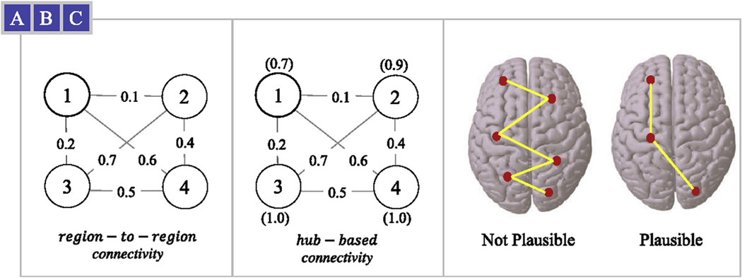
A particular challenge has been the identification of personalized structural connectivity patterns in connectome data, commonly known as fingerprints, given the high variability of network configurations across individuals. Hence, this is a problem best suited for machine learning algorithms given the richness and the complexity of whole brain connectivity. Machine learning applied to the connectome can attempt to learn connectivity patterns in a variety of ways. On the one hand, it can focus on region-to-region connectivity information (Fig. 1A), which represents a local measure of connectivity by focusing on two connected brain regions at a time. On the other hand, machine learning can learn patterns derived from hub-based network analysis (Fig. 1B), taking into consideration regional or global network topology¹ in an abridged way. The latter are important components of the connectome as they can overcome the limitations of assessing only node or edge properties of indirect paths between regions, which depict an incomplete assessment of the brain’s network. To overcome this problem, Mišić et al. recently reported a novel approach to best evaluate connectome properties by measuring dynamic spreading models (Mišić et al., 2015). By considering direct and indirect patterns of information spread, connectome dynamics have the potential to unravel more complex pathways and better model the latent properties of neural network architecture. To date, connectome dynamics, which may provide a better assessment of the properties and clinical translational potential of core individual neural network configurations, have not been used to assess personalized fingerprints.

Fig. 1.

Example connectivity based on (A) region-to-region values (e.g. in graph terminology the weight of an edge that connects two nodes), and (B) hub-based values, i.e. the Eigenvector centrality measure annotated in parenthesis above or below the node. (C) Using region-to-region values in Dijkstra’s single source shortest path may not be biologically plausible solution, however when region-to-region and hubness values are combined (our proposed dynamic) a more plausible shortest path solution may be found.

Existing studies using a structural or functional connectivity fingerprint have reported the ability to recognize the identity of a person (Finn et al., 2015; Yeh et al., 2016), predict cognitive or motor skill development (Finn et al., 2015; Liu et al.; Kawahara et al., 2017; Ball et al., 2015; Girault et al., 2019), or even the intelligence quotient (IQ) based on morphometric connectivity technique (Seidlitz et al., 2018). Nonetheless, it remains unclear whether a critical set of structural subnetworks are important for cognitive development from childhood to adult years. More specifically, do fingerprints depend on a set of core subnetworks that remain important from childhood to adulthood, and can they be used to estimate various personalized variables such as individual cognitive performance or neurodevelopment over different age demographics with a high degree of accuracy? In this study, we specifically tested whether connectome dynamics could identify linked brain regions constituting a structural subnetwork whose properties: a) can serve as a personalized structural brain fingerprint used to tell individuals apart, and b) relate to individualized behavioral performance. We hypothesize that connectome dynamics could contribute to the development of neural network individuality, developmental trajectories, and neuropsychological profiles.

To fully assess connectome dynamics, we propose a novel approach that leverages the technique introduced by Mišić et al. in which hub regions are likely to shape communication pathways. In particular, node hubness information is included in Dijkstra’s single-source shortest path algorithm (Cormen et al., 2009) to identify subnetworks that form these core communication pathways. By assessing connectome dynamics that take into account node hubness, rather than region-to-region information, we propose that indirect and direct pathways can be fully accounted for, while also incorporating the influence provided by nodes that act as hubs, which likely have a profound influence in orchestrating neuronal communication (Mišić et al., 2015) and determining functional properties (i.e., relate to cognition). We propose that the resulting connectome dynamic will thus be a shorter, simpler, communication path representing a more biologically plausible solution (Fig. 1C). Using a data-driven approach, i.e., no prior anatomical or clinical assumptions, we used deep learning to detect and test whether our connectome dynamics approach could accurately recognize the identity of a person and do so with higher classification accuracy than single-measure edge weight or hub-based approaches alone. Lastly, we test if our connectome dynamic characteristics could reliably predict individual performance in childhood (neurodevelopment) and adulthood (intelligence quotient).

2. Materials and methods

2.1. Person identification dataset

Twenty adult participants with no history of neurological or psychiatric disorder were included in this MRI study that was approved by the Institutional Review Board at the University of Göttingen. Each participant underwent three separate MRI study scans at the University of Göttingen in Germany, and the number of males and females were 8 and 12, respectively. The mean age at the first scan was 34.6 years (SD = 10.7). The second scan session was performed using the same scanner as the first session, and had the exact same scan parameters (SI Appendix: MRI scan parameters). On average, the second scan was 126.4 (SD = 102.8, range 12–442) days after the first scan. Lastly, the third scan session was performed in a different scanner, however employed the same scan protocol as the first and second. On average, the third scan was 158.4 (SD = 103.6, range 21–465) days after the first scan.

2.2. Early learning dataset

One hundred and forty-one children were included in this study. All children underwent MRI scans (SI Appendix: MRI scan parameters) and received a cognitive assessment at age two using the Mullen Scales of Early Learning that was approved by the University of North Carolina at Chapel Hill’s Institutional Review Board. Their mean age at image scan was 27 months (SD = 29 weeks), the maximum achievable cognitive assessment score was 150, and the number of males and females were 85 and 56, respectively. Cognitive ability was assessed at age two using the Mullen Scales of Early Learning (MSEL). Child measures of fine motor, visual reception, expressive and receptive language were collected by experienced testers. Age-standardized T-scores from these four scales were combined into an Early Learning Composite (ELC) standardized score (range: 49 to 155, mean = 100, SD = 15). The ELC has high internal consistency (median = 0.91) and reliability (median = 0.84 for the cognitive scales during these testing ages), and principal factor loadings of the scales lend support for the construct validity of the ELC as a general measure of cognitive ability, much like an intelligence quotient.

2.3. IQ dataset

Fifty-eight participants with no history of neurological or psychiatric disorder were included in this study after signing an informed consent that was approved by the Institutional Review Board at the Medical University of South Carolina. Their mean age at image scan (SI Appendix: MRI scan parameters) was 54.7 years (SD = 8.7), the maximum achievable IQ score was 128.7, and the number of males and females were 13 and 45, respectively. All the participants underwent verbal performance assessment using the North American Adult Reading Test Revised version (NART-R) as an estimator of IQ levels and intellectual function. Verbal intelligence was calculated in accordance with the NART-R as: Estimated Verbal Scale IQ = 128.7–0.89 x NART-R errors.

2.4. Structural connectome

The following steps were used to build each participant’s connectome using an automated connectome processing pipeline (or connectome pipeline for short) that sequentially performed the following steps: (i) segmented the T1-weighted images using SPM12’s unified segmentation-normalization process to determine the probabilistic grey matter (GM) and white matter (WM) maps; (ii) divided the probabilistic GM map into $m=83$ cortical and subcortical anatomical regions (or ROIs) based on the Lausanne anatomical atlas (SI Appendix: Supplementary Table S1); (iii) registered the WM and GM parcellation maps into the DTI space; (iv) computed GM pairwise probabilistic DTI fiber tracking; Probabilistic tractography was performed using each of the $m$ cortical ROIs in the diffusion space as the seed region by the FMRIB Diffusion Toolbox (FDT) probabilistic method (Behrens et al., 2007) with FDT’s BEDPOST being used to build default distributions of diffusion parameters at each voxel, followed by probabilistic tractography using FDT’s probtrackX. To minimize motion artifacts, our automated pipeline incorporated well known QC protocols (Andersson et al., 2003, 2016) that detected slice-wise and gradient-wise intensity and motion artifacts, replaced gradients of poor quality, and then corrected for motion and eddy current effects. Lastly, to reduce undetected connectome failures, visual QC checks were manually performed to ensure GM and WM surfaces were properly registered to the DTI space. A whole-brain connectivity matrix, or connectome, was constructed using results of step (iv). More specifically, connectivity was measured by the number of probabilistic white matter (WM) fiber tract streamlines arriving at ROI $j$ when ROI $i$ was seeded, averaged with the number of probabilistic WM fiber tract streamlines arriving at ROI $i$ when ROI $j$ was seeded. This step was iteratively repeated to ensure all 83 ROIs were treated as seed regions resulting in a symmetric $mxm$ connectivity matrix $C$, where $C(i,j)$ was the weighted undirected network connection between ROIs $\text{i}$ and $\text{j}$. Note that since the number of streamlines are averaged between each ROI, $C$ is symmetric with respect to the main diagonal, i.e., $C(i,j)=0$ when $i==j$.

2.5. Connectome dynamic

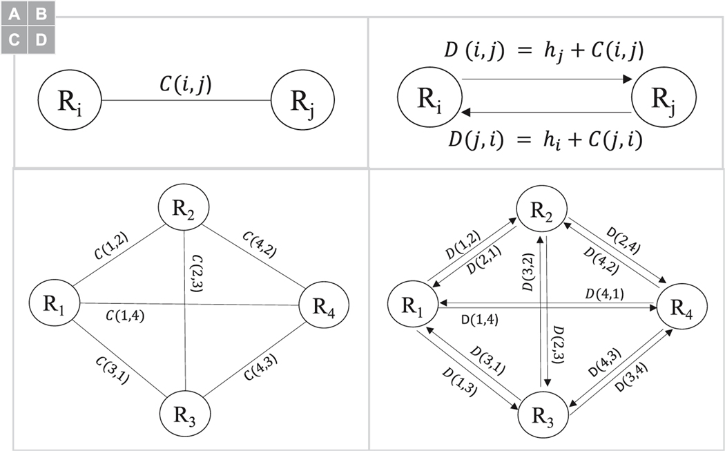
Before the proposed connectome dynamic can be computed, region-to-region connections and region hubness measures are combined using a simple, and straight forward, approach that turns an undirected region-to-region connection (Fig. 3A) to a pair of hub-directed connections (Fig. 3B). In a grapth-theoretic sense, a weighted undirected graph (Fig. 3C) is converted to a weighted directed graph (Fig. 3D). In particular, given a $mxm$ undirected and symmetric connectivity matrix $C$, a $mxm$ directed non-symmetric connectivity matrix $D$ is constructed using the sequence of steps provided below.

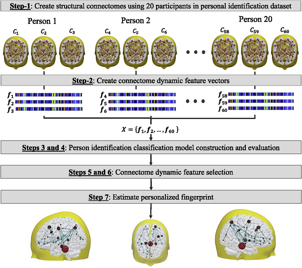
Fig. 3.

Overall approach to estimate the personalize fingerprint using the connectome dynamic vectors of the 20 participants in the personal identification dataset. In general, seven sequential steps are performed to estimate the personalized fingerprint.

1. First a set of ROI hubness values $\text{H}={\left\{h_i\right\}}_{i=1}^m$ was computed using the undirected connectivity values in $C$, where $h_i$is the hubness measure for ROI $I$ that is calculated using one of three hub-based graph-theoretic measures (SI Appendix: Hubness measures).

2. The undirected WM connection $C(i,j)$ between ROIs $i$ and $j$ (Fig. 3A) was converted into a pair of directed connections using $C(i,j)$ and ROI hubness values $h_i$ and $h_j$ (Fig. 3B). Specifically, $D(i,j)=h_j+C(i,j)$ and $D(j,i)=h_i+C(j,i)$, where direction is encoded using the hubness value of ROI $b$ in the $(a,b)$ 2-tuple.

3. Step-2 was repeated for each $i$ and $j$ in $C$.

Next, an $N=m(m\text{-1)}$ dimension connectome dynamic vector $f\text{=}\left(f_1,\dots ,f_{\alpha },\dots ,f_N\right)$ was created by applying Dijkstra’s single source shortest path algorithm to the $mxm$ directed non-symmetric connectivity matrix $D$, where $\alpha =(s,e)$ is an index $(\alpha )$ to 2-tuple $(s,e)$ mapping that defined the source $\left(s\right)$ and destination $\left(e\right)$ ROIs that were provided to the shortest path algorithm with $s\ne e$. Importantly, since the single source shortest path algorithm can be applied to a directed graph, the connectome dynamic vector can be found without any modification to the shortest path algorithm. Since most, to all, versions of Dijkstra’s algorithm find the minimum shortest path, i.e. path with the least cost, the inverse value was computed for each element in D that had a value greater than zero. Furthermore, the natural logarithm² was also applied to the inverse values in D to ensure, as best as possible, the underlying distribution of directed network connections was normally distributed before the algorithm is ran. After algorithm completion, smaller dynamic connectome feature values where converted to larger ones, and vice versa, by taking the inverse of each feature value in $f$. This step is necessary because the person identification classification model (Section 2.6) applies a supervised learning approach that required larger input feature values.

2.6. Personalized fingerprint

The overall approach (Fig. 3) used to estimate the personalized fingerprint is outlined in the seven-step procedure below. It is important to note, even though each feature in the connectome dynamic vector represented a path between two different ROIs in the brain, in the context of this study, were refer to each pair of ROIs as subnetwork. Here, the definition of subnetwork is not related to the nine well-known resting-state functional networks (van den Heuvel et al., 2009) or based on pre-existing neuroanatomy brain network models. Rather, the sub-networks found by our connectome dynamic modeling approach (detailed in Step-7) were purely graph-theoretic and not biological in nature. Since Dijkstra’s algorithm was used to find the shortest path, the resulting subnetwork could represent a single edge that connected two different brain regions, i.e. no intermediate brain regions are in the path between the source and destination brain regions.

1. A set of connectomes $C={\left\{C_i\right\}}_{i=1}^n$ was created (Section 2.4) using each participant image scan in the person identification dataset (Section 2.1). Since each participant had three image scans, the total number $\left(n\right)$ of connectomes was sixty (20 participants x 3 scans = 60 connectomes). For the supervised learning process a set of participant identity labels $Y={\left\{{\mathit{y}}_{\mathit{i}}\right\}}_{i=1}^n$ was also created, where $y_i$ is a 20-dimension binary label vector that defined the participant binary label for connectome $C_i$. For example, binary label vectors $y_1$, $y_2$, and $y_3$ would be (1, 0, 0, 0, 0, 0, 0, 0, 0, 0, 0, 0, 0, 0, 0, 0, 0, 0, 0, 0) for participant one connectomes $C_1$, $C_2$, and $C_3$.

2. A set of connectome dynamic feature vectors $X={\left\{f_i\right\}}_{i=1}^n$ was estimated (Section 2.5) for each connectome in $C$.

3. The input feature data $\left(X\right)$ and the label data $\left(Y\right)$ were used to construct deep-learning $\left(\text{DL}\right)$ a person identification model (SI Appendix: Neural network architecture). In general, the person identification model had one input (a connectome dynamic feature vector) and twenty outputs (one for each participant in the person identification dataset).

4. Person identification model performance was evaluated using a three-fold cross-validation strategy that incorporated a two-dimension grid search procedure which was used to identify the optimal momentum and learning rate neural network parameters. In particular, three-folds were selected because each adult participant had three different connectome dynamic vectors, (i.e. first fold had 20 connectome dynamic vectors, one for each participant in the first scan session; second fold has 20 connectome dynamic vectors, one for each participant in the second scan session; and the third fold has 20 connectome dynamic vectors, one for each participant in the third scan session). Thus, two vectors were used to train the model and the remaining unseen vector was used to test the model. For each connectome dynamic vector, in each test fold, classification accuracy was evaluated using the known participant labels, where a score of 100% meant the identity of all twenty participants were correctly recognized (Section 3.1: Person identification classification performance).

5. For each person identification model generated by the 3-fold evaluation process, the neural network backtrack technique (Girault et al., 2019) was applied to identify which input connectome dynamic features had the greatest contribution to classification accuracy. In particular, after the backtrack technique was applied to a trained person identification model, each feature in the connectome dynamic vector was assigned a normalized backtrack contribution weight value in the [0 1] range, where a value of one implied the feature had the greatest contribution to classification accuracy. Lastly, the three normalized backtrack contribution weight value results (for the three trained models) where then averaged to produce the final backtrack contribution weights values (Section 3.2: Connectome dynamic feature selection).

6. Unfortunately, because the number of input connectome dynamic features was very large, the number of non-zero contribution weight values was also very large, i.e. even though more than 75% of the weight values were zero, the number of non-zero weight values would still be in the thousands, which is not desirable. To further reduce the number of non-zero backtrack contribution weights found int Step-5 above, an iterative feature reduction approach (SI Appendix: Iterative feature reduction approach) was additionally performed to identify the optimal number of connectome dynamic features $\left(k\right)$ that had the greatest influence on classification accuracy (Section 3.2: Connectome dynamic feature selection).

7. The $k$ optimal connectome dynamic features selected in Step-6 were converted back into the subnetwork $\left(S\right)$ path originally identified by single source shortest path algorithm. Next, a majority vote technique (Fig. 4) was applied to find the majority subnetwork $(\widehat{S})$ across all participants in the person identification dataset. This step was required because, even though the source and destination brain region were the same for one particular connectome dynamic feature, both the number of brain regions along the subnetwork path (i.e. path length), and the specific brain regions along the subnetwork path were likely to differ by a small amount across all the participants. Finally, the personalized fingerprint $F={\left\{{\widehat{S}}_i\right\}}_{i=1}^k$ is formed that defines the $k$ majority subnetworks (Section 3.3: Personalized fingerprint).

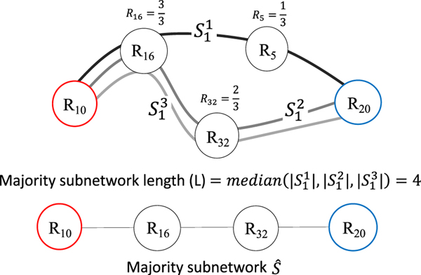
Fig. 4.

Example that illustrates how we estimate the majority subnetwork. Given a small dataset of $n=3$ participants ${\left\{S_1^i\right\}}_{i=1}^n$ for subnetwork $S_{\text{1}}$ that begins at ROI 10 (red) and ends at brain ROI 20 (blue), the majority subnetwork path length $L$ is found where $\text{|}S\text{|}$ is the number of ROIs (including start and end). Next, the remaining intermediate ROIs that have the greatest occurrence are identified, e.g. ROI 32 is in two of the three subnetworks so the occurrence value is 2/3. The top intermediate brain region occurrence values are thus selected and then combined with the begin and end ROIs to form the majority subnetwork $\widehat{S}$. Note: R is short for ROI in the above illustration.

2.7. Personalized fingerprint and percent whole brain WM connectivity

The total amount of fingerprint WM connectivity ${\text{T}}_{\text{S}}$ s found by

$${\text{T}}_{\text{S}}=\sum _{\forall \text{p}\in \text{p}}\sum _{\widehat{\forall S}\in \text{F}}\text{f}\left({\text{C}}_{\text{p}}(\widehat{\text{S}})\right),$$ Eq.1

where $P$ is a set of study participants, $F$ is the personalized fingerprint, $C_p$ is the connectome for participant $P$, and $\text{f}(\cdot )$ is a function that sums the region-to-region connections in $C_p$ that make up majority subnetwork $\widehat{S}$. It is important to point out, does not include any hubness information, just white matter connectivity. The total amount of whole brain WM connectivity ${\text{T}}_{\text{W}}$ is found by

$${\text{T}}_{\text{W}}=\sum _{\forall \text{p}\in \text{P}}\mathrm{striu}\left({\text{C}}_{\text{p}}\right),$$ Eq.2

where $striu(\cdot )$ is a function that sums the region-to-region WM connections in the upper triangular portion in $C_p$ not including the diagonal. Lastly, the fraction of fingerprint WM connectivity to whole brain connectivity is ${\text{T}}_{\text{S}}/{\text{T}}_{\text{W}}$ (Section 3.5: Personalized fingerprint and percent whole-brain WM connectivity).

2.8. Personalized fingerprint and cognitive prediction modeling

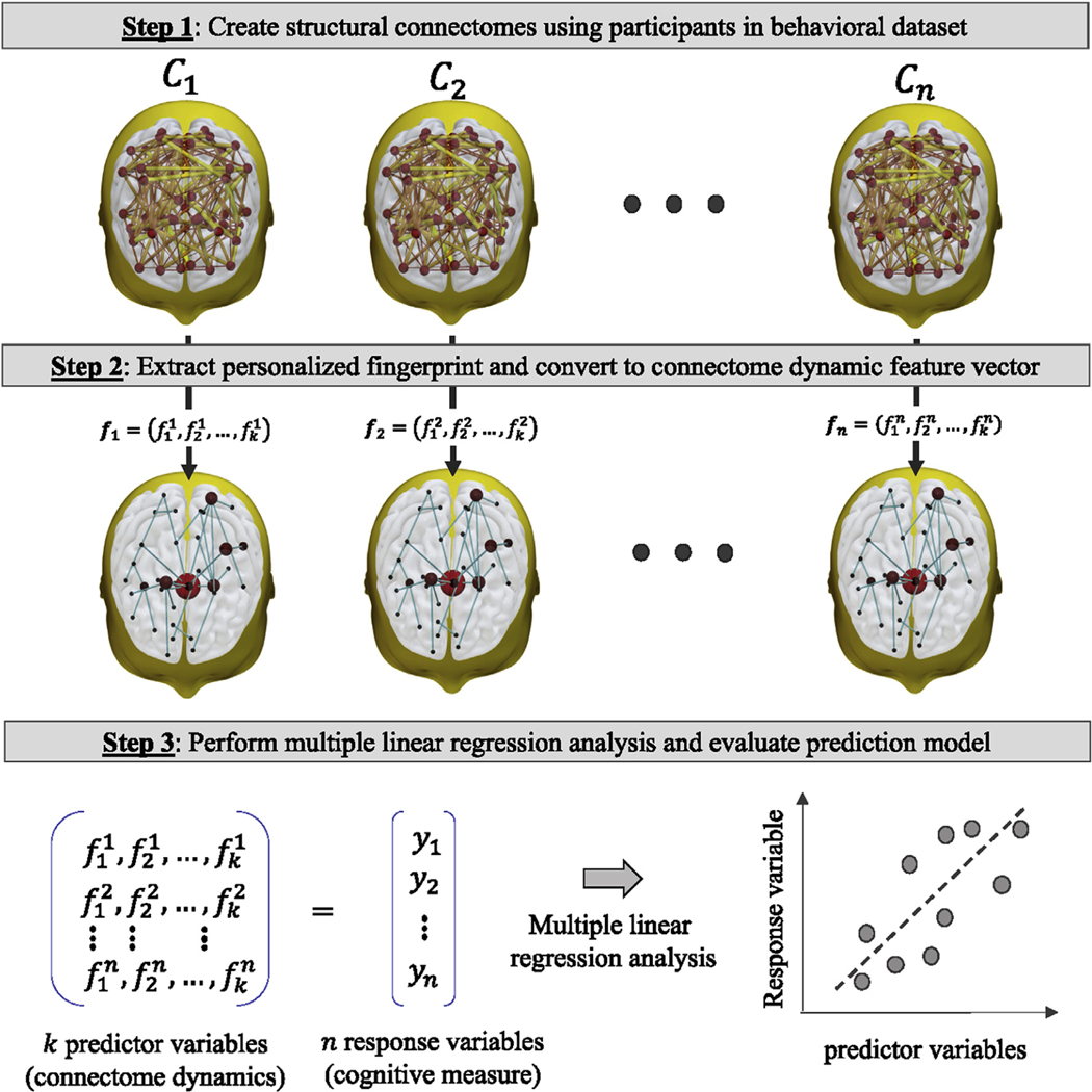
To demonstrate that person identity classification accuracy was independent of dataset employed and demographic population the personalized fingerprint (Section 2.6) was applied to a connectome dataset and then used to predict individual cognitive performance (Fig. 5). In general, the prediction modeling approach is outlined below.

Fig. 5.

Prediction modeling approach to evaluate the relationship between personalized fingerprint connectome dynamics and cognitive measures of two different age demographics (i.e. early learning composite score in sample of toddlers, and IQ in a sample of adults).

1. A set of connectomes $C={\left\{C_j\right\}}_{j=1}^n$ was created (Section 2.4) using each participant image scan in a cognitive dataset (Section 2.2 Early learning dataset; Section 2.3 IQ dataset), where $n$ is the total number of participants. A response variable vector $y=\left(y_1,y_2,\dots ,y_j,\dots ,y_n\right)$ was also created, where $y_j$ is the cognitive measure (ELC or IQ) for participant $j$.

2. The ROI hubness values ${\left\{h_i\right\}}_{i=1}^m$ for connectome $C_j$ was computed, and then for each majority subnetwork $(\widehat{S})$ defined in the personalized fingerprint (Section 2.6: Step-7), a $k$-dimension fingerprint connectome dynamic vector $f_j=\left(f_1^j,f_2^j,\dots ,f_k^j\right)$ was created. Specifically, connectome dynamic feature $f_i^j=\sum _{\forall (a,b)\epsilon S_i}{h}_b+C_j(a,b)$, where $(a,b)$ is a connection between ROIs $a$ and $b$ in majority subnetwork ${\widehat{S}}_i$. This step is repeated for each connectome in $C$.

3. Multiple linear regression was then applied to a $n\times k$ dimension predictor variable matrix (created with the $n$ fingerprint connectome dynamic feature vectors) and the response variable vector $y$. For the early learning prediction model, the dependent variable was the 2-year ELC score, and for the IQ prediction model the dependent variable was the IQ score. The prediction accuracy of both models was evaluated using a leave-one-out cross-validation procedures and the absolute error measure (Section 3.4: Personal fingerprint and cognitive prediction performance).

2.9. Anatomo-functional contextualization

We employed the decoder method in Neurosynth (Yarkoni et al., 2011) to evaluate the functional loadings of each anatomical atlas region composed in each majority subnetwork (Section 2.6) in relationship to broader cognitive search terms, such as: memory, motor, language, vision, visuospatial, taste, disgust, emotion, auditory, pain, somatosensory, conflict, conditioning, switching and inhibition. The result was a Pearson correlation between each region, NIFTI images in the person identification dataset were coded as one for the voxels in the ROI, and zero elsewhere, and the reverse inference meta-analysis functional map, i.e., the probability map of regional activation given the cognitive term. Of course, this is an artificial correlation since all regions were input as one. Nonetheless, they represent a weighted measure of functional loadings. The resulting values (Section 3.3, Fig. 8) were normalized in a min-max scaling approach per each majority subnetwork Section 3.3, Fig. 7) and their anatomo-functional contextualization (Supplementary Table S2).

Fig. 8.

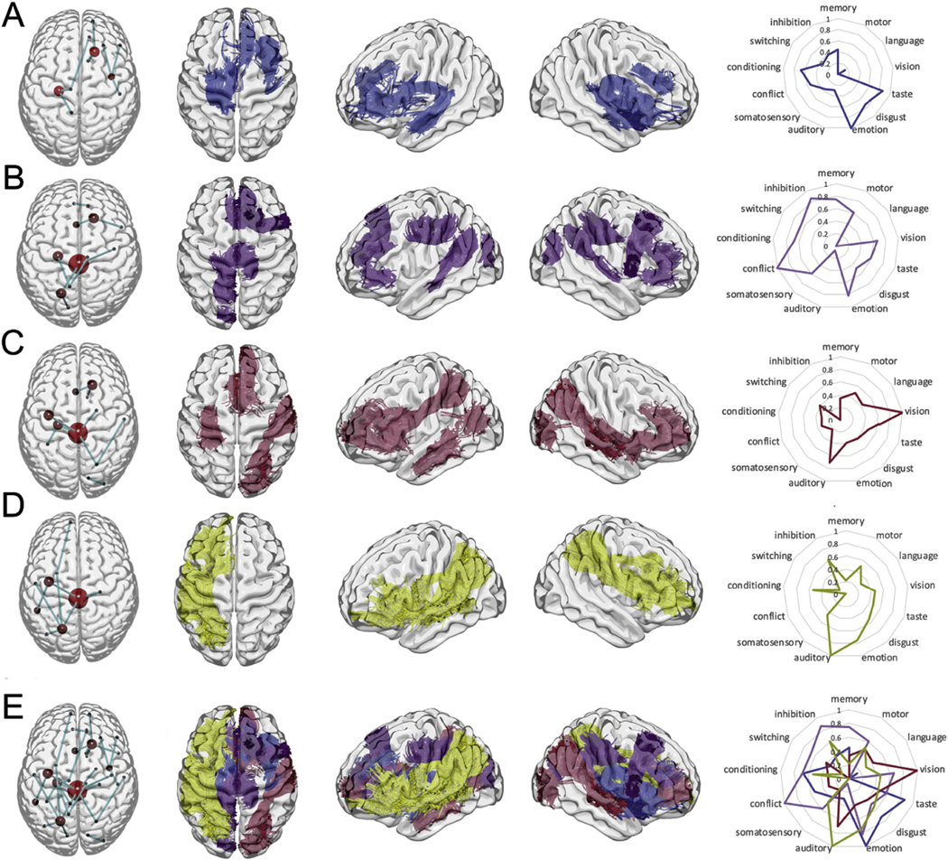
Individual subnetworks formed by the top (A) 1-to-4, (B) 5-to-8, (C) 9-to-12, and (D) 13-to-16 majority subnetworks, shown grouped together in (E). The first columns demonstrate the schematic location of brain regions and connections, whereas columns 2 to 4 demonstrates the locations of white matter tracts representing the same connections. For clarity, the connections to the brain stem are not included in columns 2 to 4. The right-most column demonstrates functional loadings to the nodes in each subnetwork based on reverse inference maps from a large database of functional imaging studies included in Neurosynth (Yarkoni et al., 2011). Note: brain regions are represented by red nodes and the size of the node is the related to the number of times the brain region is present in one, or more, majority subnetworks.

Fig. 7.

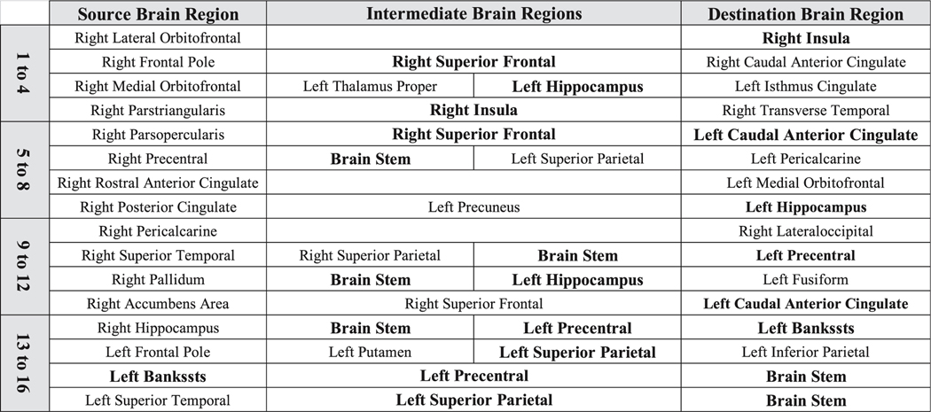
The top 16 majority subnetworks that form the personalized fingerprint, categorized in to groups of four. Table cells with bold font indicate brain regions that are present in more than one majority subnetwork. Bankssts refers to the cortical areas around superior temporal sulcus.

3. Results

3.1. Person identification classification performance

The classification accuracy of the deep-learning (DL) person identification models (Section 2.6; Step-3) were evaluated and then compared to the classification accuracy of linear multi-class support vector (SV) person identification models (Table 1). The optimal model parameters found by the 3-fold grid search procedure (Section 2.6; Step-4) that yielded the highest accuracy were: momentum set to 0.5 and learning-rate set to 0.001 for DL models, and regularization penalty ($C$) set to 0.75 for SV models. Additionally, the same optimal model parameters values were used to train DL and SV person identification models that used hub-only, region-to-region, and existing dynamics measures. Using the optimal model parameters, the 3-fold process was repeated twenty times (to assess the stability of our modeling approach) and the reported classification accuracy was computed by finding the mean and standard deviation of the sixty test folds (i.e. 3-fold process executed twenty times results in sixty test folds).

Table 1.

Comparision of person identification model performance using two different machine-learning approaches: deep-learning (DL) and multi-class support vector (SV) based on a linear kernel³. Both modeling approaches were evaluated using different connectome features (i.e. proposed connectome dynamic, graph theoretic measures, WM region-to-region connectivity, and existing dynamics based on graph topology).

Connectome Feature	Deep learning (DL) classification model		Support vector (SV) classification model
	Mean	SD (±)	Mean	SD (±)
Proposed dynamic (Section 2.5)
Directed shortest path using eigenvector centrality hub measure	93%	4%	72%	7%
Directed shortest path using betweenness centrality hub measure	92%	6%	71%	9%
Directed shortest path using clustering coefficient hub measure	89%	6%	69%	9%
Graph theoretic hubness measure (SI Appendix)
Betweenness centrality	65%	9%	45%	10%
Eigenvector centrality	65%	9%	47%	11%
Clustering coefficient	57%	7%	48%	10%
WM connectivity (Section 2.4)
Region-to-Region	41%	12%	44%	11%
Existing dynamics based on graph topology
Communicability (Yarkoni et al., 2011)	60%	7%	49%	10%
Mean first passage time (Estrada and Hatano, 2008)	66%	8%	42%	9%

The classification accuracy of DL and SV person identification models were evaluated using different connectome features, specifically: 1) proposed connectome dynamic features (Section 2.5), 2) hubness only features (SI Appendix: Hubness measures), 3) region-to-region WM connectivity features (Section 2.4), and 4) graph topology dynamic features based on region-to-region communicability⁴ (Estrada and Hatano, 2008) or mean first passage time⁵ (Goñi et al., 2013).

Independent of the machine-learning algorithm (DL vs. SV), the reported classification accuracies (Table 1) suggest that person identification models that use our connectome dynamic provides a richer descriptor of subtle brain network pathway differences that are likely intrinsic to a particular individual. More specifically, compared to person identification models that use simple features such as WM region-to-region connectivity (Section 2.4) or region hubness (SI Appendix: Hubness measures), or more complex features such as communicability or mean first passage time, the classification performance of models that use our connectome dynamic feature were, on average, ~26% more accurate than models that used hubness, communicability, or first mean passage time features, and ~39% more accurate than models that used region-to-region features.

When considering machine-learning algorithm, DL person identification models were, on average, ~18% more accurate than SV person identification models. Furthermore, DL person identification models that used our connectome dynamic were, on average, ~21% more accurate than SV models that used our connectome dynamic. Lastly, DL person identification models that used connectome dynamic features were, on average, ~33% more accurate than models that used communicability features and ~24% more accurate than models that used mean first passage time features.

Furthermore, DL person identification models that use connectome dynamic features were, on average, 91% accurate. By contrast, DL models based solely on region-to-region connections, hub-based features, or topological features were, on average, 41%, 62%, or 63% accurate, respectively. Among the connectome dynamic approaches that incorporate brain region hubness in the dynamic calculation (Section 2.5), Eigenvector centrality yielded the highest classification accuracy.

Lastly, since the connectomes in the person identification dataset (Section 2.1) were acquired on two different MRI scanners, the reported classification accuracies (Table 1) suggest that for our modeling approach (that uses connectome dynamic features) there is little to no discrepancy in classification accuracy between the two MRI scanners. If scanner discrepancies did exist, the mean accuracy would likely be 67%, that is, the third participant connectome (acquired on a different scanner) would be consistently misclassified. However, the reported mean accuracy for our highest performing connectome dynamic, that used Eigenvector centrality hubness, was ~93%, and the mean accuracy for our lowest performing connectome dynamic, that used clustering coefficient hubness, was ~89%.

3.2. Connectome dynamic feature selection

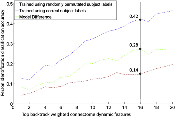
Our connectome dynamic feature selection approach was applied to the sixty person identification models (3-fold cross-validation procedure repeated twenty times) that used the connectome dynamic with the highest mean classification accuracy, specifically, connectome dynamic features that included Eigenvector centrality hubness in the dynamic calculation. Specifically, the backtrack technique generated a final backtrack contribution weight vector (Section 2.6; Step-5) that reduced the number of connectome dynamic features from $N=6806$ features to 1384 (~79% reduction). Next, our iterative approach (Section 2.6; Step-6) was then applied to the final backtrack contribution weight vector to further reduce the number of connectome dynamic features from 1384 to $k\text{=16}$ (~98% reduction) (Fig. 6).

Fig. 6.

Results of iterative feature reduction approach. At each iteration, the top final backtrack weighted connectome dynamic features were used to train neural networks with the correct participant labels, and to train neural networks with randomly permutated participant labels. At each iteration the difference in classification accuracy is recorded, and the greatest difference was achieved when the top $\mathit{k}=16$ connectome dynamic features are used.

3.3. Personalized fingerprint

The top $k\text{=16}$ connectome dynamic features that incorporated the Eigenvector centrality hubness measure in the dynamic calculation were converted back into the original shortest path found by single source shortest path algorithm, and then the sixteen majority subnetworks were found (Section 2.6; Step-7). The brain regions involved in each of majority subnetworks were categorized into quartiles (Figs. 7 and 8), namely, the top 1-to-4 (Q1), 5-to-8 (Q2), 9-to-12 (Q3), and 13-to-16 (Q4). Overall, top majority subnetworks involved both ipsilateral and contralateral connections mostly, but not exclusively, involving frontal and temporal lobes as well as regions throughout the parietal and occipital regions typically playing an associative role. In addition, cortico-subcortical links were noted. The relationship between the brain regions identified in the top sixteen majority subnetworks and a meta-analytic compendium of functional reverse inference maps was also performed (Fig. 7 right most column). The average functional loading for the brain regions in each majority subnetwork grouping is shown (next to the anatomical connectivity paths). All functional loadings were normalized to facilitate visualization (Section 2.9: Anatomo-functional contextualization). In summary, Q1 had higher loadings on emotion, taste and conditioning, Q2 on conflict and inhibition, Q3 on vision and auditory processing, and Q4 on auditory and emotional functions.

3.4. Personalized fingerprint and percent whole-brain WM connectivity

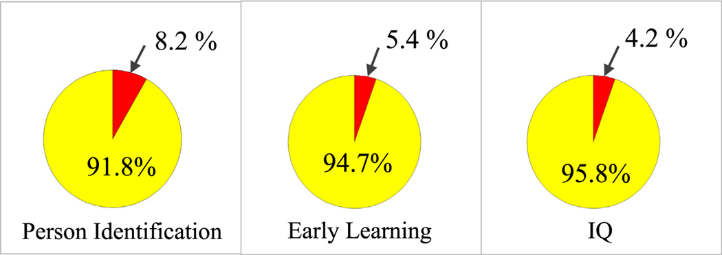
The relationship of WM connectivity in the entire brain to the WM connectivity in the 16 majority subnetworks that form our personalized fingerprint (Section 3.3, Fig. 7) was also analyzed. Using Eqs. (1) and (2) (Section 2.7), for the sixty adult connectomes in the person identification dataset, approximately 8.2% of all the WM connectivity in the entire brain is expressed in the personalized fingerprint (Fig. 9). For the one hundred and forty-one toddler connectomes in the early learning dataset approximately 5.4% of all the WM connectivity in the entire brain is expressed in the personalized fingerprint (Fig. 9), and for the fifty-eight adult connectomes in the IQ dataset approximately 4.2% of all the WM connectivity in the entire brain is expressed in the personalized fingerprint (Fig. 9).

Fig. 9.

Total white matter (WM) connectivity percentages. The “red” shows the percent WM described by the personalized fingerprint when applied to the following connectome datasets: person identification, early learning, and IQ. The “yellow” is the total ROI-to-ROI WM percentage minus the WM fingerprint percentage.

3.5. Personalized fingerprint and cognitive modeling performance

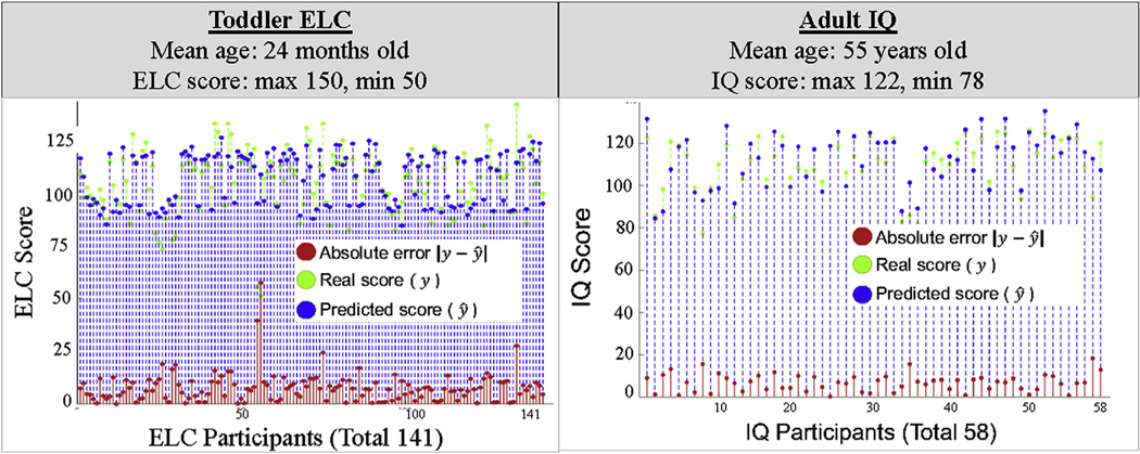
Using the 16 majority subnetworks that form our personalized fingerprint (Section 3.3, Fig. 7), and our predictive modeling approach (Section 2.8, Fig. 5), early learning 2-year prediction LOOCV mean absolute error was 7.7 points $(\text{SD}=7.1)$ (Fig. 10; Toddler ELC), and the mean correlation coefficient of the one hundred and forty-one prediction models created by the LOOCV procedure was 0.70$\left({\text{R}}^2=0.49,\text{SD}=0.16\right)$. The validity of our predictive modeling approach was also assessed by creating incorrect connectome dynamics derived from one hundred and forty-one toddler connectomes that had randomized⁶ connections (Maslov and Sneppen, 2002). The LOOCV procedure was repeated on the randomized connectomes and the mean absolute error was 22.1 points $(\text{SD}=11.8)$, and the mean correlation coefficient was 0.14$\left({\text{R}}^2=0.02,\text{SD}=0.08\right)$.

Fig. 10.

Toddler ELC and adult IQ model results. The ELC and IQ models were constructed and evaluated only using the $k=16$ majority subnetworks that form the personalized fingerprint.

Similarly, using the 16 majority subnetworks that form our personalized fingerprint, and our predictive modeling approach, the IQ prediction model LOOCV mean absolute error was 4.1 points (SD = 6.8) (Fig. 10; Adult IQ), and the mean correlation coefficient of the fifty-eight prediction models created by the LOOCV procedure was 0.76 (R² = 0.58, SD = 0.12). Likewise, the LOOCV procedure was repeated on the randomized connectomes and the mean absolute error was 24.3 points (SD = 0.6), and the mean correlation coefficient was 0.10 (R² = 0.01, SD = 0.05).

In addition to LOOCV, a 10-fold approach was also performed, and the 10-fold mean absolute prediction error for both the ELC and IQ models was within ±0.12 points, and the SD was within ±0.26 of the LOOCV mean absolute prediction error results. This suggests predictive models constructed with connectome dynamics derived from our personalized fingerprint were not dependent on the cross-validation procedure.

4. Discussion

This study sought to explore whether machine-learning could accurately identify individuals based on their structural brain connectivity and their behavioral performance. We demonstrated that models based on unique dynamic properties within specific brain networks are capable of singling out individuals and also predict cognitive development during childhood and IQ during adulthood with fairly high accuracy. Overall, our findings indicate that a personalized fingerprint in the brain is formed by a core set of sixteen subnetworks, is sufficient for differentiation between individuals, and can predict individual differences in intellectual development and function. To our knowledge, this is the first fingerprinting study to successfully predict personalized identity but also behavioral performance, such as individual identity and/or neurodevelopmental measure, in longitudinal image scan data collected at separate sites.

4.1. Whole-brain data-driven approach

In contrast with other connectome fingerprinting approaches that limit their analysis to a core set of known brain regions or subnetworks defined a priori, our data-driven approached used whole-brain connectivity to guide fingerprint construction. In doing so, the core set of sixteen subnetworks that form our personalized fingerprint (Figs. 7 and 8) were not based on prior knowledge or pre-assumptions. For instance, Yeh et al. (2016) identified a structural connectome fingerprint that demonstrates the highest classification accuracy based on connectivity localized to the corpus callosum, a known fiber-dense brain region. Using functional data, Finn et al. (2015) proposed a functional connectome fingerprint that demonstrates the highest classification accuracy, roughly 99%, when the approach was based on two well-known functional subnetworks that are localized to the medial frontal and frontoparietal brain regions. More recently, Liu et al. (Liu et al.) employed a sliding time-window approach to resting state functional MRI time-series data to pinpoint highly localized spatial patterns capable of identifying individuals with approximately 90% accuracy.

4.2. Neurodevelopment

A handful of connectome fingerprint studies (Finn et al., 2015; Kawahara et al., 2017; Ball et al., 2015; Girault et al., 2019) have constructed individual neurodevelopment (cognitive or motor ability) models that show good prediction performance. For instance, Finn et al. (2015) applied their functional connectome fingerprint to predict fluid intelligence in adult participants, and Ball et al. (2015) focused entirely on structural connectivity (region-to-region connections) localized to the thalamus and cerebral cortex (thalamocortical) regions to predict a cognitive score at two years old. Similar to Ball’s work, Kawahara et al. (2017) developed a convolutional neural network to predict a cognitive score at eighteen months old using custom structural connectivity filters (e.g. edge-to-edge, edge-to-node, and node-to-graph) however, the topological patterns learned by these customized filters are still localized to a specific brain region or neighboring connections. More recently, Girault et al. (2019) was able to predict the cognitive ability of children at 2 years old with a two-step machine learning approach that used whole-brain structural connectivity information (region-to-region connections) from full-term infants. However, it is unknown if the infant connectome fingerprints developed in these studies (Finn et al., 2015; Kawahara et al., 2017; Ball et al., 2015; Girault et al., 2019) can be applied to adolescent, teenage, or adult structural connectome data to predict a neurodevelopment measure with some reasonable amount of accuracy. Our fingerprinting approach, that uses connectome dynamics, intends to overcome this limitation.

4.3. Imaging modality considerations

Even though great advances have been made in functional connectome fingerprint approaches (Finn et al., 2015; Liu et al.), some challenges typically posed by functional approaches are related to motion, width of the sliding windows, parcellation schemes, and global signal removal (Chai et al., 2012; Schölvinck et al., 2010). Structural network information, by comparison, is not organized with time or spatial alignment. Accordingly, data derived from diffusion sequences tends to be less confounded by hemodynamic changes typically affecting the BOLD signal such as sleep, cardiovascular changes, and other autonomic nervous system fluctuations (Wu and Marinazzo, 2016; Glover, 2011). In fact, core features of this study’s design were based previous work demonstrating that the structural connectome is more stable (and thus reproducible) across scanners and over time when focusing on probabilistic tractography, especially when considering graph theory measures that reflect the topology of the network (Bonilha et al., 2015). Lastly, even though the scan duration of diffusion sequences are typically shorter than functional sequences, a subject is likely to move, which can introduce motion confounds in the connectome data. However, well known diffusion data QC protocols (Andersson et al., 2003, 2016), including visual QC inspections, are incorporated our connectome pipeline (Section 2.4) to minimize the impact of motion artifacts.

4.4. Connectome dynamic

The performance of person identification models that used connectome dynamic features were compared to models that used two existing graph dynamic features, i.e. communicability and mean first passage time, that, like our connectome dynamic take into account the entire graph topology. And even though all three dynamics measure amount of neuronal communication along the WM pathway between two different GM ROIs, our connectome dynamic outperformed mean first passage time and communicability dynamics (Table 1). In general, there are two important methodology limitations that may contribute to the discrepancy in classification accuracy.

1. Mean first passage time and communicability are both undirected graph measures, where the pathway measurement between $(RO{I}_a,RO{I}_b)$ is equivalent to $\left(RO{I}_b,RO{I}_a\right)$ and $RO{I}_a\ne RO{I}_b$. Alternatively, our connectome dynamic is directed graph measurement (Section 2.4, Fig. 2) that is sensitive to hub-directed pathway differences.

2. Mean first passage time and communicability are estimating the mean undirected pathway occurrence or sum of all undirected pathway occurrences, respectively. Our connectome dynamic approach, on the other hand, does not perform a mathematical (average or sum) operation on potentially thousands of undirected pathway solutions. Instead, our dynamic uses a shortest-path graph algorithm that represents a unique and optimal directed pathway solution (Section 2.4).

Fig. 2.

Converting a weighted region-to-region undirected connectome edge to weighted directed connectome edge. (A) Example undirected edge weight $\text{C}(\text{i},\text{j})$ that connects ROI $i$ and $j$. (B) Example directed edge weight $D(\text{i},\text{j})=h_j+\text{C}(\text{i},\text{j})$ from ROI $i$ to ROI $j$ where $h_j$ is a graph theoretic hubness value for ROI $j$ and $C(\text{i},\text{j})$ is the undirected edge weight value. (C) an example weighted undirected graph (i.e. connectome), and (D) is the weighted directed graph that is used to calculate our connectome dynamic. Note: R is short for ROI in the above illustration.

These limitations may render the mean first passage time and communicability dynamics insensitive to subtle pathway differences that are capable of singling out individuals. More specifically, the desired dynamic properties should minimize: data smoothing operations (such as those introduced by an averaging operation) that may remove subtle pathway information, and pathway summation operations that may enhance noise artifacts. To better understand the desired properties of our connectome dynamic, a correlation analysis was performed (SI Appendix: Connectome feature correlation analysis) that suggests including hubness in the dynamic calculation will likely: reduce path-length (create shorter, simpler, pathways) and thus suppress noise artifacts, and enhance subtle pathway information by routing through highly connected pathways.

In addition to the individual-level sensitivity limitations listed above, for the graph dynamic modeling approach to be practical, the dynamic must represent a physical brain subnetwork (Section 2.6; subnetwork definition) that:

1. exists in a structural connectome (based on a known parcellation),

2. is universal, i.e. exists in the brain of all individuals,

3. is preserved across human development.

As outlined in (II) above, because mean first passage time and communicability dynamics are not unique and/or optimal, these two approaches would not satisfy (a,b), and would not be a suitable solution.

Obviously, (a,b) is dependent on a specific brain parcellation, however since our dynamic is a pathway found by the shortest path algorithm, (a) is satisfied because a simple and straightforward technique exists to convert our connectome dynamic to a unique subnetwork that is defined in the participant’s connectome. To satisfy (b), a simple majority analysis (Fig. 4) was on performed on each subnetwork then applied to each participant connectome in the dataset to identify a majority subnetwork for each subnetwork.

Satisfying (c) is more difficult, however existing studies (Baker et al., 2015; Ball et al., 2014; van den Heuvel and Sporns, 2011; van den Heuvel et al., 2015; Cao et al., 2016; Yap et al., 2011; Huang et al., 2015; Hagmann et al., 2010) that use various graph-theoretic approaches propose the existence of an underlying connectome blueprint in adults, children, and neonates alike. More importantly, Batelle et al. (Batalle et al., 2017) suggest that two types of structural connections exist in neonates: core connections that remain intact and largely unaltered even if born premature (<thirty-seven weeks gestational age), and local connections that are altered in premature neonates. Based on these existing studies, and since our dynamic modeling approach is able to predict person identity of adults with ~90% accuracy (Table 1), the real ELC score of a two-year-old toddler with ~7 points (Fig. 10), and the real IQ score of an elderly adult within ~4 points (Fig. 10), these results further support the practicality of our fingerprinting approach. More specifically, the core set of subnetworks that form our personalized fingerprint (Figs. 7 and 8) likely represent: simpler, shorter, pathways (as discussed above) that are present at birth, and likely remain unchanged across human development (Fig. 9).

4.5. Machine-learning algorithm

The choice of supervised machine-learning algorithm was also evaluated to determine its impact on model performance (Table 1), and in general, the classification accuracy of DL person identification models were better than SV person identification models. Interestingly, even though DL outperformed SV, the top twenty-five features found by DL backtrack technique (Section 2.6; Step-5) and the SV algorithm (i.e. support vectors that had the largest weight coefficients) were in agreement. Moreover, they were also in agreement for classification models that used our three dynamics (Eigenvector centrality, betweenness centrality, and clustering coefficient). This finding suggests why DL models have improved classification accuracy. In particular, when connectome dynamics are combined in a multiple-layer hierarchical (deep-learning) modeling approach, verse a single-layer (support vector) modeling approach, the hierarchical weighted linear combination of the most influential connectome dynamics is able to reveal a complex feature pattern that boosts classification accuracy by approximately 20% (from 70% to 90%).

4.6. Clinical relevance

The ability to reliably single out a personalized variable from a sample based exclusively on the structural connectome has potentially important theoretical and practical implications. On the one hand, it highlights that individual variability may be tied to a structural connectome fingerprint formed by a core set of subnetworks (Figs. 7 and 8) that is largely intact from a relatively young age (two years old) to middle age (approximately sixty-five years old), and the neuroplasticity of these subnetworks are less likely to change from childhood to adulthood (Fig. 9). The personalized fingerprint results emphasize that the structural connectome may be a useful biomarker of many aspects of cognitive function (Fig. 10). Since many neuropsychiatric disorders are associated with impaired cognitive function and have origins in early childhood brain development, there is a pressing need to identify early neuroimaging biomarkers that predict risk for neuropsychiatric disorders and allow early identification and intervention (Gilmore et al., 2018). As such, the personalized fingerprint may be an early biomarker candidate of risk that deserves further study.

4.7. Methodology considerations

Since our connectome dynamic is based on an anatomical atlas parcellation (Section 2.4), it is unknown if core set of subnetworks that form our fingerprint (Figs. 7 and 8) would be similar if a different atlas was used. However, there is evidence to suggest the fingerprint created by our modeling approach may not be restricted to a specific atlas parcellation. Even though the atlas parcellations are different, higher order cognitive function is increasing recognized as resulting from widely distributed networks in the human brain involving frontal, cingulate, parietal and temporal cortices (Seidlitz et al., 2018; Dehaene and Changeux, 2011), this finding is consistent with core set of sixteen subnetworks that form our personalized fingerprint. Additionally, the brain regions in the core set of sixteen subnetworks are noticeably similar to the core brain regions found by Batelle et al. (Batalle et al., 2017) in that both include the superior frontal, precentral, insula, fusiform, pallidum, hippocampus, superior temporal, and parietal brain regions. These observations, suggest our approach may scale favorably to other atlas parcellations.

It is possible that one (or more) of the majority subnetworks that form our personalized fingerprint may not be present in every possible connectome. However, our analysis each majority subnetwork in our fingerprint was present in each participant, in each of the three datasets. In general, we expect this condition because our connectome dynamic represents simpler, shorter, pathways (as that are likely present at birth and remain unchanged across human development (Section 4.4).

Lastly, even though motion artifacts are processed by our connectome pipeline (Section 4.3), it is possible motion could influence the classification accuracy (Section 3.1, Table 1), or prediction accuracy (Section 3.5, Fig. 10), of our modeling approach. However, since our analysis is applied to different datasets, collected at different sites, that have different age demographics, if motion is influencing the classification or prediction accuracy of our models, it is overall impact is minimal.

5. Conclusion

We present a new connectome dynamic modeling approach that applies the single source shortest path algorithm to a directed weighted graph that fully accounts for direct and indirect pathways of communication. Conceptually, this graph-theoretic type of pathway design may allow machine-learning techniques to more accurately identify dynamic patterns with potential utility in understanding individual variability in healthy adults and children. In general, the identity recognition and neurodevelopment prediction results suggest the core set of subnetworks that form the personalized fingerprint appear to be preserved across human development. Finally, the implications for neuroscience are vast since the personalized fingerprint can be measured and used to assess brain health and cognitive function as well as define individual characteristics that influence the manifestations of neurological and psychiatric diseases.

References

- Andersson JLR, Skare S, Ashburner J, 2003. How to correct susceptibility distortions in spin-echo echo-planar images: application to diffusion tensor imaging. Neuroimage 20 (2), 870–888. [DOI] [PubMed] [Google Scholar]
- Andersson JL, et al. , 2016. Incorporating outlier detection and replacement into a non-parametric framework for movement and distortion correction of diffusion MR images. Neuroimage 141, 556–572. [DOI] [PubMed] [Google Scholar]
- Baker STE, et al. , 2015. Developmental changes in brain network hub connectivity in late adolescence. J. Neurosci. 35 (24), 9078. [DOI] [PMC free article] [PubMed] [Google Scholar]
- Ball G, et al. , 2014. Rich-club organization of the newborn human brain. Proc. Natl. Acad. Sci. Unit. States Am 111 (20), 7456. [DOI] [PMC free article] [PubMed] [Google Scholar]
- Ball G, et al. , 2015. Thalamocortical connectivity predicts cognition in children born preterm, 25. Cerebral Cortex, New York, NY), pp. 4310–4318, 11. [DOI] [PMC free article] [PubMed] [Google Scholar]
- Batalle D, et al. , 2017. Early development of structural networks and the impact of prematurity on brain connectivity. Neuroimage 149, 379–392. [DOI] [PMC free article] [PubMed] [Google Scholar]
- Behrens TE, et al. , 2007. Probabilistic diffusion tractography with multiple fibre orientations: what can we gain? Neuroimage 34 (1), 144–155. [DOI] [PMC free article] [PubMed] [Google Scholar]
- Bonilha L, et al. , 2015. Reproducibility of the structural brain connectome derived from diffusion tensor imaging. PloS One 10 (9), e0135247. [DOI] [PMC free article] [PubMed] [Google Scholar]
- Buzsáki G, 2006. Rhythms Of the Brain. Rhythms of the Brain. Oxford University Press, New York, NY, US, p. 448 xv, 448-xv. [Google Scholar]
- Cao M, et al. , 2016. Toward developmental connectomics of the human brain. Front. Neuroanat. 10, 25. [DOI] [PMC free article] [PubMed] [Google Scholar]
- Chai XJ, et al. , 2012. Anticorrelations in resting state networks without global signal regression. Neuroimage 59 (2), 1420–1428. [DOI] [PMC free article] [PubMed] [Google Scholar]
- Cormen T, et al. , 2009. Introduction to Algorithms, third ed. The MIT Press. [Google Scholar]
- Dehaene S, Changeux J-P, 2011. Experimental and theoretical approaches to conscious processing. Neuron 70 (2), 200–227. [DOI] [PubMed] [Google Scholar]
- Estrada E, Hatano N, 2008. Communicability in complex networks. Phys. Rev 77 (3), 036111. [DOI] [PubMed] [Google Scholar]
- Finn ES, et al. , 2015. Functional connectome fingerprinting: identifying individuals using patterns of brain connectivity. Nat. Neurosci 18 (11), 1664–1671. [DOI] [PMC free article] [PubMed] [Google Scholar]
- Gilmore JH, Knickmeyer RC, Gao W, 2018. Imaging structural and functional brain development in early childhood. Nat. Rev. Neurosci 19, 123. [DOI] [PMC free article] [PubMed] [Google Scholar]
- Girault JB, et al. , 2019. White matter connectomes at birth accurately predict cognitive abilities at age 2. Neuroimage 192, 145–155. [DOI] [PMC free article] [PubMed] [Google Scholar]
- Glover GH, 2011. Overview of functional magnetic resonance imaging. Neurosurg. Clin 22 (2), 133–139. [DOI] [PMC free article] [PubMed] [Google Scholar]
- Goñi J, et al. , 2013. Exploring the morphospace of communication efficiency in complex networks. PloS One 8 (3) e58070-e58070. [DOI] [PMC free article] [PubMed] [Google Scholar]
- Hagmann P, et al. , 2010. White matter maturation reshapes structural connectivity in the late developing human brain. Proc. Natl. Acad. Sci. U. S. A vol. 107 (44), 19067–19072. [DOI] [PMC free article] [PubMed] [Google Scholar]
- Huang H, et al. , 2015. Development of Human Brain Structural Networks through Infancy and Childhood, vol. 25. Cerebral Cortex, New York, NY), pp. 1389–1404, 5. [DOI] [PMC free article] [PubMed] [Google Scholar]
- Kawahara J, et al. , 2017. BrainNetCNN: convolutional neural networks for brain networks; towards predicting neurodevelopment. Neuroimage 146, 1038–1049. [DOI] [PubMed] [Google Scholar]
- Liu J, et al. , Chronnectome fingerprinting: identifying individuals and predicting higher cognitive functions using dynamic brain connectivity patterns. Hum. Brain Mapp, (00): p. 1–14. [DOI] [PMC free article] [PubMed] [Google Scholar]
- Maslov S, Sneppen K, 2002. Specificity and stability in topology of protein networks. Science 296 (5569), 910–913. [DOI] [PubMed] [Google Scholar]
- Mišić B, et al. , 2015. Cooperative and competitive spreading dynamics on the human connectome. Neuron 86 (6), 1518–1529. [DOI] [PubMed] [Google Scholar]
- Schölvinck ML, et al. , 2010. Neural basis of global resting-state fMRI activity. Proc. Natl. Acad. Sci. Unit. States Am 107 (22), 10238–10243. [DOI] [PMC free article] [PubMed] [Google Scholar]
- Seidlitz J, et al. , 2018. Morphometric similarity networks detect microscale cortical organization and predict inter-individual cognitive variation. Neuron 97 (1), 231–247 e7. [DOI] [PMC free article] [PubMed] [Google Scholar]
- Sporns O, 2011. The human connectome: a complex network. Ann. N. Y. Acad. Sci 1224, 109–125. [DOI] [PubMed] [Google Scholar]
- Sporns O, Tononi G, Kotter R, 2005. The human connectome: a structural description of the human brain. PLoS Comput. Biol 1 (4), e42. [DOI] [PMC free article] [PubMed] [Google Scholar]
- van den Heuvel MP, Sporns O, 2011. Rich-Club organization of the human connectome. J. Neurosci 31 (44), 15775. [DOI] [PMC free article] [PubMed] [Google Scholar]
- van den Heuvel MP, et al. , 2009. Functionally linked resting-state networks reflect the underlying structural connectivity architecture of the human brain. Hum. Brain Mapp 30 (10), 3127–3141. [DOI] [PMC free article] [PubMed] [Google Scholar]
- van den Heuvel MP, et al. , 2015. The Neonatal Connectome during Preterm Brain Development, vol. 25. Cerebral Cortex, New York, NY), pp. 3000–3013, 9. [DOI] [PMC free article] [PubMed] [Google Scholar]
- Wu G-R, Marinazzo D, 2016. Sensitivity of the resting-state haemodynamic response function estimation to autonomic nervous system fluctuations. Phil. Trans. Ser. A, Math., Phys. Eng. Sci 374 (2067), 20150190. [DOI] [PMC free article] [PubMed] [Google Scholar]
- Yap P-T, et al. , 2011. Development trends of white matter connectivity in the first years of life. PloS One 6 (9), e24678. [DOI] [PMC free article] [PubMed] [Google Scholar]
- Yarkoni T, et al. , 2011. Large-scale automated synthesis of human functional neuroimaging data. Nat. Methods 8 (8), 665–670. [DOI] [PMC free article] [PubMed] [Google Scholar]
- Yeh F-C, et al. , 2016. Quantifying differences and similarities in whole-brain white matter architecture using local connectome fingerprints. PLoS Comput. Biol 12 (11), e1005203. [DOI] [PMC free article] [PubMed] [Google Scholar]
Associated Data
This section collects any data citations, data availability statements, or supplementary materials included in this article.