Precise and efficient measurement of tibial slope on magnetic resonance imaging (MRI): two novel autonomous pipelines by traditional and deep learning algorithms

Abstract

Background

The measurement of posterior tibial slopes (PTS) can aid in the screening and prevention of anterior cruciate ligament (ACL) injuries and improve the success rate of some other knee surgeries. However, the circle method for measuring PTS on magnetic resonance imaging (MRI) scans is challenging and time-consuming for most clinicians to implement in practice, despite being highly repeatable. Currently, there is no automated measurement scheme based on this method. To enhance measurement efficiency, consistency, and reduce errors resulting from manual measurements by physicians, this study proposes two novel, precise, and computationally efficient pipelines for autonomous measurement of PTS.

Methods

The first pipeline employs traditional algorithms with experimental parameters to extract the tibial contour, detect adhesions, and then remove these adhesions from the extracted contour. A cyclic process is employed to adjust the parameters adaptively and generate a better binary image for the following tibial contour extraction step. The second pipeline utilizes deep learning models for classifying MRI slice images and segmenting tibial contours. The incorporation of deep learning models greatly simplifies the corresponding steps in pipeline 1.

Results

To evaluate the practical performance of the proposed pipelines, doctors utilized MRI images from 20 patients. The success rates of pipeline 1 for central, medial, and lateral slices were 85%, 100%, and 90%, respectively, while pipeline 2 achieved success rates of 100%, 100%, and 95%. Compared to the 10 minutes required for manual measurement, our automated methods enable doctors to measure PTS within 10 seconds.

Conclusions

These evaluation results validate that the proposed pipelines are highly reliable and effective. Employing these tools can effectively prevent medical practitioners from being burdened by monotonous and repetitive manual measurement procedures, thereby enhancing both the precision and efficiency. Additionally, this tool holds the potential to contribute to the researches regarding the significance of PTS, particularly those demanding extensive and precise PTS measurement outcomes.

Introduction

The primary structure that limits anterior tibial translation (ATT) and internal rotation between the tibia and femur is the anterior cruciate ligament (ACL), which maintains the stability of the knee joint (1). However, ACL injury is a common sports strain injury, and its incidence is increasing annually, leading to an increase in the acceptance of ligament reconstruction surgery (2). In the diagnosis of ACL injury, direct or indirect evaluation of tibial displacement is commonly used to determine the injury extent and the necessity of ACL reconstruction surgery (2-5). Several studies have demonstrated that an increase in the posterior tibial slopes (PTS) can increase the risk of ACL injury, leading to increased tibial anterior displacement, tibial shear force, and ACL loading, thereby affecting the biomechanical performance of the knee (5-12). Therefore, it is crucial to measure the PTS, particularly on magnetic resonance imaging (MRI) scans, to assess the risk of ACL reconstruction failure and facilitate informed decision-making regarding surgical procedures (3,12-15).

Hudek et al. (2009) proposed an effective “circle method” to measure the PTS of the medial and lateral plateaus on a standard knee MRI. This method has the advantage of being able to precisely measure both the medial and lateral PTS on MRI, while the lateral PTS is hard to be accurately detected and measured due to superimposition and other factors on the lateral radiographs (16,17). The differences between these two slopes may impact the knee’s dynamic landing biomechanics (2,5,6,14,18). Moreover, this method is considered the most repeatable and is independent of proximal tibial length, making it the preferred method for future studies (19).

This circle method involves three primary steps (16):

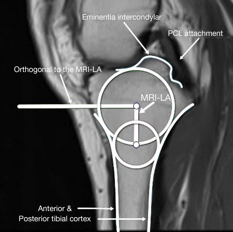
1. Identify the central slice on the MRI where the posterior cruciate ligament (PCL) attaches to the tibia, the intercondylar eminence is visible, and the anterior and posterior tibial cortices are concave.

2. Draw two circles on the tibial head, as shown in Figure 1: a cranial circle and a caudal circle. The cranial circle must touch the anterior, posterior, and cranial tibial cortex bones, while the caudal circle must touch the anterior and posterior cortical borders. The caudal circle should be centered on the perimeter of the cranial circle, and a line connecting their centers serves as the MRI-longitudinal axis (MRI-LA).

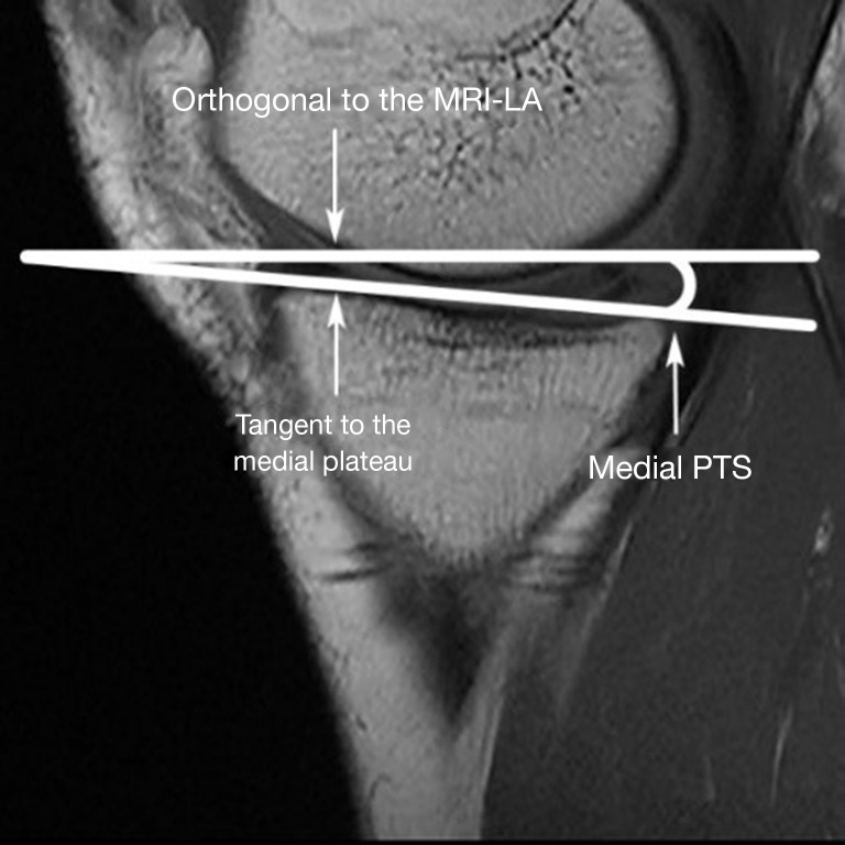
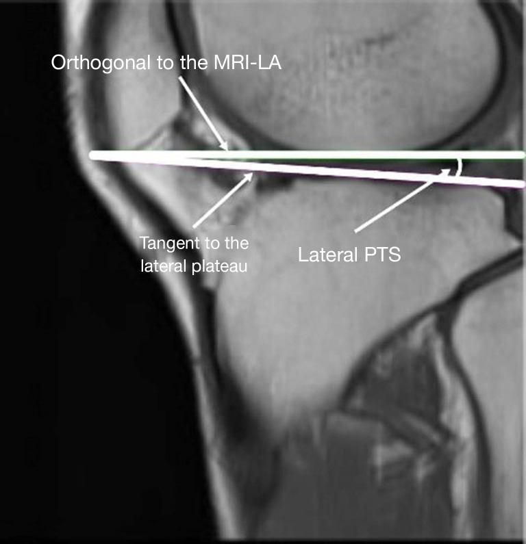
3. Measure the medial and lateral PTS, as illustrated in Figures 2,3, respectively. The medial and lateral PTS are defined as the angle between the tangent to the medial or lateral tibial plateau and the orthogonal to the MRI-LA. The tangent to the medial plateau connects the topmost superior-anterior and posterior cortical edges, while the tangent to the lateral plateau is defined as the uppermost even part of the superior-anterior and posterior cortices.

Figure 1.

The MRI-LA determination on the central slice. MRI-LA, MRI-longitudinal axis; PCL, posterior cruciate ligament; MRI, magnetic resonance imaging.

Figure 2.

Medial PTS measurement. MRI-LA, MRI-longitudinal axis; PTS, posterior tibial slopes; MRI, magnetic resonance imaging.

Figure 3.

Lateral PTS measurement. MRI-LA, MRI-longitudinal axis; PTS, posterior tibial slopes; MRI, magnetic resonance imaging.

Although the PTS measurement method described above is the most reliable and consistent method on MRI (19), its manual measurements used by physicians in practice are often complicated and prone to human error (1). For instance, it takes many iterations for the doctors to ensure that the caudal circle is tangent to the tibial cortical boundary and its center is on the perimeter of the cranial circle, which is not only boring and time-consuming but also has low repeatability. In addition, differences in proficiency and standards among various physicians can introduce errors and ultimately affect the accuracy of determining the MRI-LA and PTS. Comparing with the manual drawing measurement, the development of computer algorithms to implement this measurement technique can be more accurate, efficient, and repeatable (20). Therefore, developing accurate, efficient, and clinically applicable automated methods for measuring PTS is highly demanded.

Hence, this article introduces two new methods for automating the PTS measurement technique. The first approach utilizes traditional image processing algorithms to extract tibia’s contours from the MRI. The second approach employs two deep learning models for image classification and tibia segmentation before the same measurement procedures. These automated techniques can improve the accuracy and efficiency of PTS measurement, benefiting both clinical practice and research. We present this article in accordance with the TRIPOD reporting checklist (available at https://qims.amegroups.com/article/view/10.21037/qims-23-1799/rc).

Methods

This section will discuss the details of the two automatic measurement pipelines and result evaluation approach: the first pipeline using traditional methods will be stated in Section Pipeline 1, while the second pipeline using deep learning models will be discussed in Section Pipeline 2. The study was conducted in accordance with the Declaration of Helsinki (as revised in 2013). The study was approved by the Ethics Committee of the Chinese People’s Armed Police Force General Hospital (the current Third Medical Center of Chinese PLA General Hospital) (approval No. Z181100001718018). Informed consent was taken from all the patients.

Pipeline 1

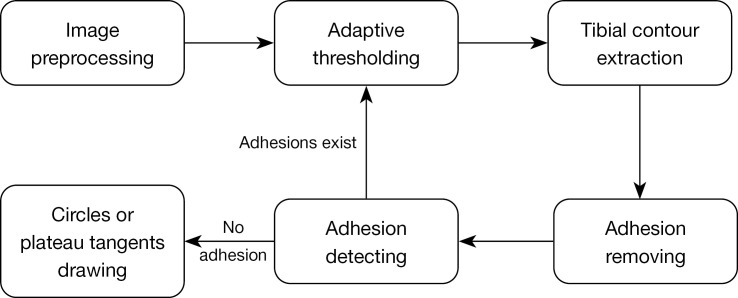
The process of handling the central, medial, and lateral slices in pipeline 1 can be described as a systematic procedure involving several steps, including image preprocessing, adaptive thresholding, extraction of tibial contour, removal of adhesions, detection of adhesions, and finally drawing circles and plateau tangents. The interrelation between these steps is shown in Figure 4. To ensure the quality of the extracted tibial contour, a cyclic process was employed, as shown on the right side of Figure 4.

Figure 4.

The flow chart of pipeline 1.

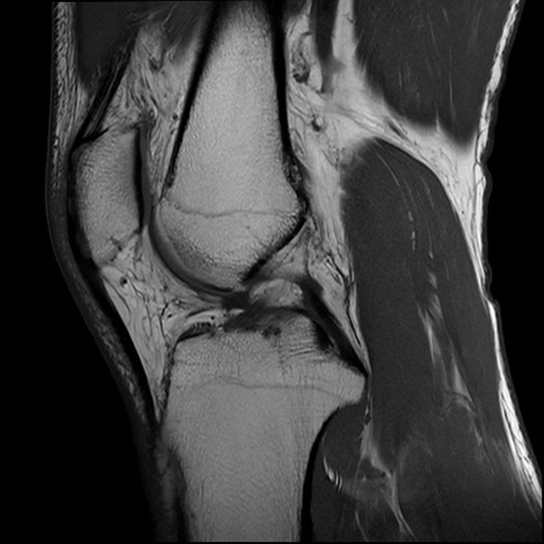
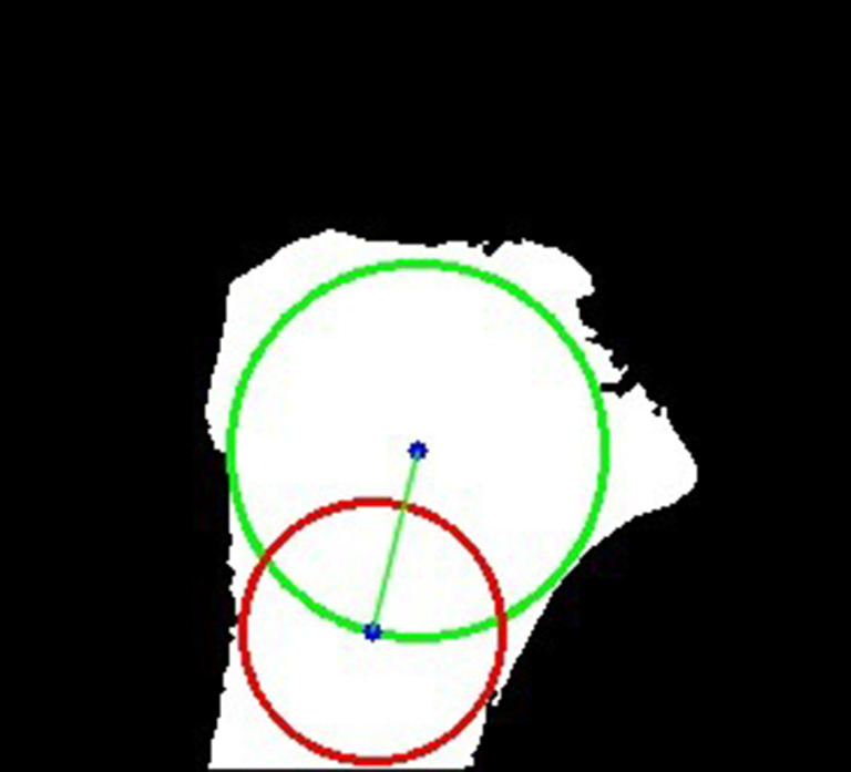
1. Preprocessing. As depicted in the example MRI image Figure 5, the tibial part, which is the only meaningful part for this task, just occupies a very small area on the image. Hence, in order to eliminate the influence of irrelevant regions and facilitate the subsequent tibial contour extraction, the image needs to be pruned. However, the tibial position of different patients varies across their MRI images due to different shooting standards, and imaging positions. Consequently, a broader area should be selected for pruning to ensure complete inclusion of all tibial parts across various patients’ MRI images. The pruning area were determined through experimentation and set to (0.4:1, 0.17:0.73) for images’ height and width.
Additionally, the presence of fissures attached to the tibial edge may affect the radius calculation while drawing circles inside the tibial contour, as illustrated in Figure 6. Therefore, a filter is needed to denoise and smooth the MRI image to reduce fissures after tibia contour extraction. Considering that the denoising methods such as median filtering and Gaussian filtering may blur the edges, leading to deviations in PTS measurements, bilateral filtering, a nonlinear filter that can preserve edge details while denoising, was implemented for this task.

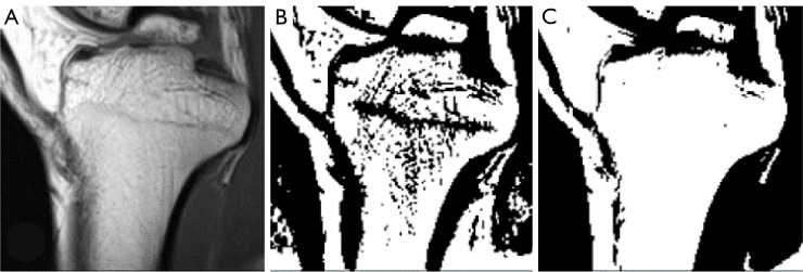
2. Adaptive thresholding. Tibial contour extraction in MRI images was performed after thresholding. Due to the presence of artifacts and adhesions on MRI images, global thresholding techniques which only use one threshold value for the whole image cannot retain the complete tibial edges while trying to segment it perfectly from surrounding tissues, as shown in Figure 7. To overcome this limitation, an adaptive thresholding method from the OpenCV library (21) was employed. This method computes the threshold value for each pixel point by applying global thresholding techniques to a small set of its neighboring pixels at a time. This adaptive approach improves the algorithm’s robustness and enables it to adapt better to the brightness, contrast, and texture of the local area in MRI images.
The determination of the threshold value for each pixel is a critical step that significantly affects the preservation of the tibial contour. The number of neighboring pixels or the size of the pixel neighborhood used to compute the threshold value has a considerable impact on the performance as illustrated in Figure 8. When the number is too large, more neighboring pixels will be considered to determine the local threshold. Hence, the thresholding image will be more comprehensive and the edges will be smoother, but the consequence is the tibial edges may adhere to other tissues, as shown in Figure 8C. On the contrary, if the number of neighboring pixels is too small, the intervals between tibia and surrounding tissues will become more evident, but numerous inwardly recessed cracks may appear inside the tibial contour, which may affect the accuracy of subsequent circle drawing steps, as shown in Figure 8B. Therefore, for MRI images with varying brightness and contrast conditions, this parameter should also be adaptive.

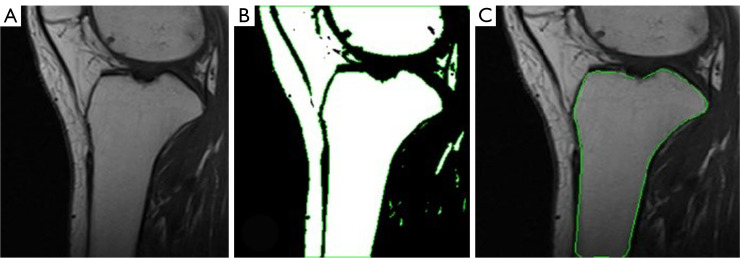
3. Tibial contour extraction. Once a binary image is obtained through adaptive thresholding, the tibial contour extraction process was implemented based on it. The first step was to utilize the OpenCV function findContours (21) to obtain all of the contours on the binary image. Since the tibia is usually the largest area on the processed central slice image, the tibial contour could be determined based on its area size as shown in Figure 9.
However, relying solely on adaptive thresholding may not be sufficient to remove all adhesions completely. In many cases, the tibial contour may not be easily separated from surrounding tissues due to small blurry areas between them, as shown in Figure 8. Continuing to lower this parameter to further segment these small areas may lead to a compromise in contour integrity, which is not desirable. Therefore, after thresholding and contour extraction, it is critical to further remove any remaining adhesions.

4. Adhesion removing. A corner detection algorithm was implemented to identify and remove these adhesions. This procedure includes 4 steps, as illustrated in Figure 10. Firstly, the Harris corner detection algorithm from OpenCV (21) was applied to identify corner points, which are marked in red on Figure 10A. Secondly, the identified corner points were filled in with black to effectively break the adhesions, and the maximum contour was extracted again to obtain the largest boundary as the tibial contour. Thirdly, the corner detection algorithm was run again to search for any recesses created in the second step. Finally, the corner points obtained in step three were marked into white to compensate for the recesses, and a bilateral filtering was performed to smooth the contour.

5. Adhesion detection. Even though several methods for removing adhesions have been applied, it is still important to include an adhesion detection step to ensure that the tibial contour has been accurately segmented.
Due to the large initial value of neighboring pixels, the adhesion removing technique through corner detection may not be effective enough to separate all adhesions. On the contrary, as illustrated in Figure 11, the resulting contour’s area after adhesion removing may even be larger than the input contour due to the fourth step. Hence, the area ratio between resulting contour and input contour was firstly calculated to catch this situation. If the gained ratio exceeds 1.04, it indicates the presence of adhesions and as a result, the value of neighboring pixels parameter should be reduced. This threshold of 1.04 was determined experimentally. Even if the input contour has been a perfect tibial contour before adhesion removing, the resulting contour after adhesion removing could still become slightly larger due to the fourth step, which drew the obtained corner points as white and executed bilateral filtering. Hence, to account for this situation, the threshold was set to 1.04, instead of 1.
Since most of adhesions occur between infrapatellar fat pad (IPFP) and the tibia as shown in Figure 11C, the adhesion detection should focus on this area. Hence, the adhesion detection can be performed by examining if there are white pixels on the upper-left side of the tibia. To this end, the rough position of tibia was obtained firstly to determine the position of its supper left area. As the right side of the tibia do not usually show adhesions, the tibial position search started from determining the tibial rightmost point. Then, on a column of 50 pixels to the left of this point, the first white point from the top to the bottom was detected to determine the position of tibial superior edge. If white pixels are present on a row of 15 pixels above this point, it indicates the presence of this type of adhesion.
Additionally, as shown in Figure 12, there are some adhesions between the tibia and skin that needed to be detected. To address this issue, the convexity defect detection algorithm from OpenCV (21) was utilized. This algorithm identifies “convex defects”, which are the areas that are inside the convex hull of the tibia but outside the contours of the tibia. To detect these defects, the algorithm computes the vertical distance of the convexity defect point to the line connecting the start and end points of the convexity defect. If the calculated distance is at least 30 and the line connecting the start and end points is shorter than 200, then the tibial contour is deemed to contain this type of adhesion. These threshold values were established through experimentation.
Overall, the gain of an eligible tibial contour was a cyclic process as shown in Figure 4. The value of neighboring pixels in the adaptive thresholding algorithm was adjusted based on the quality of the extracted tibial contour after adhesion removal and adhesion detection. Since adhesions attached to the tibial contour are easier to be identified than defects, the adjustment of the value of neighboring pixels in the cyclic process should start from a large value and end with a small value. A large value 251 for this parameter was used as the start. This large value is highly likely to cause adhesion problem. Therefore, after tibial contour extraction and adhesion removing, the aforementioned adhesion detection techniques would be applied to detect if there are any adhesions attaching to the tibial contour. If yes, the number of neighboring pixels would be reduced by a certain amount 20. Thus, in the next iteration, edge adhesions would become less by applying the updated parameter to enhance the boundary separation effect. Then, the adhesion detection was executed again to decide if this parameter should be further reduced to obtain a better tibial edge. This cyclic procedure continues until no adhesions are detected. By using this technique, the tibial contour’s integrity was greatly preserved while reducing adhesions.

6. Circles drawing. After obtaining the final tibial contour, the cranial circle and caudal circle were drawn to determine the MRI-LA. The cranial circle is required to touch the anterior, posterior, and cranial tibial cortex bone, thereby forming the largest circle in the tibial head. In order to determine the center of the cranial circle, the distance from each point within the tibial contour to its nearest contour point was calculated. The point with the greatest distance served as the center of the cranial circle, and this distance was the corresponding radius. The caudal circle is required to touch the anterior and posterior cortical border and its center should be located on the perimeter of the cranial circle. Thus, the distance from each point on the perimeter of the cranial circle to its nearest tibial contour point was computed. The center of the caudal circle was the point with the biggest distance, with the greatest distance serving as its radius. Then, the MRI-LA could be determined by connecting the centers of the circles as shown in Figure 13.

Figure 5.

An example of original MRI image. MRI, magnetic resonance imaging.

Figure 6.

An example of the influence of the fissure to the circle. Green circle: cranial circle. Red circle: caudal circle. Green line: MRI-LA. MRI-LA, MRI-longitudinal axis; MRI, magnetic resonance imaging.

Figure 7.

The global thresholding for two MRI images. (A,C) Example MRI images. (B,D) The resulting images after global thresholding. Green circle: cranial circle. Red circle: caudal circle. Green line: MRI-LA. MRI-LA, MRI-longitudinal axis; MRI, magnetic resonance imaging.

Figure 8.

The adaptive thresholding with different sizes of the pixel neighborhood. (A) The original MRI image. (B) The binary image of 41 pixels neighborhood. (C) The binary image of 141 pixels neighborhood. MRI, magnetic resonance imaging.

Figure 9.

The max contour extraction. (A) Example MRI image. (B) All detected contours on the binary image. (C) The determined tibial contour. MRI, magnetic resonance imaging.

Figure 10.

The 4 steps of adhesion removing. The red areas are detected corner points.

Figure 11.

The example of the contour area becoming bigger after adhesion removing. (A) Example MRI image. (B) Adaptive thresholding result. (C) Tibial contour extraction result. (D) Adhesion removing result. MRI, magnetic resonance imaging.

Figure 12.

Adhesion detection occurring between tibia and skin. (A) Adaptive thresholding result. (B) Adhesion removing result. (C) Tibial contour re-extraction result. (D) Adhesion detection result. The plotted green contour is the detected tibial contour. The red point is a detected convexity defect point. The red line is the connection of the start and end points of the convexity defect.

Figure 13.

An example of tibial bottom extension. (A,B) Circles drawing before extension. (C,D) Circles drawing after extension. Green circle: cranial circle. Red circle: caudal circle. On (A,C), the green line is the MRI-LA. On (B,D), the purple line is the MRI-LA and the green line is its orthogonal. MRI-LA, MRI-longitudinal axis; MRI, magnetic resonance imaging.

Nevertheless, in some cases where the tibia is too short, the caudal circle drawing would be constrained by the tibial bottom, as shown in Figure 13B. This problem can be identified if the distance between the caudal circle’s center and the tibial bottom edge approximately equals its radius. To address this issue, as shown in Figure 13C, the tibial bottom edge would be extended downward by 40 pixels to avoid its interference to the caudal circle drawing.

The medial and lateral slices

On the medial and lateral slices, the tangent to the medial and lateral plateaus would be determined respectively following the process in Figure 4. With the orthogonal to the MRI- LA, the medial and lateral PTS can be measured.

1. Preprocessing. As the tibia areas in the medial and lateral slices become much smaller than in the central slice, and its position is not as fixed as in the central slice, a broad cutting range is necessary when removing irrelevant tissues. Furthermore, to make the cropped image more observable, it was enlarged twice. This resizing operation will not affect the angle measurement as the width and length were scaled by the same factor. In addition, the adaptive thresholding method with predefined parameters would be executed to generate a binary image for contour extraction.

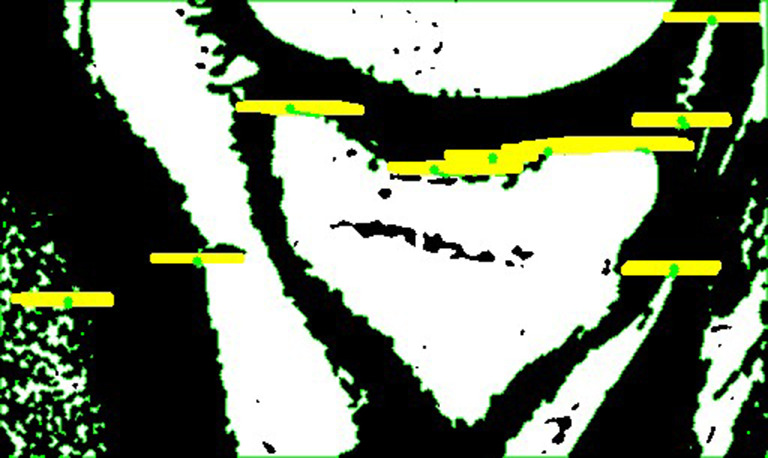
2. Tibial contour extraction. The biggest difference to the central slice is that the tibial area is not the largest area on the medial and lateral slice. Thus, after contour segmentation, the tibial contour cannot be determined directly based its area. A new strategy was proposed to finish this task.
The presence of a black area between the tibia and femur, as shown in Figure 14, indicates a certain distance between them. This pattern can be utilized to identify the tibial contour by counting the number of “concave points” on the contours. A concave point is defined as a contour point above which there is an all-black area of a certain size. The size of the required black area was determined experimentally. The contour with the largest area among the top three contours which had the most concave points would be considered the proposal tibial contour. After this, the adhesion removing and adhesion detection operations would be implemented to remove adhesions and check if the tibial contour without adhesions was extracted successfully. If not, the value of neighboring pixels of the adaptive thresholding algorithm would be adjusted accordingly as aforementioned. The procedures of adaptive thresholding, adhesion removing, and adhesion detection for the medial and lateral slices were similar to those applied in the central slice. The final tibial contour could be obtained following these cyclic operations.

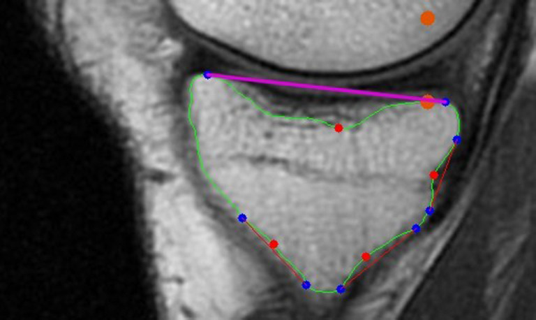
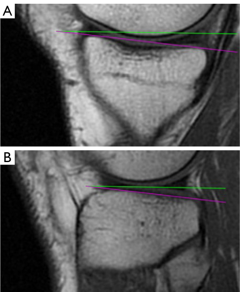
3. The medial and lateral PTS calculation. The convexity defect detection algorithm was implemented on the tibial contour to obtain the start and end points of each convexity defect and the defect points. As shown in Figure 15, the start and end points higher than the point which lower 10 pixels than the tibial rightmost point detected in the adhesion detection section would be considered a pair of proposal points for the tangent of the medial or lateral plateau. The pairs of proposal points with very small distances between them would be filtered out. The remaining pairs of proposal points would be ranked according to their average row values. Then, their slopes would be computed one by one in the order generated before. If the resulting slope rate was not in a reasonable range, the corresponding pair of proposal points would be eliminated. This process would stop while successfully finding the first pair of proposal points with a reasonable slope rate. In conclusion, the highest pair of proposal points with a reasonable slope would be used to draw the tangent of the medial or lateral plateau. Subsequently, the orthogonal to the MRI-LA would be utilized to calculate the medial and lateral PTS as shown in Figure 16.

Figure 14.

The tibial contour determination on the medial slice. The green points are the defined concave points.

Figure 15.

The determination of the tangent of the medial plateau, which is marked in purple. The start and end points of each convexity defect is marked in blue. The defect points are in red. The orange points were used to determine the tangent.

Figure 16.

The measurement of the (A) medial and (B) lateral PTS. The green and purple lines are the orthogonal of MRI-LA and the tangent of medial or lateral plateau. MRI-LA, MRI-longitudinal axis; PTS, posterior tibial slopes; MRI, magnetic resonance imaging.

Pipeline 2

In pipeline 2, two deep learning models, GoogleNet-V2 (22) and U-Net (23), were trained for image classification and tibial contour segmentation. GoogleNet-V2 was used to classify the central, medial, and lateral slices from all the MRI images of a patient. This function was not included in pipeline 1. U-Net was used to segment the tibial contour on the central, medial, and lateral images. This greatly simplifies and improves the corresponding complex cyclic sections in pipeline 1. The remaining PTS measurement sections after slice classification and tibial segmentation are the same as aforementioned in pipeline 1.

Classification

1. Data. The dataset utilized in this study includes a total of 2,261 MRI images in RGB format, obtained from 119 patients. These MRI images were collected from clinical trials of a research project with ethical approval statements in the Third Medical Center of Chinese PLA General Hospital (previous Chinese People’s Armed Police Force General Hospital). Due to the high similarity between adjacent images in each patient’s 19 MRI images, if they are labeled as one central slice, one medial slice, one lateral slice and other 16 irrelevant slices, it would hinder the model’s convergence and overall performance. Therefore, the 2,261 images were labeled by professional physicians as 1,483 irrelevant images, 263 medial images, 194 central images, and 321 lateral images.

2. Preprocessing. To standardize the shapes of the images, all images were resized to 256×256. Since the MRI images are predominantly gray, the RGB images were converted to grayscale. To remove redundant information from the images, they were cropped using a range of (96:256, 30:190). The pixel values in the images were then normalized to a range of (0, 1) to facilitate training of the classification model. The labels for the images were assigned as 0, 1, 2, or 3 to represent useless slices, central slice, medial slice, and lateral slice respectively and they were converted to one-hot vectors for training.

3. Data augmentation. To improve the model’s generalization capability, augmentation techniques such as zoom, horizontal and vertical shift were used during training. The zoom range was (−0.2, 0.2) and the shift range was (0.9, 1.1). Augmentation was applied to the training images with a probability of 50%.

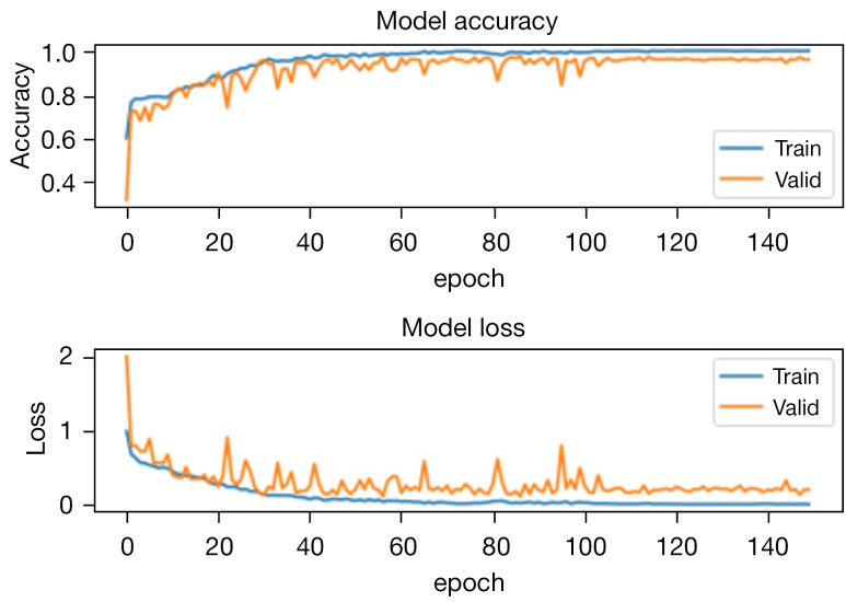
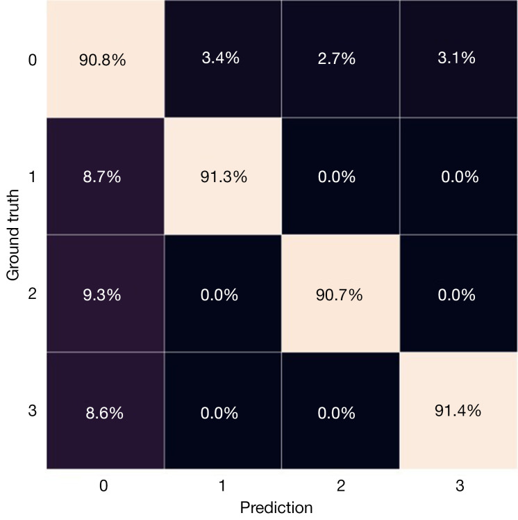
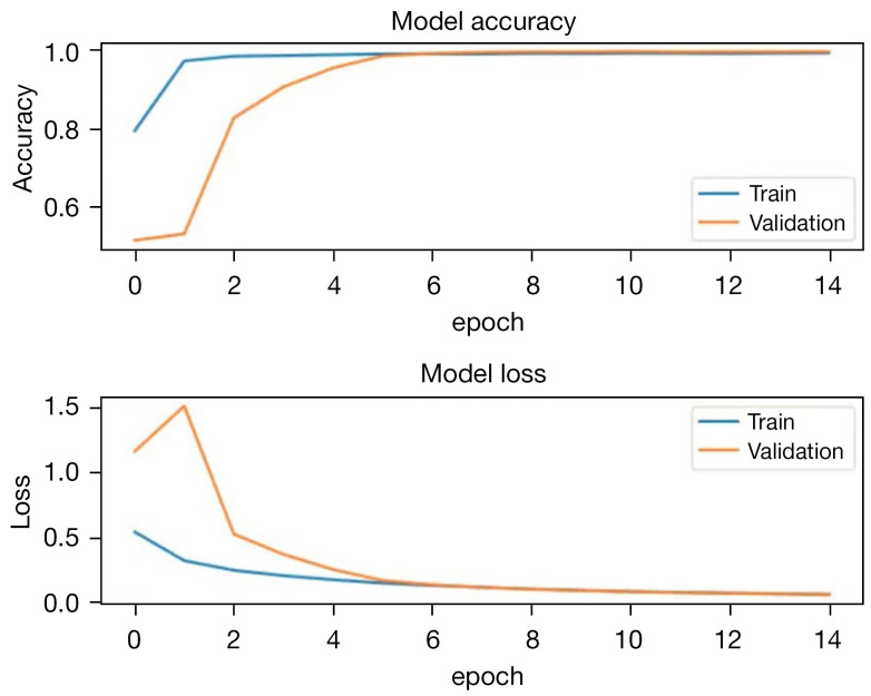
4. Training and testing. The model was trained on a Nvidia GeForce RTX 3060 GPU using Tensorflow and CUDA. The dataset was split into training, validation, and test sets, which comprised 75%, 5%, and 20% of the entire dataset. The batch size for training was set to 80, while for validation, it was 30. RMSprop algorithm was utilized as the optimizer with a learning rate of 0.01. The loss function employed was categorical cross-entropy. The training curves of the model and the confusion matrix of testing are shown in Figures 17,18, respectively.

Figure 17.

The training accuracy and loss curves of classification model.

Figure 18.

The confusion matrix of the trained model on the test set.

Segmentation

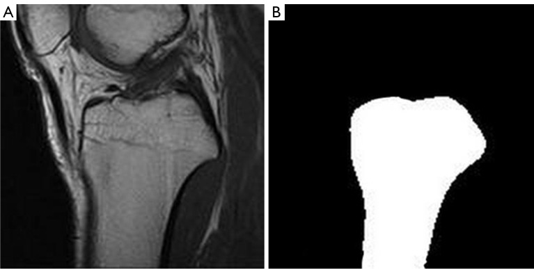
1. Data. The dataset for tibial contour segmentation consisted of 823 MRI images from the aforementioned dataset for classification, along with their corresponding ground truth segmentations generated using our mature pipeline 1. An illustration of a sample image-label pair is shown in Figure 19. The sampled MRI images mainly included central, medial, and lateral MRI slices.

2. Preprocessing. The preprocessing method used in the segmentation section was similar to that in the classification section. The ground truth segmentations were processed using the same techniques to ensure that they still match after preprocessing. Ultimately, the resulting images were grayscale and normalized to 160×160.

3. Data augmentation. Data augmentation was applied during the training process. Five types of transformations were implemented with a probability of 50%, namely rotation, zoom, shift, shear, and horizontal flipping. The ranges of rotation, zoom, shift, and shear were set to (5, 5), (0.9, 1.1), (−0.1, 0.1), and (−0.1, 0.1), respectively. The MRI image and its ground truth were augmented in the same way to ensure they still match after augmentation.

4. Training and testing. A batch size of 180, Adam optimizer with a learning rate of 0.0001 were used for training. Early stopping was employed to prevent overfitting. The loss function was binary cross-entropy. The dataset was divided into training, validation, and test sets, comprising 75%, 5%, and 20% of the entire dataset. The training curves can be observed in Figure 20. The pixel accuracy of the test set was 99.1%.

Figure 19.

An example of training data for segmentation model. (A) MRI image. (B) Ground truth segmentations. MRI, magnetic resonance imaging.

Figure 20.

The training accuracy and loss curves of segmentation model.

Result evaluation

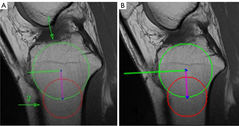
Each pipeline was integrated into a software tool for evaluators to validate and compare their practical performance and effectiveness. The evaluation of images from the software was independently conducted by two evaluators. One was an orthopedic attending physician with professional experience in this area, the other one was an internship student who was previously unfamiliar with this measurement technique. A total of 380 MRI images from 20 patients were utilized in the evaluation. For each patient, the central, medial, and lateral slice images were manually selected by the doctors and fed into both pipelines for PTS measurements. To validate the accuracy and effectiveness of the obtained medial and lateral PTS, evaluators focused on the positions of the cranial and caudal circles, as well as the tangents to the medial and lateral plateaus. Specifically, to verify the accuracy of the obtained MRI-LA on the central slice, evaluators observed whether the anterior, posterior, and cranial tibial cortex bones touched the cranial circle, and whether the anterior and posterior cortical borders touched the caudal circle. For the medial and lateral slices, evaluators checked the accuracy of the obtained tangents. Furthermore, evaluators compared the results from two pipelines and determined which one works better. The focus primarily lay on discerning differences in the extracted tibial contours, particularly in locations that may impact subsequent circle drawing and tangent determination. A pair of examples are shown in Figure 21 to illustrate this assessment approach. Figure 21A is the resulting image from pipeline 1, while Figure 21B presents the result of pipeline 2. Although the resulting images from both pipelines are successful and the angles of the obtained MRI-LA axes differed by only 0.1 degrees, pipeline 2 performs better comparing the circles drawn in the areas indicated by arrows 1 and 2. Upon careful observation of these two areas, it can be found that the tibial edges are relatively ambiguous there. The region pointed by arrow 1 seems to be where the tibia adheres to the tissue above it, with no clear tibial edge apparent. Similarly, the tibial cortex in the region indicated by arrow 2 is also relatively indistinct on MRI. The indistinct boundaries of these two critical areas presents considerable obstacles to the tibial contour extraction algorithm of pipeline 1, thereby affecting the subsequent drawing of circles.

Figure 21.

An example of the evaluation approach. (A) Pipeline 1. (B) Pipeline 2. Green circle: cranial circle. Red circle: caudal circle. Purple line: MRI-LA. Green line: the orthogonal of MRI-LA. MRI-LA, MRI-longitudinal axis; MRI, magnetic resonance imaging.

Results

The summary of the evaluation experiment is presented in Table 1 and the comparison between two pipelines is shown in Table 2. Regarding the assessment of success and failure, both evaluators reached the same conclusions, as visually confirming whether the automated pipelines accurately drew the circles and tangents was not particularly challenging. However, when it comes to results comparison of two pipelines, there were a few of small differences between their evaluation results. Given the orthopedic attending physician is more professional, we took his evaluation result as the final result used in Table 2.

Table 1. The success and failure numbers of both pipelines in terms of central, medial, and lateral slices in the evaluation experiment.

Slice	Pipeline 1			Pipeline 2
	Failure	Success		Failure	Success
Central	3	17 (85%)		0	20 (100%)
Medial	0	20 (100%)		0	20 (100%)
Lateral	2	18 (90%)		1	19 (95%)

Table 2. The comparison of two pipelines on each MRI slice.

Slice	Pipeline 1 better	Pipeline 2 better	Deuce
Central	1	4	15
Medial	5	8	7
Lateral	4	12	4

MRI, magnetic resonance imaging.

Discussion

The automated pipelines for PTS measurement proposed in this study are characterized by high efficiency and robustness. They are able to measure both medial and lateral PTS from MRI slices. Compared to manual measurements performed by experienced physicians using mapping software, which typically take about 10 minutes per patient, the proposed pipelines require only about 10 seconds. Moreover, according to Hudek et al. (2009), the interobserver and intraobserver reproducibility of this circle method were 0.77 and 0.80 respectively assessed using intraclass correlation coefficient (ICC). This slightly lower reproducibility on MRI comes from the fact that several images are assessed in consecutive steps, instead of only one image is used for lateral radiograph (16). The discrepancies might arise from some minor differences in plotting standard, human error, or some factors that are difficult to standardize throughout the manual measurement process. Our automated pipelines could be a solid foundation for mitigating these deviations and enhancing the reliability and reproducibility of results. This is particularly advantageous for large-scale studies or those involving numerous doctors investigating the role of PTS in ACL and other clinical researches related to knee biomechanics. In addition, our automated pipelines enrich the application of deep learning in clinical procedures.

While the process of training the classification model is arduous, its practical significance is limited as physicians can rapidly identify the required slices. For the extraction of tibial contours, although the traditional image processing methods can solve this problem well, due to the complex nature of MRI images, it is inevitable to pay the price of an increase in the algorithmic complexity as well as a decrease in its adaptability to deal with the details that may exist on some few images in a targeted manner. Furthermore, there are significant differences between the processing of specific details in the central and medial, lateral layers. Consequently, traditional image processing methods would require separate extraction algorithms to be designed for each layer’s distinct characteristics. In contrast, deep learning-based segmentation model enables the use of a single model to extract tibial contours across three different slices, substantially reducing workload.

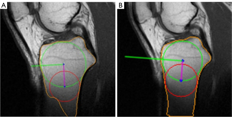
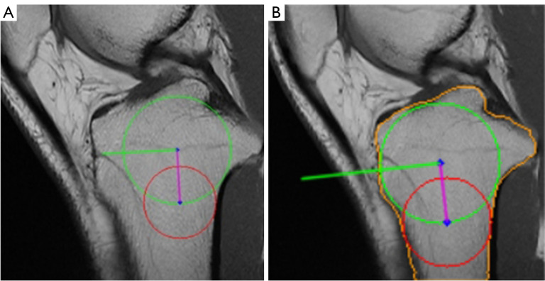
Upon evaluating the results, it is evident that pipeline 2 outperforms pipeline 1 in terms of a higher success rate and better outcome. The only instance of failure in pipeline 2 on the lateral slice occurred due to the prominent lateral tibial plateau. The superiority of pipeline 2 is attributed to the segmentation model’s ability to directly extract a more precise tibial contour. Although the traditional tibial contour extraction method can successfully extract most contours, it occasionally faces issues such as concave tibial edges, which can affect subsequent measurements due to the automatic adjustment of parameters. The cyclic process of tibial contour extraction is complex, and the parameters of the applied algorithms are set experimentally, which impairs the robustness of pipeline 1. As shown in Figures 22,23, pipeline 1 is unable to extract the precise tibial contour due to its inherent limitations. In contrast, the deep learning model in pipeline 2 can adjust to the impact of luminance and cracks. Moreover, pipeline 2 demonstrates considerably better results than pipeline 1, particularly in the lateral slice. This can be attributed to the potential defocusing of the boundary at the anterior and posterior ends of the tibia, which can marginally impact lateral PTS measurement.

Figure 22.

Pipeline 1 failed because of the blurry tibial bottom. (A) Pipeline 1. (B) Pipeline 2. Green circle: cranial circle. Red circle: caudal circle. Purple line: MRI-LA. Green line: the orthogonal of MRI-LA. The detected tibial contour is marked in orange. MRI-LA, MRI-longitudinal axis; MRI, magnetic resonance imaging.

Figure 23.

Pipeline 1 failed due to the crack inside the tibia. (A) Pipeline 1. (B) Pipeline 2. Green circle: cranial circle. Red circle: caudal circle. Purple line: MRI-LA. Green line: the orthogonal of MRI-LA. The detected tibial contour is marked in orange. MRI-LA, MRI-longitudinal axis; MRI, magnetic resonance imaging.

Despite the significant simplification of the entire process through the use of deep learning models, the demand for a large number of well-annotated masks for model training is costly. However, fortunately, pipeline 1 is a white box and can be a valuable tool for generating the required ground truth segmentations for training the black-box deep learning model.

The deep learning models employed in this study are not the latest models for classification and segmentation. To further improve efficiency and accuracy, we will explore more effective models and novel techniques in the future. Moreover, we are planning to add an extra function to the current software. It will enable manual adjustments by humans to the location, radius, and angles of the plotted circles and tangents generated by the automated pipelines. With this function, even if the results from the pipelines are not as reliable as those from human assessment, they can still serve as a basis for further refinement by humans. This approach can guarantee the measurement accuracy while speeding up the measurement process. In addition, considering the presence of hardware in the knees of ACL-reconstructed patients, which has the potential to amplify artifacts or impact the outcomes of PTS measurements on MRI, it could be better if the future automated pipelines are able to adapt to this scenario.

Conclusions

This paper proposes two accurate, efficient, automatic measurement pipelines of the circle method to measure the medial and lateral PTS on MRI images. A software incorporating these two pipelines are designed to aid doctors during clinical decision making. It enables doctors to use the circle method to measure PTS within 10 seconds, providing a remarkable speed improvement of nearly 60 times compared to the 10 minutes required for manual measurement. Using these automated pipelines can also reduce human errors, enhance measurement accuracy, and improve clinical result repeatability, which is crucial for reusing and comparing measurements in different PTS researches. As the first automated tool for the most repeatable measurement techniques proposed by Hudek et al. (2009), it has the potential to facilitate the study of the significance of PTS for ACL injury and its reconstruction surgeries, the comparison of different measurement methods, and even the development of new ones.

Supplementary

The article’s supplementary files as

Ethical Statement: The authors are accountable for all aspects of the work in ensuring that questions related to the accuracy or integrity of any part of the work are appropriately investigated and resolved. The study was conducted in accordance with the Declaration of Helsinki (as revised in 2013). The study was approved by the Ethics Committee of the Chinese People’s Armed Police Force General Hospital (the current Third Medical Center of Chinese PLA General Hospital) (approval No. Z181100001718018). Informed consent was taken from all the patients.

References

- 1.Domnick C, Raschke MJ, Herbort M. Biomechanics of the anterior cruciate ligament: Physiology, rupture and reconstruction techniques. World J Orthop 2016;7:82-93. 10.5312/wjo.v7.i2.82 [DOI] [PMC free article] [PubMed] [Google Scholar]
- 2.He M, Li J. Increased lateral femoral condyle ratio measured by MRI is associated with higher risk of noncontact anterior cruciate ligament injury. BMC Musculoskelet Disord 2022;23:190. 10.1186/s12891-022-05134-x [DOI] [PMC free article] [PubMed] [Google Scholar]
- 3.Zhang ZY, Pan XY, Maimaitijiang P, Meng LY, He ZY, Zhao Q, Wang C, Wang JQ. Anterior tibial subluxation measured under a modified protocol is positively correlated with posterior tibial slope: a comparative study of MRI measurement methods. Knee Surg Sports Traumatol Arthrosc 2022;30:3350-60. 10.1007/s00167-022-06913-8 [DOI] [PubMed] [Google Scholar]
- 4.Wong CK, Man GCW, He X, Ng JP, Ng AWH, Ong MTY, Yung PSH. Large lateral tibial slope and lateral-to-medial slope difference are risk factors for poorer clinical outcomes after posterolateral meniscus root tear repair in anterior cruciate ligament reconstruction. BMC Musculoskelet Disord 2022;23:247. 10.1186/s12891-022-05174-3 [DOI] [PMC free article] [PubMed] [Google Scholar]
- 5.Beaulieu ML, Ashton-Miller JA, Wojtys EM. Loading mechanisms of the anterior cruciate ligament. Sports Biomech 2023;22:1-29. 10.1080/14763141.2021.1916578 [DOI] [PMC free article] [PubMed] [Google Scholar]
- 6.Beynnon BD, Hall JS, Sturnick DR, Desarno MJ, Gardner-Morse M, Tourville TW, Smith HC, Slauterbeck JR, Shultz SJ, Johnson RJ, Vacek PM. Increased slope of the lateral tibial plateau subchondral bone is associated with greater risk of noncontact ACL injury in females but not in males: a prospective cohort study with a nested, matched case-control analysis. Am J Sports Med 2014;42:1039-48. 10.1177/0363546514523721 [DOI] [PMC free article] [PubMed] [Google Scholar]
- 7.Pearce SL, Bryniarski AR, Brown JR, Brady AW, Gruskay JA, Dornan GJ, Vidal AF, Godin JA. Biomechanical Analysis of Tibial Motion and ACL Graft Forces After ACLR With and Without LET at Varying Tibial Slopes. Am J Sports Med 2023;51:2583-8. 10.1177/03635465231184389 [DOI] [PubMed] [Google Scholar]
- 8.Yoshihara A, Siboni R, Nakagawa Y, Mouton C, Jacquet C, Nakamura T, Sekiya I, Seil R, Koga H. Lateral-medial asymmetry of posterior tibial slope and small lateral tibial plateau articular surface depth are morphological factors of lateral meniscus posterior root tears in ACL-injured patients. Knee Surg Sports Traumatol Arthrosc 2023;31:3594-603. 10.1007/s00167-023-07317-y [DOI] [PubMed] [Google Scholar]
- 9.Edwards TC, Naqvi AZ, Dela Cruz N, Gupte CM. Predictors of Pediatric Anterior Cruciate Ligament Injury: The Influence of Steep Lateral Posterior Tibial Slope and Its Relationship to the Lateral Meniscus. Arthroscopy 2021;37:1599-609. 10.1016/j.arthro.2020.12.235 [DOI] [PubMed] [Google Scholar]
- 10.Fares A, Horteur C, Abou Al Ezz M, Hardy A, Rubens-Duval B, Karam K, Gaulin B, Pailhe R. Posterior tibial slope (PTS) ≥ 10 degrees is a risk factor for further anterior cruciate ligament (ACL) injury; BMI is not. Eur J Orthop Surg Traumatol 2023;33:2091-9. 10.1007/s00590-022-03406-9 [DOI] [PMC free article] [PubMed] [Google Scholar]
- 11.Guo N, Smith CR, Schütz P, Trepczynski A, Moewis P, Damm P, Maas A, Grupp TM, Taylor WR, Hosseini Nasab SH. Posterior tibial slope influences joint mechanics and soft tissue loading after total knee arthroplasty. Front Bioeng Biotechnol 2024;12:1352794. 10.3389/fbioe.2024.1352794 [DOI] [PMC free article] [PubMed] [Google Scholar]
- 12.Tanaka T, Gale T, Nishida K, Xu C, Fu F, Anderst W. Posterior tibial slope and meniscal slope correlate with in vivo tibial internal rotation during running and drop jump. Knee Surg Sports Traumatol Arthrosc 2023;31:2366-73. 10.1007/s00167-022-07163-4 [DOI] [PubMed] [Google Scholar]
- 13.Ahmed I, Salmon L, Roe J, Pinczewski L. The long-term clinical and radiological outcomes in patients who suffer recurrent injuries to the anterior cruciate ligament after reconstruction. Bone Joint J 2017;99-B:337-43. 10.1302/0301-620X.99B3.37863 [DOI] [PubMed] [Google Scholar]
- 14.Hashemi J, Chandrashekar N, Mansouri H, Gill B, Slauterbeck JR, Schutt RC, Jr, Dabezies E, Beynnon BD. Shallow medial tibial plateau and steep medial and lateral tibial slopes: new risk factors for anterior cruciate ligament injuries. Am J Sports Med 2010;38:54-62. 10.1177/0363546509349055 [DOI] [PubMed] [Google Scholar]
- 15.Ye Z, Xu J, Chen J, Qiao Y, Wu C, Xie G, Dong S, Zhao J. Steep lateral tibial slope measured on magnetic resonance imaging is the best radiological predictor of anterior cruciate ligament reconstruction failure. Knee Surg Sports Traumatol Arthrosc 2022;30:3377-85. 10.1007/s00167-022-06923-6 [DOI] [PubMed] [Google Scholar]
- 16.Hudek R, Schmutz S, Regenfelder F, Fuchs B, Koch PP. Novel measurement technique of the tibial slope on conventional MRI. Clin Orthop Relat Res 2009;467:2066-72. 10.1007/s11999-009-0711-3 [DOI] [PMC free article] [PubMed] [Google Scholar]
- 17.Vieider RP, Mehl J, Rab P, Brunner M, Schulz P, Rupp MC, Siebenlist S, Hinz M. Malrotated lateral knee radiographs do not allow for a proper assessment of medial or lateral posterior tibial slope. Knee Surg Sports Traumatol Arthrosc 2024;32:1462-9. 10.1002/ksa.12170 [DOI] [PubMed] [Google Scholar]
- 18.Sauer S, Clatworthy M. Editorial Commentary: The Ratio of Tibial Slope and Meniscal Bone Angle is a Strong Predictor for Anterior Cruciate Ligament Injury: A Steep Hill and a Shallow Speed Bump are a Hazardous Combination. Arthroscopy 2021;37:1610-1. 10.1016/j.arthro.2021.02.006 [DOI] [PubMed] [Google Scholar]
- 19.Lipps DB, Wilson AM, Ashton-Miller JA, Wojtys EM. Evaluation of different methods for measuring lateral tibial slope using magnetic resonance imaging. Am J Sports Med 2012;40:2731-6. 10.1177/0363546512461749 [DOI] [PMC free article] [PubMed] [Google Scholar]
- 20.Akhavi Milani A, Motallebzadeh Khanamiri M, Mahmoudpour M. The geometric features of tibiofemoral joint associated with anterior cruciate ligament injury: Reliability of measurements on conventional MRI. Eur J Radiol Open 2022;9:100420. 10.1016/j.ejro.2022.100420 [DOI] [PMC free article] [PubMed] [Google Scholar]
- 21.Bradski G. The OpenCV Library. Dr Dobb’s Journal of Software Tools 2000;120:122-5. [Google Scholar]
- 22.Ioffe S, Szegedy C, editors. Batch normalization: Accelerating deep network training by reducing internal covariate shift. Proceedings of the 32nd International Conference on Machine Learning, PMLR 2015;37:448-56. [Google Scholar]
- 23.Ronneberger O, Fischer P, Brox T. U-Net: Convolutional Networks for Biomedical Image Segmentation. In: Navab N, Hornegger J, Wells W, Frangi A. editors. Medical Image Computing and Computer-Assisted Intervention – MICCAI 2015. Lecture Notes in Computer Science, Springer, 2015;9351:234-41. [Google Scholar]
Associated Data
This section collects any data citations, data availability statements, or supplementary materials included in this article.
Supplementary Materials