A Representation Theory Perspective on Simultaneous Alignment and Classification

Abstract

Single particle cryo-electron microscopy (EM) is a method for determining the 3-D structure of macromolecules from many noisy 2-D projection images of individual macromolecules whose orientations and positions are random and unknown. The problem of orientation assignment for the images motivated work on general multireference alignment. The recently introduced non-unique games framework provides a representation theoretic approach to alignment over compact groups, and offers a convex relaxation which is formulated as semidefinite programs with certificates of global optimality under certain circumstances. One of the great opportunities in cryo-EM is studying heterogeneous samples, containing two or more distinct classes or conformations of molecules. Taking advantage of this opportunity presents an algorithmic challenge: determining both the class and orientation of each particle. We generalize multireference alignment to a problem of alignment and classification, and we propose to extend non-unique games to the problem of simultaneous alignment and classification with the goal of simultaneously classifying cryo-EM images and aligning them within their respective classes.

1. Introduction

A Non-Unique Game (NUG) is an optimization problem or a statistical estimation problem, of inferring $n$ elements of a group $g_1,\dots ,g_n\in 𝒢$ by minimizing an expression of the form

$$\underset{g_1,\dots ,g_n\in 𝒢}{\text{arg}\text{min}}\sum _{i,j=1}^n{f}_{ij}\left(g_i{g}_j^{-1}\right),$$ (1)

where $f_{ij}:𝒢\to \mathbb{R}$ are loss functions for particular pairwise relations $g_i{g}_j^{-1}$ between elements. This problem arises in multireference alignment (MRA) discussed in [1], and in more general settings discussed in [2]; A convex relaxation of the problem, proposed in [2], can be solved using semidefinite programming (SDP). NUG over the group ${\mathbb{Z}}_2$ and its SDP relaxation coincides with classification problems and graph-cut algorithms (e.g., [3, 4]).

One of the applications where NUGs and associated algorithms have been of particular interest is single particle cryo-electron microscopy (cryo-EM) [5, 6], where multiple noisy 2-D projections images of individual, ideally identical, frozen-hydrated 3-D macromolecules whose orientations and positions are random and unknown, must be aligned over SO(3), as a step in reconstructing the macromolecule. Some of the popular software used for analysis of cryo-EM data (e.g. [7]) alternate between updating an estimate of the scattering density of the molecule and updating an estimate of particle orientations, and are sensitive to scattering density chosen for initialization. One approach to ab-initio modeling of molecules from cryo-EM data, discussed in further detail in Section 2.1 and in [8, 9, 10, 11], uses common lines in the Fourier transforms of particle images to align them. The Fourier transform of these 2-D particle images are slices of the 3-D Fourier transform of the scattering density of the molecule, therefore each two slices have a common line where they intersect. This approach to ab-initio modeling has been formulated as a NUG [2], with the potential advantage of certificates of global optimality and no need for an approximate structure for initialization; the software is under development at the time of writing this paper. Such ab-initio models are used to initialize other algorithms, and to recover smaller structures.

Cryo-EM has been the subject of the 2017 Nobel Prize in Chemistry, due to the breakthroughs that the method facilitated in mapping the structure of molecules that are difficult to crystallize. Cryo-EM does not require crystallization necessary for X-ray crystallography, and unlike NMR it is not limited to small size molecules. One of the additional great opportunities in cryo-EM, is to overcome heterogeneity in the sample [12]: in practice many samples contain two (or more) distinct types of molecules (or different conformations of the same molecule); methods like X-ray crystallography and NMR, which measure ensembles of particles, have a difficulty distinguishing between these different types. In the case of heterogeneous samples, we do not know the orientation or the conformation of the molecule in each particle image; it is therefore natural to ask how MRA can be accomplished before classification of the particle images, or how classification can be accomplished before the particle images are aligned.

In this paper we discuss the problem of alignment and classification, referred to as heterogeneous MRA, and propose to solve them simultaneously. This approach is based on the observation that both alignment and classification are problems over compact groups, and that the direct product of these groups is also a compact group.

We reformulate the problem as an optimization problem over the direct product of the groups, and reduce it to a NUG. In addition, we discuss some of the symmetries in the problem, which are exploited to reduce the size of the resulting SDPs. Furthermore, we propose an approach for controlling the size of the classes. The approach can be generalized to simultaneous alignment and parametrization, in the case of continuous heterogeneity (which will be discussed in a future paper). We demonstrate the applicability of this approach with examples of simoultanous alignment and classifcation over SO(2), comparing the quality of classification to a method of alignment-free classification based on invariant features.

Our approach is also applicable to other recently proposed methods of optimization over groups (e.g. [13, 14, 15]). The idea introduced in this work to treat alignment and classification/heterogeneity as two sides of the same coin in MRA has since been generalized to algorithms that take other perspectives on MRA and heterogeneity (inter alia [16, 17, 18, 19]).

This work suggests that the NUG solver for cryo-EM (developed for the homogeneous case) can be extended to solve the alignment and classification problems simultaneously in the case of heterogeneous cryo-EM samples; the algorithm inherits the properties of the NUG solver, such as certificates of global optimality in some cases and not requiring an approximate structure for initialization. Analogously to the role of ab-initio modeling in the homogeneous case, we envision this type of algorithms used in ab-initio modeling of heterogeneous samples, providing multiple 3-D structures or classification and alignment as initialization for refinement algorithms.

This paper is organized as follows. In Sections 2.1 and 2.2 we present a brief overview of cryo-EM as motivation for the discussion of simultaneous alignment and classification. The remainder of Section 2 summarizes some standard results used in this paper, as well as some previous work on NUGs. Section 3 contains a more detailed discussion of the problem, and the derivation of the main arguments in this paper. In section 4 we propose SDP algorithms for simultaneous alignment and classification. Section 5 contains experimental results for the case of simultaneous alignment and classification over SO(2). In section 6 we summarize our conclusions and briefly discuss generalizations and future work.

2. Preliminaries

2.1. The Cryo-EM Problem

Electron microscopy is an important tool for recovering the 3-D structure of molecules. Of particular interest in the context of this paper is single particle reconstruction (SPR), and more specifically, cryo-EM, where multiple noisy 2-D projections, ideally of identical particles in different orientations, are used in order to recover the 3-D structure. The following formula is a simplified imaging model of SPR

$$\left({𝒫}_R𝒳\right)(x,y)={\int }_z𝒳\left(Rr\right)dz$$ (2)

where $r=(x,y,z)$, $R$ is some random rotation matrix in SO(3), $𝒳$ is the scattering density of the molecule, and $𝒫$ is the projection operator. In other words, the model is that the molecule is rotated in a random direction, and the image obtained is the top-view projection of the rotated molecule, integrating out the $z$ axis. Indeed, one of the characteristic properties of cryo-EM SPR that sets it apart from other tomography techniques is that the orientation $R$ of the molecule in each image is unknown in cryo-EM, whereas in other tomography techniques the rotation angles are typically recorded with the measurements. The analysis of cryo-EM images is further complicated by extremely high level of noise, far exceeding the signal in magnitude, which makes it difficult not only to analyze the particles in the images, but also to locate the particles in the micrographs produced. Sample images are presented in fig. 1. More detailed discussions of these challenges, and various other challenges, such as the contrast transfer functions (CTF) applied to the images in the imaging process, can be found, for example, in [5].

Figure 1:

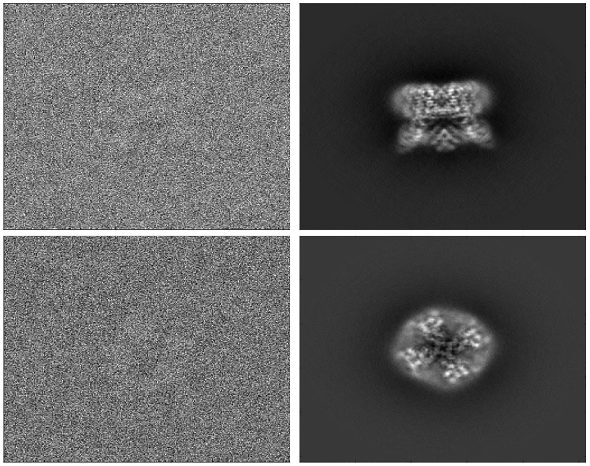
Left: two raw experimental images of TRPV1, available via EMDB 5778 [21]. Right: computed projections of TRPV1 which are the closest to the images on their left.

The reconstruction of the molecule (or, more precisely, the density $𝒳$) from the images obtained in cryo-EM requires an estimate of the rotation angles of the images. The Fourier slice theorem (see, for example, [20]) provides a way to estimate these rotations from the common lines between the images (see, for example [8, 9, 10, 11], and fig. 2). In the context of this paper, we assume that for every pair of images $i$ and $j$, we have some function $f_{ij}\left(g\right)$ which corresponds to the “incompatibility” between the images $i$ and $j$ for every relative orientation $g\in SO\left(3\right)$; this function is a measure of the discrepancy between the radial line in the Fourier transform of image $i$ and the radial line in the Fourier transform of image $j$ which would have corresponded to the common line between the plane of $i$ and the plane of $j$, if the relative orientation of the two images had been $g$. Had there not been noise, we would have expected that $f_{ij}\left(g_{ij}\right)=0$ for the true relative rotation $g_{ij}$ between image $i$ and image $j$, and $f_{ij}\left(g\right)>0$ for every other $g$ (in fact, $f_{ij}\left({\tilde{g}}_{ij}\right)=0$ for every ${\tilde{g}}_{ij}$ that yields the same common lines for the pair of images as $g_{ij}$ since various rotations can yield the same common line. The ambiguity is resolved, up to reflections, only by adding a third image). In practice, due to the high levels of noise, $f_{ij}$ need not be 0 at $g_{ij}$, and in fact, the value of $f_{ij}$ may even not be minimized at $g_{ij}$. However, the expected value of $f_{ij}$ is lower for the true $g_{ij}$ than it is for other relative rotations. For more details about this loss function in the context of this paper, see [2].

Figure 2:

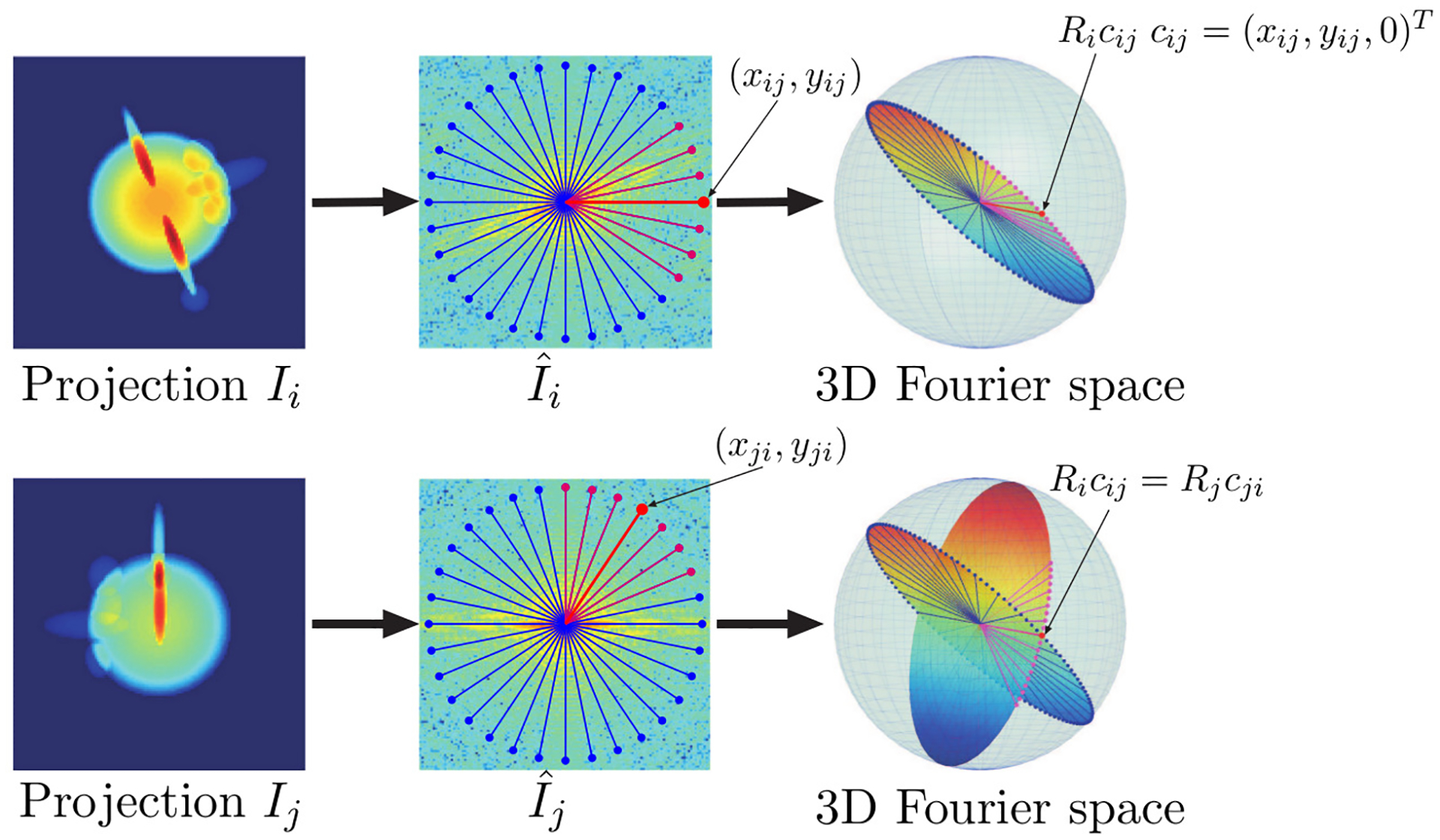
Common Lines in cryo-EM. The left most images $I_i$ and $I_j$ are examples of projections of a molecule density $𝒳$; each projection is obtained from a different direction. At the center, are the Fourier transforms ${\hat{I}}_i$ and ${\hat{I}}_j$ of those images, overlaid with radial lines. The lower right sub-figure is a visualization of the two slices of the 3-D Fourier transform of the 3-D density $𝒳$, corresponding to ${\hat{I}}_i$ and ${\hat{I}}_j$; the two slices intersect each other, so that there is a line in ${\hat{I}}_i$ that is identical to a line in ${\hat{I}}_j$ (assuming no noise). Indeed, the point $\left(x_{ij},y_{ij}\right)$ which lies along this common line in ${\hat{I}}_i$ is identical to the point $\left(x_{ji},y_{ji}\right)$ which lies along this common line in ${\hat{I}}_j$. A more detailed discussion of common lines is available, for example, in [8, 9, 10, 11]

2.2. The Heterogeneity Problem in Cryo-EM

So far, we have assumed that all the molecules being imaged in an experiment are identical copies of each other, so that all the images are projections of identical copies, from different directions. However, in practice, the molecules in a given sample may differ from one another for various reasons. For example, the sample may contain several types of different molecules due to some contamination or feature of the experiment. Alternatively, the molecules which are studied may have several different conformations or states, or some local variability (see example in fig. 3). The heterogeneity may be discrete (e.g. in the case of distinct different molecules) or continuous (in the case of molecules with continuous variability).

Figure 3:

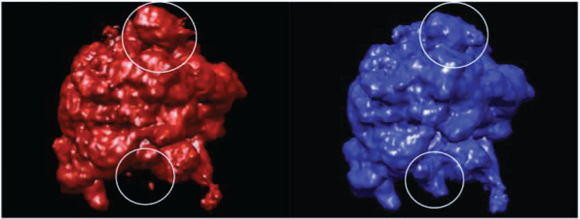
Classical (left) and hybrid (right) states of 70S E. Coli ribosome (image source: [27]).

When there is heterogeneity in the samples, high resolution reconstruction of the molecules requires not only an estimate of the rotation of each image, but also classification of the images into clusters, each corresponding to a different molecule which is to be reconstructed separately. Some of the existing SPR analysis methods rely on some prior knowledge of the underlying molecules and on iterative processes of estimating the structure of the molecules and matching images to those estimates (e.g. [22, 23, 7]), and others require some method of recovering the rotation of the images although the images reflect mixtures of projections of different molecules (e.g. [24, 25]). A recent independent work [26] proposes to iterate between estimating the orientations and estimating the class labels based on pairwise relations between images.

2.3. Irreducible Representations of Groups

The purpose of sections 2.3 to 2.5 is to briefly review some standard results in group theory and harmonic analysis; more detailed discussions of these facts can be found, inter alia, in [28, 29, 30].

Suppose that $𝒢$ is a compact group and $f\in L^2\left(𝒢\right)$, then by the Peter-Weyl Theorem [31], the generalized Fourier expansion of $f$ is

$$f\left(g\right)=\sum _k{d}_k\mathit{\text{tr}}\left({\hat{f}}^{\left(k\right)}{\rho }_k\left(g\right)\right),$$ (3)

where the matrices ${\rho }_k\left(g\right)$ are the irreducible representations of $𝒢,d_k$ is the dimensionality of the $k$th representation, and the matrices ${\hat{f}}^{\left(k\right)}$ are the Fourier coefficients of $f$, defined by the formula

$${\hat{f}}^{\left(k\right)}=\underset{𝒢}{\int }f\left(g\right){\rho }_k^{\text{*}}\left(g\right)dg,$$ (4)

with $dg$ the Haar measure on $𝒢$ normalized so that

$${\int }_{𝒢}dg=1.$$ (5)

Remark 1. For abelian groups, such as SO(2) (shifts on a circle), $d_k=1$ for all k. However, in SO(3), which is of particular interest in the cryo-EM application, $d_k=2k+1$ with $k=\mathrm{0,1},2,\dots$.

The integration of any irreducible representation with respect to the Haar measure yields the zero matrix, except for the case of the trivial constant irreducible representation ${\rho }_0$:

$${\int }_{𝒢}{\rho }_k\left(g\right)dg=0\hspace{1em}\forall k\ne 0.$$ (6)

The following are well known properties of irreducible and unitary representations of compact groups:

$${\rho }_k\left(g_1{g}_2\right)={\rho }_k\left(g_1\right){\rho }_k\left(g_2\right),$$ (7)

$${\rho }_k\left(g^{-1}\right)={\rho }_k^{*}\left(g\right).$$ (8)

2.4. Special Cases: SO(2) and ${\mathbb{Z}}_M$

In the special case where $𝒢={\mathbb{Z}}_M$ (discrete cyclic group of $M$ elements), there is a finite set of $M$ irreducible representations, and all the irreducible representations are of dimensionality one (scalar rather than a matrix). The irreducible representations ${\left\{{\eta }_m\right\}}_{m=0}^{M-1}$ of ${\mathbb{Z}}_M$ are

$${\eta }_m\left(a\right)=e^{\text{i}2\pi am/M}\hspace{1em},\hspace{1em}a=0,1,\dots ,m-1.$$ (9)

The Fourier coefficients of a function over ${\mathbb{Z}}_M$ are simply the discrete Fourier transform (DFT) of the function (with the appropriate normalization eq. (5)).

In the special case where $𝒢=SO\left(2\right)$, there is an infinite set of irreducible representations, and all the irreducible representations are of dimensionality one. The irreducible representations ${\left\{{\eta }_k\right\}}_{k=-\infty }^{\infty }$ of SO(2) are

$${\eta }_k\left(a\right)=e^{\mathrm{i}ak}\hspace{1em},\hspace{1em}a\in \left[\mathrm{0,2}\pi \right).$$ (10)

Remark 2. For the sake of brevity, and with a small abuse of notation, we will use elements of the groups ${\mathbb{Z}}_M$ and SO(2) and integers and angles interchangeably. For example, in eq. (10), the variable “a” can denote an element of SO(2) or an angle. Therefore, ${a_1{a}_2}^{-1}$ would mean the same as $a_1-a_2\mathrm{m}\mathrm{o}\mathrm{d}2\pi$, with the former in group notation and the latter in angle notation; $a=\mathrm{e}$ (where e is the identity element) in group notation means the same as $a=0$ in angle notations. The appropriate interpretation, group element or integers and angles, is obvious from the context or does not matter.

2.5. Direct Products of Groups

The direct product $𝒢\times 𝒜$ of two compact groups $𝒢$ and $𝒜$ is also a compact group, which has the elements $\left\{\right(g,a):g\in 𝒢,a\in 𝒜\}$. In this paper, we are particularly interested in the case $𝒜={\mathbb{Z}}_M$.

The product of two elements of $𝒢\times 𝒜$ is defined in terms of elements in $𝒢$ and $𝒜$ by the following formula

$$\left(g_i,a_i\right)\left(g_j,a_j\right)=\left(g_i{g}_j,a_i{a}_j\right).$$ (11)

It follows that

$$\left(g_i,a_i\right){\left(g_j,a_j\right)}^{-1}=\left(g_i{g}_j^{-1},a_i{a}_j^{-1}\right).$$ (12)

If ${\eta }_m\left(a\right)$ is an irreducible representation of $𝒜$ and ${\rho }_k\left(g\right)$ is an irreducible representation of $𝒢$, then ${\psi }_{k,m}\left(\right(g,a\left)\right)$, defined by the formula

$${\psi }_{k,m}\left(\right(g,a\left)\right)={\rho }_k\left(g\right)\otimes {\eta }_m\left(a\right),$$ (13)

is an irreducible representation of $𝒢\times 𝒜$. The irreducible representations ${\psi }_{k,m}\left(\right(g,a\left)\right)$ of $𝒢\times {\mathbb{Z}}_M$ are summarized in table 2; in table 3 we substitute ${\eta }_0\left(a\right)=1$ and ${\rho }_0\left(g\right)=1$ for the trivial irreducible representations of $𝒜$ and $𝒢$ respectively. By remark 1, the irreducible representations of abelian groups, such as the irreducible representations ${\eta }_m$ of ${\mathbb{Z}}_M$, are one dimensional, so in this special case, the tensor product $\otimes$ can be replaced with the trivial product between the scalar valued function ${\eta }_m\left(a\right)$ and the (possibly) matrix valued function ${\rho }_k\left(g\right)$, as summarized in table 4.

Table 2:

Irreducible representations of $𝒢\times 𝒜$

${\psi }_{k,m}((g,a))$		$m=0$	$m=1$	$\cdots$
		${\eta }_0(a)$	${\eta }_1(a)$	$\cdots$
$k=0$	${\rho }_0(g)$	${\rho }_0(g)\otimes {\eta }_0(a)$	${\rho }_0(g)\otimes {\eta }_1(a)$	$\cdots$
$k=1$	${\rho }_1(g)$	${\rho }_1(g)\otimes {\eta }_0(a)$	${\rho }_1(g)\otimes {\eta }_1(a)$	$\cdots$
$k=2$	${\rho }_2(g)$	${\rho }_2(g)\otimes {\eta }_0(a)$	${\rho }_2(g)\otimes {\eta }_1(a)$	$\cdots$
$k=3$	${\rho }_3(g)$	${\rho }_3(g)\otimes {\eta }_0(a)$	${\rho }_3(g)\otimes {\eta }_1(a)$	$\cdots$
$⋮$	$⋮$	$⋮$	$\ddots$

Table 3:

Product irreducible representations, after substituting the trivial irreducible representations

${\psi }_{k,m}((g,a))$	${\eta }_0(a)=1$	${\eta }_1(a)$	$\cdots$
${\rho }_0(g)=1$	$1$	${\eta }_1(a)$	$\cdots$
${\rho }_1(g)$	${\rho }_1(g)$	${\rho }_1(g)\otimes {\eta }_1(a)$	$\cdots$
${\rho }_2(g)$	${\rho }_2(g)$	${\rho }_2(g)\otimes {\eta }_1(a)$	$\cdots$
${\rho }_3(g)$	${\rho }_3(g)$	${\rho }_3(g)\otimes {\eta }_1(a)$	$\cdots$
$⋮$	$⋮$	$⋮$	$\ddots$

Table 4:

Product irreducible representations in the special case of $𝒢\times {\mathbb{Z}}_M$, after plugging in the trivial irreducible representations

${\psi }_{k,m}((g,a))$	${\eta }_0(a)=1$	${\eta }_1(a)$	$\cdots$	${\eta }_{M-1}(a)$
${\rho }_0(g)=1$	$1$	${\eta }_1(a)$	$\cdots$	${\eta }_{M-1}(a)$
${\rho }_1(g)$	${\rho }_1(g)$	${\rho }_1(g){\eta }_1(a)$	$\cdots$	${\rho }_1(g){\eta }_{M-1}(a)$
${\rho }_2(g)$	${\rho }_2(g)$	${\rho }_2(g){\eta }_1(a)$	$\cdots$	${\rho }_2(g){\eta }_{M-1}(a)$
${\rho }_3(g)$	${\rho }_3(g)$	${\rho }_3(g){\eta }_1(a)$	$\cdots$	${\rho }_3(g){\eta }_{M-1}(a)$
$⋮$	$⋮$	$⋮$	$\ddots$	$⋮$

2.6. Non-Unique Games (NUG)

Let $𝒢$ be a compact group, and for every $1\le i,j\le n$ let $f_{ij}\in L^2\left(𝒢\right)$; non-unique games (NUG) are problems of the form eq. (1).

Remark 3. The solutions to non-unique games are not unique: if $g_1,\dots ,g_n$ is a solution, then, $g_{1}g,\dots ,g_{n}g$ is also a solution for any $g\in 𝒢$, because $f_{ij}\left(g_{i}g{\left(g_{j}g\right)}^{-1}\right)=f_{ij}\left(g_i{g}_j^{-1}\right)$. The solution is therefore unique at most up to a global group element; the relative pairwise ratios $g_i{g}_j^{-1}$ may be unique.

2.6.1. Fourier Expansion of a NUG, and a Matrix Form

Using the Fourier expansion (see eq. (3)) of $f_{ij}$,

$$f_{ij}\left(g_i{g}_j^{-1}\right)=\sum _{k=0}^{\infty }{d}_k\mathit{\text{tr}}\left({\hat{f}}_{ij}{\rho }_k\left(g_i{g}_j^{-1}\right)\right),$$ (14)

we rephrase eq. (1) in the Fourier expansion form:

$$\underset{g_1,\dots ,g_n\in 𝒢}{\text{arg}\text{min}}\sum _{i,j=1}^n\sum _{k=0}^{\infty }{d}_k\mathit{\text{tr}}\left({\hat{f}}_{ij}^{\left(k\right)}{\rho }_k\left(g_i{g}_j^{-1}\right)\right).$$ (15)

For example, in the case of ${\mathbb{Z}}_M$, the Fourier coefficients of $f_{ij}$ are given by its DFT, and the NUG becomes

$$\underset{a_1,\dots ,a_n\in \mathbb{Z}}{\text{arg}\text{min}}\sum _{i,j=1}^n\sum _{m=0}^{M-1}{\hat{f}}_{ij}^{\left(k\right)}{e}^{\text{i}2\pi m\left(a_i-a_j\right)/M}.$$ (16)

Plugging eq. (7) into eq. (15) yields

$$\underset{g_1,\dots ,g_n\in 𝒢}{\text{arg}\text{min}}\sum _{i,j=1}^n\sum _{k=0}^{\infty }{d}_k\mathit{\text{tr}}\left({\hat{f}}_{ij}^{\left(k\right)}{\rho }_k\left(g_i\right){\rho }_k^{\text{*}}\left(g_j\right)\right).$$ (17)

The same expression can be rewritten in a block matrix form:

$$\underset{g_1,\dots ,g_n\in 𝒢}{\text{arg}\text{min}}\sum _{k=0}^{\infty }\mathit{\text{tr}}\left({\hat{F}}^{\left(k\right)}{X}^{\left(k\right)}\right),$$ (18)

where,

$$X^{\left(k\right)}=\left[\begin{array}{c}{\rho }_k\left(g_1\right)\\ ⋮\\ {\rho }_k\left(g_n\right)\end{array}\right]{\left[\begin{array}{c}{\rho }_k\left(g_1\right)\\ ⋮\\ {\rho }_k\left(g_n\right)\end{array}\right]}^{\text{*}},\hspace{1em}{\hat{F}}^{\left(k\right)}=d_k\left[\begin{array}{ccc}{\hat{f}}_{11}^{\left(k\right)}& \dots & {\hat{f}}_{n1}^{\left(k\right)}\\ ⋮& \ddots & ⋮\\ {\hat{f}}_{1n}^{\left(k\right)}& \dots & {\hat{f}}_{nn}^{\left(k\right)}\end{array}\right].$$ (19)

Indeed, the $i,j$ block of the matrix $X^{\left(k\right)}$, which we denote by $X_{ij}^{\left(k\right)}$, is

$$X_{ij}^{\left(k\right)}={\rho }_k\left(g_i\right){\rho }_k^{*}\left(g_j\right)={\rho }_k\left(g_i{g}_j^{-1}\right).$$ (20)

Therefore, recovering the matrices $X_{ij}^{\left(k\right)}$ which take the above form is equivalent to recovering the ratio $g_i{g}_j^{-1}$ between pairs, which allows us to recover $g_1,\dots ,g_n$ up to a global element (see remark 3). In other words, we have “lifted” the problem from the original variables $g_1,\dots ,g_n$ to the block matrices, where each block is associated with the ratio $g_i{g}_j^{-1}$ between a pair.

2.6.2. Convex Relaxation of NUG

We would like to convexify the NUG problem in order to use convex optimization theory and algorithms; in this section we consider the convex relaxation of eq. (18) and eq. (19):

$$\underset{{\left\{X^{\left(k\right)}\right\}}_{k=0}^{\infty }}{\text{arg}\text{min}}\sum _{k=0}^{\infty }tr\left({\hat{F}}^{\left(k\right)}{X}^{\left(k\right)}\right)$$ (21)

where the solution matrices $X^{\left(0\right)},X^{\left(1\right)},\dots$ are in the convex hull of the matrices defined in eq. (19).

The following SDP relaxation has been proposed in [2]:

$$\begin{array}{lll}\underset{X^{\left(0\right)},X^{\left(1\right)},\dots }{\text{arg}\text{min}}& {\sum }_{k=0}^{\infty }tr\left({\hat{F}}^{\left(k\right)}{X}^{\left(k\right)}\right)& \\ \text{ subject to }& X^{\left(k\right)}\underset{\_}{\succ }0& \forall k\\ & X_{ii}^{\left(k\right)}=I_{d_k\times d_k}& \forall k,i\\ & {\sum }_{k=0}^{\infty }{d}_{k}tr\left({\rho }_k^{\text{*}}\left(g\right)X_{ij}^{\left(k\right)}\right)\ge 0& \forall 1\le i,j\le n,\forall g\in 𝒢\\ & X_{ij}^{\left(0\right)}=1& \forall 1\le i,j\le n\end{array}$$ (22)

where,

$$X^{\left(k\right)}=\left[\begin{array}{ccc}{X}_{11}^{\left(k\right)}& \cdots & X_{1n}^{\left(k\right)}\\ ⋮& \ddots & ⋮\\ X_{n1}^{\left(k\right)}& \cdots & X_{nn}^{\left(k\right)}\end{array}\right].$$ (23)

The constraints in eq. 22 are designed to restrict $X^{\left(k\right)}$ in eq. 22 to the convex hull of the matrices in eq. (19).

Remark 4. When the expansion of the irreducible representations of $𝒢$ is infinite, it must be truncated in practice. The implementation of the non-negativity constraint ${\sum }_k{d}_{k}tr\left({\rho }_{\left(k\right)}^{*}\left(g\right)X_{ij}^{\left(k\right)}\right)\ge 0$ is not trivial. The problem is discussed in [2], where $𝒢$ is sampled and a non-negative kernel is applied. In some cases, sum-of-squares (SOS) constraints can also be used. The constraint, and possible improvements of it, are the subject of ongoing work.

3. NUG Formulation for Simultaneous Classification and Alignment

The purpose of this section is to introduce the problem of classification and alignment (heterogeneous MRA), demonstrate that it can be formulated as a NUG, and discuss the properties of the NUG SDP in this case. A simple case of heterogeneous MRA is provided in Section 3.1 as a motivating example, followed by a formal problem formulation in Section 3.2. In Sections 3.3 and 3.4 we some known aspects of NUG and SDPs from a perspective that is useful in the discussion of the connection between clustering and NUG of the convex relaxation of NUG. In Section 3.5, we introduce an extension of NUG that provides control on distributions and class sizes, which is used as an optional component in the remainder of the discussion. In Section 3.6, we write the problem introduced in Section 3.2 explicitly as a NUG, and infer the SDP associated with it. In Sections 3.7 and 3.8 we discuss finer properties of this SDP, generalizing some of the properties discussed in Sections 3.3 and 3.4.

3.1. Motivating Example: Classification and Alignment over SO(2)

In this section we present the problem of MRA over SO(2), and a heterogeneity problem associated with it. This problem turns out to be simpler than the cryo-EM problem in some fundamental ways which we will discuss in section 5 in the sense that there are tools available for approaching this problem that are not available in cryo-EM; however, in the context of the NUG formulation, the problem has many of the features of the cryo-EM problem.

Suppose that we have some periodic function $\psi :[0,2\pi )\to \mathbb{C}$ over SO(2), and suppose that we are given multiple copies of this function, each shifted by some arbitrary angle. An example of such shifted copies is given in fig. 4. If we want to recover the original function (up to cyclic shifts), we may choose an arbitrary copy, because all the copies are identical to the original function up to shifts.

Figure 4:

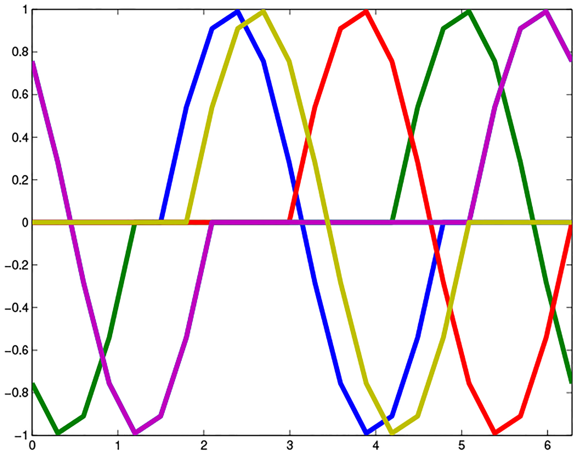
Shifted copies of a function over SO(2)

Next, suppose that we have noisy shifted copies of the function (fig. 5(a)). If we wish to approximate the original function (up to shifts), we would align the noisy copies (fig. 5(b)) and then average them to cancel out the noise (fig. 5(c)). Of course, in order to do this we must somehow recover the correct shifts of all the copies together (up to some global shift). In the following sections, we will use a loss function for different possible pairwise alignment; for each pair of copies, we can define a “compatibility penalty” for different possible alignments, for example (with slight abuse of notation), via the formula

$$f_{i,j}\left(g\right)={\Vert {\phi }_i-g\circ {\phi }_j\Vert }_2^2=\frac{1}{2\pi }{\int }_0^{2\pi }{\left|{\phi }_i\left(\theta \right)-{\phi }_j\left(\theta -g\right)\right|}^{2}d\theta .$$ (24)

An example of such compatibility loss function is given in fig. 6. When the shifts are unknown, the problem of aligning the signals is a NUG (see [2, 1]).

Figure 5:

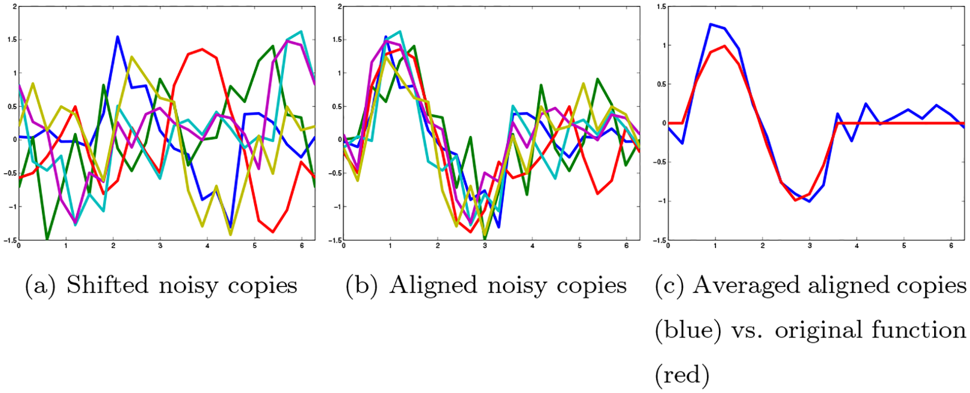
Noisy shifted copies of a function over SO(2)

Figure 6:

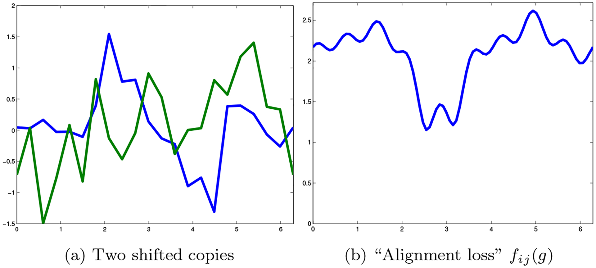
Loss function for alignment of signals

In the heterogeneity problem we have a mixture of prototype signals; in this simplified example, let us assume that we have a mixture of noisy shifted versions of two classes of functions ${\psi }_1$ and ${\psi }_2$, so that each sample is a shifted noisy version of either ${\psi }_1$ or ${\psi }_2$ as illustrated in the example in fig. 7(a). If we knew both the class and shift of each sample, we could divide the samples into two classes, and align them within each class (fig. 7(b),(c)), so that we could average within each class and approximate the two original signals (fig. 7 (d),(e)).

Figure 7:

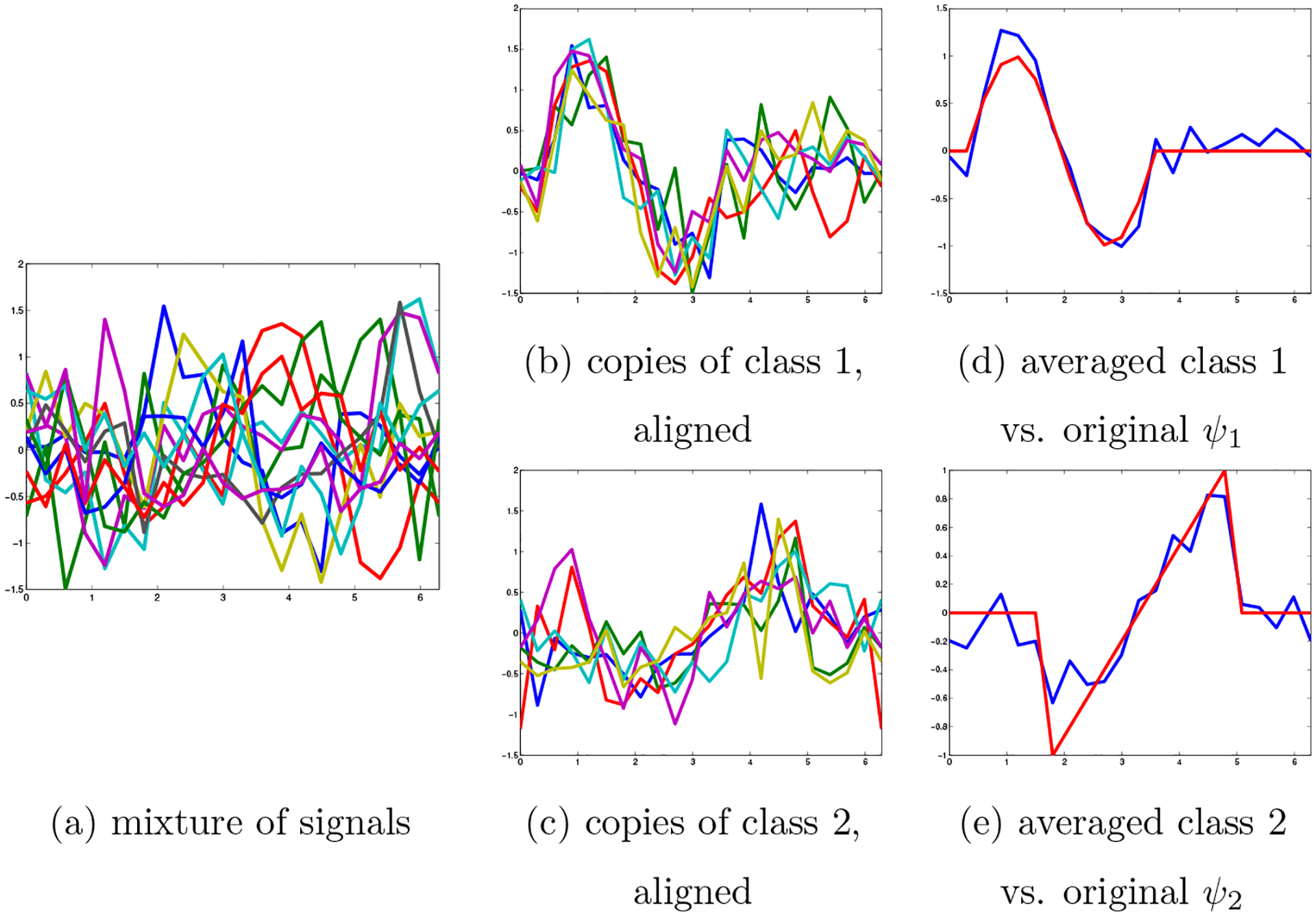
Classification and alignment over SO(2)

We know neither the shift nor the class of the samples; we study the extension of MRA and NUG to this case of alignment in the presence of heterogeneity.

3.2. Problem Formulation

We would like to find the optimal way to divide the samples into $M$ classes, so that we can best align them within each class. More formally, we would like to optimize the rotations and classification together:

$$\underset{\begin{array}{c}{g}_1,\dots ,g_n\in 𝒢\\ a_1,\dots ,a_n\in 0,\mathrm{..},M-1\end{array}}{\text{arg}\text{min}}\sum _{m=0}^{M-1}\sum _{\begin{array}{c}i,j:\\ a_i=m\\ a_j=m\end{array}}{f}_{ij}\left(g_i{g}_j^{-1}\right).$$ (25)

Remark 5. In this formulation, it is typically assumed that the loss $f_{ij}$ is non-negative, and typically larger when $i$ and $j$ do not belong to the same class, so that there is an incentive to distribute the samples among $M$ clusters, and align them within each cluster.

We will also discuss the problem of controlling the distribution to different clusters; for example, we will discuss the case where all the clusters are required to be of equal size:

$$\left|\left\{i:a_i=m\right\}\right|=n/M.$$ (26)

3.3. Ambiguity

In some cases, there is a degree of ambiguity in a solution of a NUG (in addition to the inherent global ambiguity discussed in remark 3). Suppose that $g_1,g_2,\dots ,g_n$ is a solution of the NUG in eq. (18) with the corresponding matrices $X^{\left(0\right)},X^{\left(1\right)},\dots$, and suppose that there exists another solution ${\tilde{g}}_1,{\tilde{g}}_2,\dots ,{\tilde{g}}_n$ with corresponding matrices ${\tilde{X}}^{\left(0\right)},{\tilde{X}}^{\left(1\right)},\dots$ that achieves the same optimization objective. We would be particularly interested in the case where ${\tilde{g}}_1,{\tilde{g}}_2,\dots ,{\tilde{g}}_n$ cannot be obtained by applying some group element to $g_1,g_2,\dots ,g_n$ (the case discussed in remark 3), so that in general $X^{\left(k\right)}\ne {\tilde{X}}^{\left(k\right)}$. In the convex formulation of the problem in eq. (21), if both $X^{\left(0\right)},X^{\left(1\right)},\dots$ and ${\tilde{X}}^{\left(0\right)},{\tilde{X}}^{\left(1\right)},\dots$ are solutions, then so is every convex combination ${\bar{X}}^{\left(0\right)},{\bar{X}}^{\left(1\right)},\dots$ of those solutions, even if there is no “physical” solution ${\bar{g}}_1,{\bar{g}}_2,\dots ,{\bar{g}}_n$ which corresponds to ${\bar{X}}^{\left(0\right)},{\bar{X}}^{\left(1\right)},\dots$.. In some cases, where the form of the ambiguity is known, we can use this property to enforce a solution of a certain form. An example is provided in the next section.

3.4. Reducing k-clustering to a NUG

In this section we discuss the NUG formulation of the problem of clustering vertices in a graph in k communities, to which we refer as k-clustering or k-classification. In particular, we discuss the max-k-cut problem and the balanced version of the problem (where each cluster contains an equal number of vertices). The SDP relaxation of max-k-cut has been studied in [3, 4] and the closely related min-k-cut problem has been studied as a NUG in [2]. For completeness, we present a slightly different formulation and derivation of the max-k-cut problem to illustrate some aspects of the NUG SDP which are useful the remainder of the discussion of alignment and classification. Since $“k”$ is often reserved for denoting indices of irreducible representations, we denote the number of clusters by $M$.

Given an undirected weighted graph $(V,E)$ (e.g. fig. 8(a)), the max-k-cut problem is to divide the vertices of a graph into $M$ clusters (e.g. fig. 8(b)), cutting the most edges between clusters

$$\underset{a_1,\dots ,a_n\in 0,\dots ,M-1}{\text{arg}\text{max}}\sum _{i,j=1}^n\left(1-\delta \left(a_i-a_j\right)\right)w_{ij},$$ (27)

with $w_{ij}$ the weight of the edge between vertices $i$ and $j$. In other words, the problem is to divide the graph into $M$ clusters retaining the minimal sum of edge weights:

$$\underset{a_1,\dots ,a_n\in 0,\dots ,M-1}{\text{arg}\text{min}}\sum _{i,j=1}^n{f}_{ij}\left(a_i-a_j\right),$$ (28)

where $f_{ij}\left(a\right)=w_{ij}\delta \left(a\right)$. We can view the weight of each edge as a measure of incompatibility or “distance,” and attempt to classify the vertices into clusters which are the least incompatible; i.e. the goal is to minimize the sum of intra-cluster weights retained, by finding a clustering that removes as many inter-cluster edges as possible.

Figure 8:

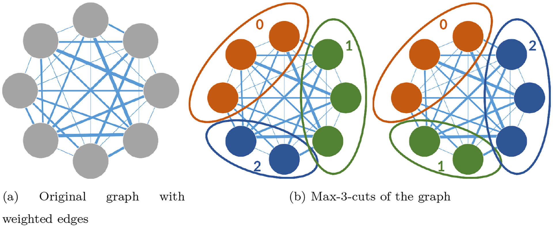
Graph cut and label ambiguity. A graph and equivalent Max-3-cuts, where only the label assigned to each class is changed, without changing the cut.

The following SDP relaxation has been proposed in [3, 4],

$$\begin{array}{lll}\underset{Y}{\text{min}}\hfill & tr\left(WY\right)\hfill & \\ \text{Subject to}\hfill & Y\underset{\_}{\succ }0\hfill & \\ & Y_{ii}=1\hfill & \forall i\hfill \\ & Y_{ij}\ge -\frac{1}{M-1}\hfill & \forall i,j\hfill \end{array}$$ (29)

where $W$ is the matrix of edge weights. In a solution that corresponds to a “physical” solution (a valid classification, rather than, for example, a convex combination of classifications), $Y_{ij}=1$ if $i$ and $j$ are in the same cluster, and $Y_{ij}=-\frac{1}{M-1}$ otherwise. A derivation for the related min-k-cut problem, in the context of NUG, is provided in [2]. We discuss an additional derivation which we will generalize in the following sections.

We consider the group ${\mathbb{Z}}_M$ of cyclic shifts. A function over this group can be written explicitly as a vector of length $M$, indexed $0,1,\dots ,M-1$. We define the function $f_{ij}$ by the following formula

$$f_{ij}={\left(w_{ij},0,0,\dots \right)}^{\top },$$ (30)

where $w_{ij}$ is the weight of the edge between $i$ and $j$. We denote by $a_i$ the class assignment of the $i$ element, so that

$$f_{ij}\left(a_i-a_j\right)=\left\{\begin{array}{lll}0& :& a_i\ne a_j\\ w_{ij}& :& a_i=a_j\end{array}\hspace{1em},\right.$$ (31)

or, in group notation

$$f_{ij}\left(a_i{a}_j^{-1}\right)=\left\{\begin{array}{lll}0& :& a_i{a}_j^{-1}\ne \mathrm{e}\\ w_{ij}& :& a_i{a}_j^{-1}=\mathrm{e}\end{array}\hspace{1em},\right.$$ (32)

where e is the identity element. This $f_{ij}$ is precisely the loss function $f_{ij}$ in eq. (28).

The discrete Fourier transform (DFT) of $f_{ij}$ (with the appropriate choice of normalization) is

$${\hat{f}}_{ij}=\frac{1}{M}{\left(w_{ij},w_{ij},w_{ij},\dots \right)}^{\top }.$$ (33)

These coefficients coincide with the coefficients of the expansion of $f_{ij}$ in the irreducible representation of ${\mathbb{Z}}_M$:

$$f_{ij}\left(a\right)=\sum _{m=0}^{M-1}{\hat{f}}_{ij}\left(m\right)e^{\text{i}2\pi am/M}.$$ (34)

Rewriting the clustering problem eq. (28) as a NUG over ${\mathbb{Z}}_M$ yields

$$\underset{a_1,\dots ,a_n\in {\mathbb{Z}}_M}{\text{arg}\text{min}}\sum _{i,j=1}^n{f}_{ij}\left(a_i{a}_j^{-1}\right),$$ (35)

and substituting eq. (33) and eq. (35) into the block matrix formulation in eq. (18) yields

$$\underset{X^{\left(0\right)},\dots ,X^{(M-1)}}{\mathrm{a}\mathrm{r}\mathrm{g}\mathrm{m}\mathrm{i}\mathrm{n}}{\sum }_{m=0}^{M-1}tr\left({\hat{F}}^{\left(m\right)}{X}^{\left(m\right)}\right)$$ (36)

subject to $X^{\left(m\right)}$ having the structure in eq. (19). The scalar irreducible representations here are ${\eta }_m\left(a\right)=e^{\mathrm{i}2\pi am/k}$, so that for every $m=0,1,\dots ,M-1$, the matrix $X^{\left(m\right)}$ is an $n\times n$ matrix with $X_{ij}^{\left(m\right)}$ in position $i,j$. The matrix ${\hat{F}}^{\left(m\right)}$ is a matrix of the coefficients ${\hat{f}}_{ij}\left(m\right)$ in the DFT of $f_{ij}$; by eq.(33), ${\hat{f}}_{ij}^{\left(m\right)}=w_{ij}/M$, for all $m$. For some solution of the NUG, we have for every pair $i,j$, with $a_i{a}_j^{-1}=a_{ij}$

$$X_{ij}^{\left(m\right)}=e^{\mathrm{i}2\pi a_{ij}m/M},$$ (37)

where we again use $a_{ij}$ as the group elements and the angle.

After writing the problem in the block matrix form, we turn our attention to the convex version of this formulation (see eq. (21)). In particular, we discuss the ambiguity in the solution, which results in convex combinations of equivalent solutions, as discussed in section 3.3. Obviously, the solution to eq. (28) is unique at most up to any permutation (and not only cyclic shifts) of the labels assigned to each class. For example, Class 1 can be renamed Class 2 and vice versa, without changing the graph cut, as illustrated in fig. 8(b). In other words, the loss function $f_{ij}\left(a_i{a}_j^{-1}\right)$ depends only on whether or not $i$ and $j$ are in the same class, so it is invariant to permutations: for any permutation $\sigma$,

$$\sum _{i,j=1}^n{f}_{ij}\left(a_i{a}_j^{-1}\right)=\sum _{i,j=1}^n{f}_{ij}\left(\sigma \left(a_i\right){\left(\sigma \left(a_j\right)\right)}^{-1}\right).$$ (38)

It follows that in the convexified formulation we can average all the different permutations, as discussed in section 3.3. If $i$ and $j$ are assigned to the same class in the solution, then $a_i=a_j$ so $a_{ij}=a_i{a}_j^{-1}=\mathrm{e}$ (or in integer notation $a_i-a_j=0$) and by eq. (37)

$$X_{ij}^{\left(0\right)}=X_{ij}^{\left(1\right)}=\dots =X_{ij}^{(M-1)}=1.$$ (39)

However, if $i$ and $j$ are not assigned to the same class in the solution, we can average all the solutions for all permutations, where the solution for a permutation $\sigma$ is

$$X_{ij}^{\left(m\right)}=e^{\mathrm{i}2\pi \left(\sigma \left(a_i\right){\left(\sigma \left(a_j\right)\right)}^{-1}\right)m/M}=e^{\mathrm{i}2\pi \left(\sigma \left(a_i\right)-\sigma \left(a_j\right)\right)m/M}.$$ (40)

A simple computation yields the averaged (equally weighted convex combination) solution for all $m>0$, when $i$ and $j$ are not assigned to the same class,

$${\overline{X}}_{ij}^{\left(m\right)}=\frac{1}{M-1}\sum _{a=1}^{M-1}{e}^{\text{i}2\pi am/M}=-\frac{1}{M-1}.$$ (41)

In other words, $X^{\left(0\right)}$ is the all-ones matrix, and the matrices for all $m>0$ are equal:

$$X^{\left(1\right)}=X^{\left(2\right)}=\dots =X^{\left(M-1\right)},$$ (42)

with the element $X_{ij}^{\left(m\right)}$ of these matrices with $m>0$:

$$X_{ij}^{\left(m\right)}=\left\{\begin{array}{ll}1& ,\hspace{1em}\text{if }i \text{and }j \text{are in the same class},\\ -\frac{1}{M-1}& ,\hspace{1em}\text{otherwise.}\end{array}\right.$$ (43)

Since $X_{ij}^{\left(0\right)}=1$ is fixed, it can be ignored in the loss term of eq. (36), so the optimization is reduced to

$$\underset{X^{\left(1\right)},\dots ,X^{\left(M-1\right)}}{\text{arg}\text{min}}\sum _{m=1}^{M-1}tr\left({\hat{F}}^{\left(m\right)}{X}^{\left(m\right)}\right).$$ (44)

Using eq. (42) and eq. (33), the optimization is further reduced to

$$\underset{X^{\left(1\right)}}{\mathrm{a}\mathrm{r}\mathrm{g}\mathrm{m}\mathrm{i}\mathrm{n}}\left((M-1)tr\left({\hat{F}}^{\left(1\right)}{X}^{\left(1\right)}\right)\right),$$ (45)

which is scaled to

$$\underset{X^{\left(1\right)}}{\mathrm{a}\mathrm{r}\mathrm{g}\mathrm{m}\mathrm{i}\mathrm{n}}\left(tr\left({\hat{F}}^{\left(1\right)}{X}^{\left(1\right)}\right)\right).$$ (46)

Setting $X^{\left(1\right)}=Y$, we have the optimization term in eq. (29), with the other conditions in eq. (29) following from the derivation above.

3.5. Controlling Cluster Size or Distributions

The purpose of this section is to extend the NUG framework by adding constraints on the distribution of solutions over the group.

In some cases it is useful to restrict the clusters in a graph cut problem to be of equal size (for example, see discussion of min-k-cut in [32]), i.e.

$$\left|\left\{i:a_i=m\right\}\right|=n/M.$$ (47)

The NUG formulation does not have a mechanism to enforce such a constraint. We first consider the extension of the NUG in eq. (29) for the max-k-cut problem to the case of balanced cluster size. We add the constraint that for $m>0$,

$$\sum _j{X}_{ij}^{\left(m\right)}=0\hspace{1em}\forall i$$ (48)

(for $m=0$, the matrix $X^{\left(0\right)}$ is the trivial all ones matrix). Indeed, for any valid balanced solution, every vertex $i$ has $n/M$ vertices (including itself) in the same cluster, and for these vertices $X_{ij}^{\left(m\right)}=1$; every vertex also has $\frac{n}{M}(M-1)$ vertices in different classes, for these vertices $X_{ij}^{\left(m\right)}=-\frac{1}{M-1}$. Therefore, the sum of these elements is 0. This solution resembles the algorithm proposed in [32].

This idea is a special case of a more general framework that enforces constant distribution over the group by enforcing eq. (48). The strict constraint on the distribution can be relaxed to an approximation, and therefore extended beyond discrete groups by relaxing the condition to one of the following constraints

$${\left|\sum _j{X}_{ij}^{\left(m\right)}\left(q\right)\right|}^2\le w\left(m\right)\hspace{1em}\forall i,$$ (49)

$${\left|\sum _{ij}{X}_{ij}^{\left(m\right)}\left(q\right)\right|}^2\le w\left(m\right),$$ (50)

$$\sum _i{\left|\sum _j{X}_{ij}^{\left(m\right)}\left(q\right)\right|}^2\le w\left(m\right),$$ (51)

or by adding a similar constraint as a regularizer in the optimization (with the obvious extension where the irreducible representation $X_{ij}^{\left(m\right)}$ is a matrix). This approach, which views the irreducible representations and their sum as an approximation of the Haar measure of the group (or appropriate variation when a prior is available), will be discussed in more detail in a future paper.

3.6. The Direct Product of Alignment and Classification (Product NUG)

The purpose of this section is to formulate the problem of simultaneous alignment and classification as a NUG. We revisit eq. (25) and rewrite the summation in the optimization:

$$\sum _{m=0}^{M-1}\sum _{\begin{array}{c}i,j:\\ a_i=m\\ a_j=m\end{array}}{f}_{ij}\left(g_i{g}_j^{-1}\right)=\sum _{i,j=1}^n\delta \left(a_i,a_j\right)f_{ij}\left(g_i{g}_j^{-1}\right),$$ (52)

where

$$\delta \left(a_i,a_j\right)=\left\{\begin{array}{lll}1& :& a_i=a_j\\ 0& :& \text{otherwise}\end{array}.\right.$$ (53)

With a small abuse of notation, we rewrite the class labels $a_1,\dots ,a_n$ as elements in ${\mathbb{Z}}_M$; the expression $a_i=a_j$ can also be written as $a_i{a}_j^{-1}=e$ (where $e$ is the identity element of ${\mathbb{Z}}_M$), so, we can also write eq. (53) as:

$$\delta \left(a_i,a_j\right)=\delta \left(a_i{a}_j^{-1}\right)=\left\{\begin{array}{lll}1& :& a_i{a}_j^{-1}=e\\ 0& :& \text{otherwise.}\end{array}\right.$$ (54)

We introduce the function ${\tilde{f}}_{ij}:𝒢\times {\mathbb{Z}}_M\to \mathbb{R}$, defined as

$${\tilde{f}}_{ij}\left(\left(g,a\right)\right)=f_{ij}\left(g\right)\delta \left(a\right).$$ (55)

Using the identity eq. (12), we obtain

$${\tilde{f}}_{ij}\left(\left(g_i,a_i\right){\left(g_j,a_j\right)}^{-1}\right)={\tilde{f}}_{ij}\left(\left(g_i{g}_j^{-1},a_i{a}_j^{-1}\right)\right),$$ (56)

and observe that ${\tilde{f}}_{ij}\left(\left(g_i,a_i\right){\left(g_j,a_i\right)}^{-1}\right)$ is now simply a function over the compact group $𝒢\times {\mathbb{Z}}_M$. Therefore, the expression in eq. (25) is reduced to the the explicit form of a NUG

$$\underset{\left(g_1,a_1\right),\dots ,\left(g_n,a_n\right)\in 𝒢\times {\mathbb{Z}}_M}{\text{arg}\text{min}}\sum _{i,j}{\tilde{f}}_{ij}\left(\left(g_i,a_i\right){\left(g_j,a_j\right)}^{-1}\right).$$ (57)

The block matrix formulation eq. (18) of this product NUG is

$$\underset{\left(g_1,a_1\right),\dots ,\left(g_n,a_n\right)\in 𝒢\times {\mathbb{Z}}_M}{\text{arg}\text{min}}\sum _{k=0}^{\infty }\sum _{m=0}^{M-1}tr\left({\hat{F}}^{\left(k,m\right)}{X}^{\left(k,m\right))}\right)$$ (58)

Where,

$$\begin{array}{c}{X}^{\left(k,m\right)}=\left[\begin{array}{c}{\psi }_{k,m}\left(\left(g_1,a_1\right)\right)\\ ⋮\\ {\psi }_{k,m}\left(\left(g_n,a_n\right)\right)\end{array}\right]{\left[\begin{array}{c}{\psi }_{k,m}\left(\left(g_1,a_1\right)\right)\\ ⋮\\ {\psi }_{k,m}\left(\left(g_n,a_n\right)\right)\end{array}\right]}^{\text{*}},\\ {\hat{F}}^{\left(k,m\right)}=d_{km}\left[\begin{array}{ccc}{\hat{f}}_{11}\left(k,m\right)& \cdots & {\hat{f}}_{n1}\left(k,m\right)\\ ⋮& \ddots & ⋮\\ {\hat{f}}_{1n}\left(k,m\right)& \cdots & {\hat{f}}_{nn}\left(k,m\right)\end{array}\right],\end{array}$$ (59)

with ${\hat{f}}_{ij}(k,m)$ the Fourier coefficient of ${\tilde{f}}_{ij}$ corresponding to the irreducible representation ${\psi }_{k,m}$, and $d_{km}$ the dimensionality of that irreducible representation. The irreducible representations ${\psi }_{k,m}$ of $𝒢\times {\mathbb{Z}}_M$ are enumerated in table 4; they are referenced by two indices, $k=\mathrm{0,1},\dots$ and $m=\mathrm{0,1},\dots ,M-1$.

As in the general discussion of NUG, we are interested in the convex relaxation of eq. (58):

$$\underset{{\left\{X^{\left(k,m\right)}\right\}}_{k,m}}{\text{arg}\text{min}}\sum _{m=0}^{M-1}\sum _{k=0}^{\infty }tr\left({\hat{F}}^{\left(k,m\right)}{X}^{\left(k,m\right)}\right)$$ (60)

where the solution matrices $X^{(k,m)}$ are in the convex hull of the matrices defined in eq. (59).

The relaxation of the form eq. (22) is

$$\begin{array}{lll}\underset{X^{(k,m)}}{\mathrm{m}\mathrm{a}\mathrm{x}\mathrm{i}\mathrm{m}\mathrm{i}\mathrm{z}\mathrm{e}}& \sum _{m=0}^{M-1}\sum _{k=0}^{\infty }tr\left({\hat{F}}^{(k,m)}{X}^{(k,m)}\right)& \\ \text{subject to}& X^{(k,m)}⪰0& \forall k,m\\ & X_{ii}^{(k,m)}=1& \forall k,m,i\\ & \sum _{k,m}tr\left({\psi }_{k,m}^{*}\left(\right(g,a\left)\right)X_{ij}^{(k,m)}\ge 0\right)& \forall i,j,\forall (g,a)\in 𝒢\times {\mathbb{Z}}_M\\ & X_{ij}^{\left(\mathrm{0,0}\right)}=1& \forall i,j\\ & X_{ij}^{(k,m)}\ge -\frac{1}{M-1}& \forall m>0,\forall i,j.\end{array}$$ (61)

In the following sections, we turn our attention to the ambiguities and symmetries in $X^{(k,m)}$ of the convexified formulation eq. (60).

3.7. The 0 Order Representation of Alignment, and the Clustering Label Ambiguity

As discussed in section 3.3, when there is ambiguity in the solution of the NUG, it is manifested as convex combinations of solutions in the covexified formulation eq. (60). As discussed in section 3.4, there is ambiguity in the assignment of class labels which leads to symmetries in the NUG for the clustering problem.

We observe that the irreducible representations ${\psi }_{0,m}$ of $𝒢\times {\mathbb{Z}}_M$, enumerated in the first row of table 4, are simply the irreducible representations of ${\mathbb{Z}}_M$ which appear in the max-k-cut problem, as are the coefficients of the expansion of $f_{ij}$. Therefore, the same argument used in section 3.4 can be used here to identify the desired form of the first row in the solution of the convex simultaneous alignment and classification problem eq. (60). In fact, the same argument applies to all rows, which can be averaged in the same way; the form of the averaged solution of each block $X_{ij}^{(k,m)}$ is summarized in table 5, for the two cases: either $i$ and $j$ are in the same class (a), or they are in different classes (b).

Table 5:

The desired form of blocks $X_{ij}^{(k,m)}$ of $X^{(k,m)}$, corresponding to (a) same, and (b) distinct classes

$\text{(a) }{a}_i=a_j$					$\text{(b) }{a}_i\ne a_j$
$X^{(k,m)}$	$\mathit{m}=0$	$\mathit{m}=1$	$\cdots$	$\mathit{m}=\mathit{M}-1$	$X^{(k,m)}$	$\mathit{m}=0$	$\mathit{m}=1$	$\cdots$	$\mathit{m}=\mathit{M}-1$
$k=0$	$1$	$1$	$\cdots$	$1$	$k=0$	$1$	$-\frac{1}{M-1}$	$\cdots$	$-\frac{1}{M-1}$
$k=1$	$X_{ij}^{(1,0)}$	$X_{ij}^{(1,0)}$	$\cdots$	$X_{i,j}^{(1,0)}$	$k=1$	$X_{ij}^{(1,0)}$	$-\frac{X_{ij}^{(1,0)}}{M-1}$	$\cdots$	$-\frac{X_{ij}^{(1,0)}}{M-1}$
$k=2$	$X_{i,j}^{(2,0)}$	$X_{i,j}^{(2,0)}$	$\cdots$	$X_{i,j}^{(2,0)}$	$k=2$	$X_{i,j}^{(2,0)}$	$-\frac{X_{i,j}^{(2,0)}}{M-1}$	$\cdots$	$-\frac{X_{i,j}^{(2,0)}}{M-1}$
$⋮$	$⋮$	$\ddots$	$⋮$		$⋮$	$⋮$	$\ddots$	$⋮$

3.8. Inter-Class Invariance

In addition to the class label ambiguity, there is another type of ambiguity which emerges in the simultaneous clustering and alignment product NUG. We observe that the solution is invariant to a $𝒢$ group action on one class (without applying the same action to the other classes, so this is not a group action of $𝒢\times 𝒜$).

Lemma 1. Let $a_1,\dots ,a_n\in {\mathbb{Z}}_M,g_1,\dots ,g_n\in 𝒢$ and ${\tilde{g}}_1,\dots ,{\tilde{g}}_n\in 𝒢$. Suppose that a $\in {\mathbb{Z}}_M$ and $g\in 𝒢$ are some arbitrary class and rotation, and suppose that

$${\tilde{g}}_i=\left\{\begin{array}{lll}{g}_{i}g& :& a_i=a\\ g_i& :& \mathit{\text{otherwise}}.\end{array}\right.$$ (62)

Then, the objective value in eq. (25) is the same for $g_1,\dots ,g_n\in 𝒢$ and ${\tilde{g}}_1,\dots ,{\tilde{g}}_n\in 𝒢$:

$$\sum _{m=0}^{M-1}\sum _{\begin{array}{c}i,j:\\ a_i=m\\ a_j=m\end{array}}{f}_{ij}\left(g_i{g}_j^{-1}\right)=\sum _{m=0}^{M-1}\sum _{\begin{array}{c}i,j:\\ a_i=m\\ a_j=m\end{array}}{f}_{ij}\left({\tilde{g}}_i{\tilde{g}}_j^{-1}\right).$$ (63)

In other words, if $a_1,\dots ,a_n,g_1,\dots ,g_n$ is a solution of eq. (25), then so is $a_1,\dots ,a_n,{\tilde{g}}_1,\dots ,{\tilde{g}}_n$.

Proof. For any $m\ne a$ (the clusters that have not been rotated), ${\tilde{g}}_i=g_i$, so that

$$\sum _{\begin{array}{c}i,j:\\ a_i=m\\ a_j=m\end{array}}{f}_{ij}\left({\tilde{g}}_i{\tilde{g}}_j^{-1}\right)=\sum _{\begin{array}{c}i,j:\\ a_i=m\\ a_j=m\end{array}}{f}_{ij}\left(g_i{g}_j^{-1}\right).$$ (64)

For $m=a$, we have

$$f_{ij}\left({\tilde{g}}_i{\tilde{g}}_j^{-1}\right)=f_{ij}\left(\left(g_{i}g\right){\left(g_{j}g\right)}^{-1}\right)=f_{ij}\left(g_{i}g{g}^{-1}{g}_j^{-1}\right)=f_{ij}\left(g_i{g}_j^{-1}\right)$$ (65)

so that eq. (64) holds for $m=a$ as well. □

It follows that when $a_i\ne a_j$, we may average over all inter-class rotations. By eq. (6), using the Haar measure for the possible alignments yields 0 for all elements with $k\ne 0$. The form of the averaged solution of each block $X_{ij}^{(k,m)}$ is summarized in table 6, for the two cases: either $i$ and $j$ are in the same cluster, or they are in different clusters.

Table 6:

The desired form of blocks $X_{ij}^{(k,m)}$ of $X^{(k,m)}$, after averaging inter-class rotations (lemma 1)

$\text{(a) }{a}_i=a_j$					$\text{(b) }{a}_i\ne a_j$
$X^{(k,m)}$	$\mathit{m}=0$	$\mathit{m}=1$	$\cdots$	$\mathit{m}=\mathit{M}-1$	$X^{(k,m)}$	$\mathit{m}=0$	$\mathit{m}=1$	$\cdots$	$\mathit{m}=\mathit{M}-1$
$k=0$	$1$	$1$	$\cdots$	$1$	$k=0$	$1$	$-\frac{1}{M-1}$	$\cdots$	$-\frac{1}{M-1}$
$k=1$	$X_{ij}^{(1,0)}$	$X_{ij}^{(1,0)}$	$\cdots$	$X_{i,j}^{(1,0)}$	$k=1$	$0$	$0$	$\cdots$	$0$
$k=2$	$X_{i,j}^{(2,0)}$	$X_{i,j}^{(2,0)}$	$\cdots$	$X_{i,j}^{(2,0)}$	$k=2$	$0$	$0$	$\cdots$	$0$
$⋮$	$⋮$	$\ddots$	$⋮$		$⋮$	$⋮$	$\ddots$	$⋮$

4. Algorithms

Substituting the results of section 3.6 into eq. (22) we obtain the following SDP:

$$\begin{array}{lll}\underset{{\left\{X^{\left(k,m\right)}\right\}}_{k,m}}{\text{arg}\text{min}}& {\sum }_{k=0}^{\infty }{\sum }_{m=0}^{M-1}tr\left({\widehat{F}}^{\left(k,m\right)}{X}^{\left(k,m\right)}\right)& \\ \text{subject to}& X^{\left(k,m\right)}\succcurlyeq 0& \forall k,m\\ & X_{ii}^{\left(k,m\right)}=I_{d_k\times d_k}& \forall k,m,i\\ & {\sum }_{k=0}^{\infty }{\sum }_{m=0}^{M-1}{d}_{k}tr\left({\psi }_{k,m}^{\text{*}}\left(\left(g,a\right)\right)X_{ij}^{\left(k\right)}\right)\ge 0& \forall i,j\\ & & \forall g,a\in 𝒢\times {\mathbb{Z}}_M\\ & X_{ij}^{\left(0,0\right)}=1& \forall i,j\end{array}$$ (66)

The coefficient in the matrix ${\hat{F}}^{(k,m)}$ can be obtained from the original alignment problem, when no clustering is required; suppose that the coefficients in that problem are ${\hat{F}}^{\left(k\right)}$, then for all $k$ and $m$, the coefficients ${\hat{F}}^{(k,m)}$ are

$${\hat{F}}^{(k,m)}=\frac{1}{M}{\hat{F}}^{\left(k\right)}.$$ (67)

We observe that due to the structure discussed in sections 3.7 and 3.8, regardless of whether $a_i=a_j$ or $a_i\ne a_j$,

$$\begin{array}{ll}{X}^{(0,m)}=X^{\left(\mathrm{0,1}\right)}& \forall m\ne 0\\ X^{(k,m)}=X^{(k,0)}& \forall k\ne 0,\forall m.\end{array}$$ (68)

Taking these observations into account, eq. (66) is reduced to

$$\begin{array}{lll}\underset{X^{\left(k,m\right)}}{\text{arg}\text{min}}& {\sum }_{m=0}^{M-1}{\sum }_{k=0}^{\infty }tr\left({\hat{F}}^{\left(k,m\right)}{X}^{\left(k,m\right)}\right)& \\ \text{subject to}& X^{\left(0,m\right)}=X^{\left(0,1\right)}& \forall m\ne 0\\ & X^{\left(k,m\right)}=X^{\left(k,0\right)}& \forall k\ne 0\hspace{1em},\hspace{1em}\forall m\\ & X_{ij}^{\left(0,m\right)}\ge -\frac{1}{M-1}& \forall m>0\hspace{1em},\hspace{1em}\forall i,j\\ & X^{\left(k,m\right)}\underset{\_}{\succ }0& \forall k,m\\ & X_{ii}^{\left(k,m\right)}=1& \forall k,i\\ & {\sum }_{k,m}tr\left({\psi }_{k,m}^{\text{*}}\left(\left(g,a\right)\right)X_{ij}^{\left(k,m\right)}\right)\ge 0& \forall i,j,\forall \left(g,a\right)\in 𝒢\times {\mathbb{Z}}_M\\ & X_{ij}^{\left(0,0\right)}=1& \forall i,j.\end{array}$$ (69)

In fact, the requirement for non-negativity over $𝒢\times {\mathbb{Z}}_M$ is redundant, due to the following lemma.

Lemma 2. Suppose that $a\ne e$ (where $e$ is the identity element of ${\mathbb{Z}}_M$). If the other constraints in eq. (69) are satisfied, then for all $i,j$,

$$\sum _{k,m}tr\left({\rho }_{k,m}^{\text{*}}\left(\left(g,a\right)\right)X_{ij}^{\left(k,m\right)}\right)\ge 0$$ (70)

for all $g\in 𝒢$ and all $a\ne e$.

Proof. Due to the other constraints in eq. (69), for all $k>0$, we have $X^{(k,0)}=X^{(k,1)}=\dots =X^{(k,m)}$, so that for all $k>0$

$$\sum _{m=0}^{M-1}tr\left({\psi }_{k,m}^{\text{*}}\left(\left(g,a\right)\right)X_{ij}^{\left(k,m\right)}\right)=tr\left({\rho }_k^{\text{*}}\left(g\right)X_{ij}^{\left(k,0\right)}\right)\sum _{m=0}^{M-1}{\eta }_m\left(a\right)=0$$ (71)

where the last step is due to the fact that ${\sum }_{m=0}^{M-1}{\eta }_m\left(a\right)=0$ for $a$ that are not the identity.

For $k=0$, we have $X_{ij}^{\left(\mathrm{0,0}\right)}=1$ and $-\frac{1}{M-1}\le X^{(0,m)}\le 1$, so that

$$\sum _{m=0}^{M-1}tr\left({\psi }_{0,m}^{\text{*}}\left(\left(g,a\right)\right)X_{ij}^{\left(0,m\right)}\right)=1+\sum _{m=1}^{M-1}{\eta }_m\left(a\right)X_{ij}^{\left(0,m\right)}\ge 1-\left(M-1\right)/\left(M-1\right)=0$$ (72)

Using this lemma, eq. (69) is reduced to

$$\begin{array}{lll}\underset{X^{\left(k,m\right)}}{\text{arg}\text{min}}& {\sum }_{m=0}^{M-1}{\sum }_{k=0}^{\infty }tr\left({\widehat{F}}^{\left(k,m\right)}{X}^{\left(k,m\right)}\right)& \\ \text{subject to}& X^{\left(0,m\right)}=X^{\left(0,1\right)}& \forall m>1\\ & X^{\left(k,m\right)}=X^{\left(k,0\right)}& \forall k\ne 0\\ & X_{ij}^{\left(0,m\right)}\ge -\frac{1}{M-1}& \forall m>0,\forall i,j\\ & X^{\left(k,m\right)}\succcurlyeq 0& \forall k,m\\ & X_{ii}^{\left(k,m\right)}=1& \forall k,i\\ & {\sum }_{k,m}tr\left({\rho }_{k,m}^{\text{*}}\left(\left(g,e\right)\right)X_{ij}^{\left(k,m\right)}\right)\ge 0& \forall i,j,\forall g\in 𝒢\\ & X_{ij}^{\left(0,0\right)}=1& \forall i,j\end{array}$$ (73)

where $e$ is the identity element of ${\mathbb{Z}}_M$.

4.1. Controlling Class Size

When the size of the classes is known to be equal, the constraint eq. (48) of section 3.5 is added to the SDP. Considering all the symmetries, the constraint takes the form

$$\sum _j{X}_{ij}^{\left(0,1\right)}=0\hspace{1em}\forall i.$$ (74)

4.2. Variables and Constraints Accounting

The purpose of this section is to discuss the number of free variables remaining in the formulation eq. (73), and the number of constraints. We note that the only remaining matrix variables are $X^{\left(\mathrm{0,1}\right)}$ and $X^{\left(\mathrm{1,0}\right)},X^{\left(\mathrm{2,0}\right)},X^{\left(\mathrm{3,0}\right)},\dots$ The matrix $X^{\left(\mathrm{0,0}\right)}$ is the trivial all ones matrix, and every other matrix is set to be equal to the appropriate matrix of those listed above (see eq. 68). We observe that the matrix $X^{\left(\mathrm{0,1}\right)}$ has exactly the same form as the matrix $Y$ in the max-cut classification SDP, and the constrains on it are similar. The matrices $X^{\left(\mathrm{1,0}\right)},X^{\left(\mathrm{2,0}\right)},X^{\left(\mathrm{3,0}\right)}$.. have the same form as the matrices $X^{\left(1\right)},X^{\left(2\right)},X^{\left(3\right)},\dots$ in the alignment problem, and also have similar constraints.

Suppose that the overall number of matrix elements $X_{i.j}^{\left(k\right)}$ (summing over all $k$) for each pair $i,j$ in the irreducible representation for alignment is $\kappa$ (if the expansion is truncated at $K$ representations, the number of elements in the case of SO(2) is $O\left(k\right)$ and in the case of SO(3) it is $\left.O\left(k^3\right)\right)$, and suppose that the number of elements in the irreducible representations for classification is the number of classes $M$. Then, there would be overall approximately $\kappa M$ matrix elements in the matrices $X_{i.j}^{(k,m)}$ for all $k$ and $m$ in the formulation in eq. (66). Instead, the formulation in eq. (73) implies that the remaining variables are $X_{i.j}^{(k,0)}$ and $X_{i.j}^{\left(\mathrm{0,1}\right)}$, so that the overall number of matrix elements is $\kappa +1(\kappa$ variables in $X_{i.j}^{(k,0)}$ and one in $X_{i.j}^{\left(\mathrm{0,1}\right)}$). In other words, the number of free variables and constraints in eq. (73) is smaller than the straightforward formulation that does not take the symmetries into acount.

5. Experimental Results

In this section we present experiments with the simplified case of alignment and clustering of noisy functions over SO(2) (also discussed in section 3.1). We generated 4 complex valued prototype functions over $\mathrm{S}\mathrm{O}\left(2\right)$, the functions are low-bandwidth, represented by 11 coefficients in the Fourier domain. For each prototype function we generated 15 copies, each copy was shifted randomly on SO(2), and random noise was added to each of the shifted copies, yielding a dataset ${\left\{s_i\right\}}_{i=1}^n$ of $n=60$ signals. The problem is now to align and cluster the signals in the dataset.

We implemented the SDP in eq. (73) with balanced classes (eq. (74)) in Matlab, using CVX [33, 34]. For every pair of signals $s_i$ and $s_j$ we compute $f_{ij}$:

$$f_{ij}\left(g\right)=∥s_i-g\circ s_j∥,$$ (75)

where $g\circ s_j$ is the signal $s_j$ rotated by $g$. The rotation is implemented by multiplication by the appropriate phase in the Fourier domain. We construct the $n\times n$ matrices of coefficients ${\hat{F}}^{\left(k\right)}$ (the matrices for MRA without classification); the elements in the $i,j$ position in the $k$ matrix is the $k$ element in the DFT of $f_{ji}$.

$${\hat{f}}_{ij}^{(\cdot )}=ℱ\left(f_{ji}\right).$$ (76)

The non-negativity constraint is implemented using the Fejér kernel (see [2]).

To study the performance of the algorithm, we examine the classification performance, which we can compare to a benchmark clustering method based on shift-invariant signatures. The auto-correlation and bispectrum [35] of signals are invariant to rotations; therefore, in the absence of noise, we can compute the auto-correlation or bispectrum of each signal in our dataset, and use these as signatures by which to cluster. In the presence of noise, these signatures are distorted, leading to possible errors in clustering. We computed the bispectrum of each signal in the dataset and also solved the SDP for the product NUG of this dataset. In the case of low noise, the classification can be read directly from the matrix $X^{\left(\mathrm{0,1}\right)}$, however, as the noise increases, a rounding procedure is required to recover an approximate classification based on the output of the SDP. For simplicity, we used the simple k-means to cluster the signals: first by the bispectral signature of each signal, and then by the columns of the matrix $X^{(0,1)}$ obtained by the SDP (as a simple rounding method for the SDP). For simplicity, we did not enforce equal cluster sizes in the k-means. We measured the fraction of signals that were misclassified (the clusters are recovered only up to permutation: even if the k-means find the correct clusters, the class labels are assigned arbitrarily. We computed the minimum error over all permutations of class labels). This experiment examines only the classification properties of the algorithm, but given a good classification the problem is reduced to the NUG of alignment within each class. Special cases of alignment problems allow specialized rounding procedures using the output of this algorithm directly.

We repeated the experiment 20 times for every noise level. The results are presented in fig. 9. We experimented with both auto-correlation and bispectrum; since the results were very similar in the two cases we present the results for bispectrum here. The experiment demonstrates that the product NUG achieves considerably better classification results in the presence of noise.

Figure 9:

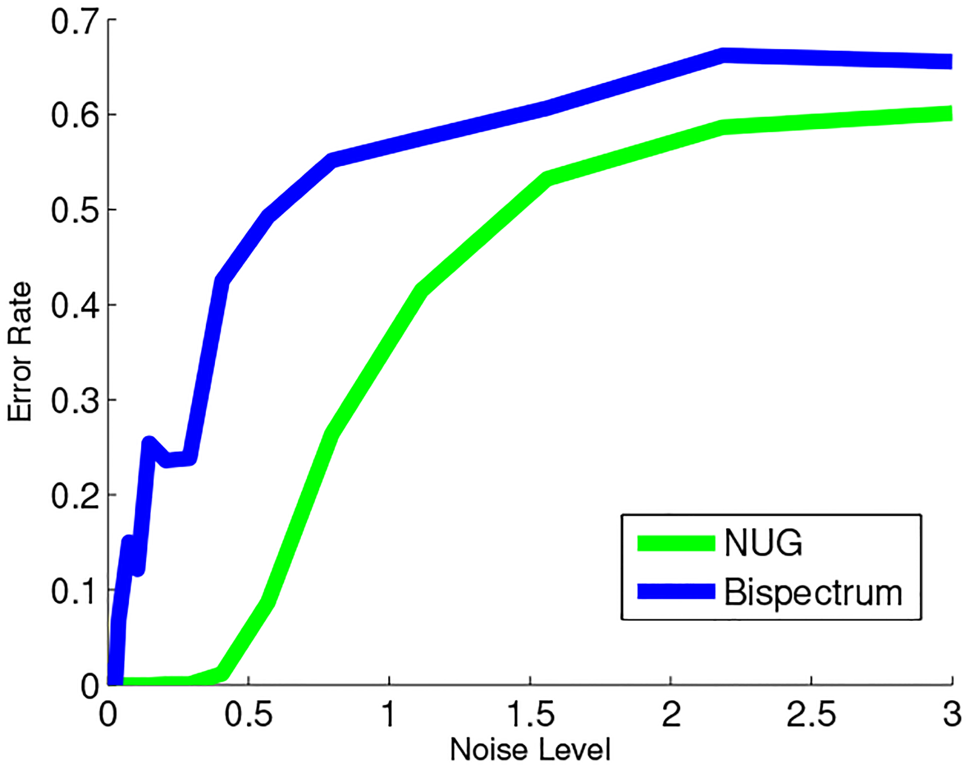
Classification error vs. noise level, 4 balanced clusters

Remark 6. In the cryo-EM problem, the images which we wish to align are different projections of the molecule $𝒳$. While bispectrum and auto-correlation have been used to find images from the same plane (see [36]), these signatures are not invariant to projections. Therefore, in the cryo-EM problem, these signatures cannot be used for classification, so they do not provide an alternative for the product NUG discussed here.

In other words, although the product NUG achieves better results than invariant signature based clustering in these experiments, its true importance is in cases where such alternative methods cannot be used. An implementation of the NUG for alignment over SO(3) in the special case of cryo-EM (even without classification) was not yet avialble at the time of writing this paper.

6. Summary and Future Work

The problem of simultaneous alignment and classification has been formulated as a non-unique game, and an algorithm has been presented for solving a convex relaxation of the problem. The algorithm has been demonstrated for the case of simultaneous alignment and classification of mixed signals over SO(2); and it is currently being adapted for the heterogeneity problem of cryo-EM. It should be noted that SDPs like the one proposed here are difficult to scale using off-the-shelf solvers to very large problems, such as alignment of hundreds of thousands of images produced in modern cryo-EM experiments. Nevertheless, special purpose solvers provide more scalability, the SDPs offer certificates of global optimality of solutions found using other approaches in some circumstances, they provide a benchmark for approximate optimizations, and they can be applied to reduced datasets (e.g. class averages of images). Furthermore, the approach can be used with other recent methods for optimization over groups.

The approach discussed here can be generalized to the case of continuous heterogeneity, where the molecules are not classified to distinct classes, but rather lie on a continuum of states that can be parametrized (alternatively, the states are distinct, but related to some degree). In this case, we follow similar ideas to those in this paper, however there are some additional details that require considerations in the choice of underlying groups and the structure of $f_{ij}$; this case will be discussed in more detail in a future paper.

As discussed in section 3.5, there are several variations of the control over the size of clusters. Furthermore, the same ideas can be used to control the distribution of the recovered rotation angles (for example, when the images can be assumed to come from approximately uniform distribution over SO(3)).

Table 1:

Table of Notation

$A^{\ast }$	the complex conjugate transpose of the matrix $A$
${\mathbb{Z}}_M$	the cyclic group of order $M$
$𝒢\times 𝒜$	the direct product between group $𝒢$ and group $𝒜$
$g\circ f$	the action of $g\in 𝒢$on a function$f\in L^2(𝒴):(g\circ f)(x)=f\left(g^{-1}x\right)$
$tr(A)$	the trace of the matrix $A$
$A\otimes B$	the Kronecker (tensor) product of the matrix A and the matrix $B$

References

- [1].Bandeira AS, Charikar M, Singer A, Zhu A, Multireference alignment using semidefinite programming, in: Proceedings of the 5th conference on Innovations in theoretical computer science, ACM, 2014, pp. 459–470. [Google Scholar]
- [2].Bandeira AS, Chen Y, Singer A, Non-unique games over compact groups and orientation estimation in cryo-em, arXiv preprint arXiv:1505.03840. [DOI] [PMC free article] [PubMed] [Google Scholar]
- [3].Goemans MX, Williamson DP, Improved approximation algorithms for maximum cut and satisfiability problems using semidefinite programming, Journal of the ACM (JACM) 42 (6) (1995) 1115–1145. [Google Scholar]
- [4].Frieze A, Jerrum M, Improved approximation algorithms for max k-cut and max bisection, in: Integer Programming and Combinatorial Optimization, Springer, 1995, pp. 1–13. [Google Scholar]
- [5].Frank J, Three-dimensional electron microscopy of macromolecular assemblies: visualization of biological molecules in their native state, Oxford University Press, 2006. [Google Scholar]
- [6].van Heel M, Gowen B, Matadeen R, Orlova EV, Finn R, Pape T, Cohen D, Stark H, Schmidt R, Schatz M, et al. , Single-particle electron cryo-microscopy: towards atomic resolution, Quarterly reviews of biophysics 33 (04) (2000) 307–369. [DOI] [PubMed] [Google Scholar]
- [7].Scheres S, RELION: Implementation of a Bayesian approach to cryo-EM structure determination, J. Struct. Biol 180 (3) (2012) 519–530. doi: 10.1016/j.jsb.2012.09.006 [DOI] [PMC free article] [PubMed] [Google Scholar]
- [8].Van Heel M, Angular reconstitution: a posteriori assignment of projection directions for 3d reconstruction, Ultramicroscopy 21 (2) (1987) 111–123. [DOI] [PubMed] [Google Scholar]
- [9].Singer A, Coifman RR, Sigworth FJ, Chester DW, Shkolnisky Y, Detecting consistent common lines in cryo-em by voting, Journal of structural biology 169 (3) (2010) 312–322. [DOI] [PMC free article] [PubMed] [Google Scholar]
- [10].Singer A, Shkolnisky Y, Three-dimensional structure determination from common lines in cryo-em by eigenvectors and semidefinite programming, SIAM journal on imaging sciences 4 (2) (2011) 543–572. [DOI] [PMC free article] [PubMed] [Google Scholar]
- [11].Shkolnisky Y, Singer A, Viewing direction estimation in cryo-em using synchronization, SIAM journal on imaging sciences 5 (3) (2012) 1088–1110. [DOI] [PMC free article] [PubMed] [Google Scholar]
- [12].Nogales E, The development of cryo-em into a mainstream structural biology technique, Nature Methods 13 (1) (2016) 24–27. [DOI] [PMC free article] [PubMed] [Google Scholar]
- [13].Perry A, Wein AS, Bandeira AS, Moitra A, Message-passing algorithms for synchronization problems over compact groups, arXiv preprint arXiv:1610.04583. [Google Scholar]
- [14].Boumal N, Nonconvex phase synchronization, arXiv preprint arXiv:1601.06114. [Google Scholar]
- [15].Chen Y, Candes E, The projected power method: An efficient algorithm for joint alignment from pairwise differences, arXiv preprint arXiv:1609.05820. [Google Scholar]
- [16].Lederman RR, Singer A, Continuously heterogeneous hyper-objects in cryo-em and 3-d movies of many temporal dimensions, arXiv preprint arXiv:1704.02899. [Google Scholar]
- [17].Bandeira AS, Blum-Smith B, Kileel J, Perry A, Weed J, Wein AS, Estimation under group actions: recovering orbits from invariants, arXiv preprint arXiv:1712.10163. [Google Scholar]
- [18].Boumal N, Bendory T, Lederman RR, Singer A, Heterogeneous multireference alignment: A single pass approach, in: 2018 52nd Annual Conference on Information Sciences and Systems (CISS), IEEE, 2018, pp. 1–6. [Google Scholar]
- [19].Ma C, Bendory T, Boumal N, Sigworth F, Singer A, Heterogeneous multireference alignment for images with application to 2-d classification in single particle reconstruction, arXiv preprint arXiv:1811.10382. [DOI] [PMC free article] [PubMed] [Google Scholar]
- [20].Natterer F, The mathematics of computerized tomography, Vol. 32, Siam, 1986. [Google Scholar]
- [21].Liao M, Cao E, Julius D, Cheng Y, Structure of the trpv1 ion channel determined by electron cryo-microscopy, Nature 504 (7478) (2013) 107–112. [DOI] [PMC free article] [PubMed] [Google Scholar]
- [22].Sigworth FJ, Doerschuk PC, Carazo J-M, Scheres SH, Chapter tenan introduction to maximum-likelihood methods in cryo-em, Methods in enzymology 482 (2010) 263–294. [DOI] [PMC free article] [PubMed] [Google Scholar]
- [23].Scheres SH, Chapter eleven-classification of structural heterogeneity by maximum-likelihood methods, Methods in enzymology 482 (2010) 295–320. [DOI] [PMC free article] [PubMed] [Google Scholar]
- [24].Katsevich E, Katsevich A, Singer A, Covariance matrix estimation for the cryo-em heterogeneity problem, SIAM journal on imaging sciences 8 (1) (2015) 126–185. [DOI] [PMC free article] [PubMed] [Google Scholar]
- [25].Andén J, Katsevich E, Singer A, Covariance estimation using conjugate gradient for 3d classification in cryo-em, in: Biomedical Imaging (ISBI), 2015 IEEE 12th International Symposium on, IEEE, 2015, pp. 200–204. [DOI] [PMC free article] [PubMed] [Google Scholar]
- [26].Aizenbud Y, Shkolnisky Y, A max-cut approach to heterogeneity in cryo-electron microscopy, arXiv preprint arXiv:1609.01100. [Google Scholar]
- [27].Liao HY, Frank J, Classification by bootstrapping in single particle methods, in: 2010 IEEE International Symposium on Biomedical Imaging: From Nano to Macro, IEEE, 2010, pp. 169–172. [DOI] [PMC free article] [PubMed] [Google Scholar]
- [28].Coifman RR, Weiss G, Representations of compact groups and spherical harmonics, Enseignement math 14 (1968) 121–173. [Google Scholar]
- [29].Sternberg S, Group theory and physics, Cambridge University Press, 1995. [Google Scholar]
- [30].Dym H, McKean HP, Fourier series and integrals, Academic press, 1985. [Google Scholar]
- [31].Peter F, Weyl H, Die vollständigkeit der primitiven darstellungen einer geschlossenen kontinuierlichen gruppe, Mathematische Annalen 97 (1) (1927) 737–755. [Google Scholar]
- [32].Agarwal N, Bandeira AS, Koiliaris K, Kolla A, Multisection in the stochastic block model using semidefinite programming, arXiv preprint arXiv:1507.02323. [Google Scholar]
- [33].Grant M, Boyd S, CVX: Matlab software for disciplined convex programming, version 2.1, http://cvxr.com/cvx (Mar. 2014). [Google Scholar]
- [34].Grant M, Boyd S, Graph implementations for nonsmooth convex programs, in: Blondel V, Boyd S, Kimura H (Eds.), Recent Advances in Learning and Control, Lecture Notes in Control and Information Sciences, Springer-Verlag Limited, 2008, pp. 95–110. [Google Scholar]
- [35].Sadler BM, Giannakis GB, Shift-and rotation-invariant object reconstruction using the bispectrum, JOSA A 9 (1) (1992) 57–69. [Google Scholar]
- [36].Zhao Z, Singer A, Rotationally invariant image representation for viewing direction classification in cryo-em, Journal of structural biology 186 (1) (2014) 153–166. [DOI] [PMC free article] [PubMed] [Google Scholar]