Multi-resolution gridded maps of vegetation structure from GEDI

Abstract

Large-extent maps of three-dimensional vegetation structure are important for understanding the hydrologic cycle, climate, carbon fluxes, and habitat. We aggregated over 7 billion lidar shots from the Global Ecosystem Dynamics Investigation (GEDI) to produce analysis-ready, gridded rasters of 36 vegetation structure metrics at three spatial resolutions (1, 6, and 12 km). We used 8 statistics to grid shots in every pixel, specifically the mean, bootstrapped standard error of the mean, median, standard deviation, interquartile range, Shannon’s Diversity Index, and shot count. We quantified uncertainty of the mean by randomly selecting 100 subsets of shots (i.e. bootstrapping) within each pixel. We also assessed the accuracy of several gridded metrics using fine spatial resolution airborne laser scanning data. The gridded metrics are generally more accurate at mid latitudes due to higher shot density and lower density of vegetation. Statistics associated with the central or maximum tendency of a metric are more accurate than statistics related to variability of metric values within the pixel.

Background & Summary

Three-dimensional vegetation structure influences the hydrologic cycle, (micro)climate, carbon fluxes, and the availability/quality of habitat^1,2. From a macroecological perspective, large-extent maps of vegetation structure can be used to establish empirical or mechanistic relationships with organisms across spatial and temporal scales^3,4. For example, a previous study found forest structure to be the best predictor of primate species richness globally⁵. Furthermore, another study demonstrated the high relative influence of forest structure when predicting the vertical niche position of amphibians⁶. Finally, there is evidence that high integrity forests (i.e. highly structurally intact forests with low human pressure) are associated with lower likelihood of species being threatened and having declining populations, compared with forest cover alone⁷. Until 2018, our ability to measure vegetation structure at continental to global extents has been limited to a lidar satellite (ICESat) designed to measure the elevation of ice, not vegetation, and globally-uncoordinated airborne lidar campaigns with inconsistent quality and data sharing practices.

The Global Ecosystem Dynamics Investigation (GEDI) lidar system was specifically designed to measure three-dimensional vegetation structure⁸ and began acquiring operational data in April 2019. The instrument is installed on the International Space Station (ISS) which has an equatorial orbit that ranges from approximately 51.6 degrees north and south latitude. GEDI continued to acquire data until March 2023 at which time it was moved to temporary storage on the ISS. GEDI uses eight laser beams to acquire data along the track of ISS orbits; individual shots are spaced by 60 m along-track (i.e. along the same beam) and 600 m across track (i.e. between beams). This acquisition strategy and the instrument’s platform have important implications for spatial patterns of shot coverage. First, ISS orbital geometry results in tracks that cover the mid latitudes more often than the low latitudes. Second, ISS orbital resonance (i.e. repeated ground tracks associated with certain ISS altitude ranges) limits the coverage of the instrument and results in densely-sampled, at least partially overlapping tracks. Hence, a mid latitude region like Vancouver Island, Canada might have very dense coverage as a result of these orbital dynamics, whereas parts of the Brazilian Amazon have inherently sparser coverage due to the same dynamics. Other important acquisition considerations are cloud cover and phenology. The near-infrared wavelength used for the instrument lasers cannot penetrate clouds, so cloudier parts of the world have less coverage. GEDI makes observations regardless of vegetation phenology, but leaf-on conditions are ideal for making observations of three-dimensional vegetation structure. Taken together, shot spacing, orbital dynamics, cloud cover, and phenology result in temporally- and spatially-heterogeneous shot coverage.

In their most basic form the GEDI data are a set of time-tagged lidar waveforms which are subsequently geolocated on the Earth surface as shots/points⁹. Each shot includes coordinates for the longitude, latitude, and elevation of the lowest mode (i.e. waveform peak associated with the ground). The footprint diameter is estimated to be ~25 m based on laser beam divergence and ISS altitude. From April 2019 to March 2023, 26 billion land shots were acquired and approximately 7 billion are of high enough quality for characterizing vegetation structure.

Several teams have produced gridded maps of GEDI vegetation structure metrics using a variety of approaches. The GEDI Mission Team produced the level 3 (L3) Gridded Land Surface Metrics product¹⁰. This product computes the mean and standard deviation (SD) of GEDI canopy height (RH100) and ground elevation at a spatial resolution of 1 km. In other words, if enough quality GEDI shots fall within a 1 km pixel, those shots are used to compute the mean and SD. The GEDI Mission Team also produced L4B Gridded Aboveground Biomass Density¹¹ using even higher quality filtering of GEDI shots in a hybrid inference framework to estimate the mean biomass (and standard error of the mean) at 1 km spatial resolution. Other teams have produced relatively fine spatial resolution maps using fusion with optical satellite imagery. For example, one team used Landsat composites to predict GEDI canopy height (RH95) at 30 m spatial resolution over the GEDI domain¹², while another team used Sentinel-2 imagery to predict GEDI canopy height (RH98) at 10 m spatial resolution globally¹³. These maps generally capture the spatial variation of forest canopy height at fine spatial resolution but lack information on the entire vertical profile, and have biases associated with these additions of ancillary data, such as optical satellite imagery saturation in dense canopies¹⁴. Thus, there are currently several available gridded GEDI canopy height and biomass datasets. However, there are currently no gridded GEDI datasets associated with other GEDI L2 metrics that provide a detailed estimate of the entire vertical profile of forest canopies, such as total plant area index (PAI) and foliage height diversity (FHD).

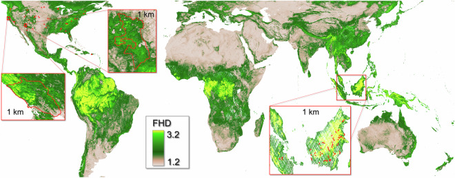
Our overarching goal in creating these near-global canopy structure maps was to increase the accessibility of GEDI data for large extent analyses, with a particular focus on producing high quality-filtered, analysis-ready, gridded vegetation structure metrics. To facilitate these types of analyses, we gridded (i.e. statistically-aggregated) 26 metrics of interest from the GEDI L2A, L2B, and L4A products and 10 additional metrics derived from the L2A and L2B dataset at three spatial resolutions: 1 km, 6 km, and 12 km. We used multiple spatial resolutions in order to provide continuous (i.e. gap-free) coverage for different parts of the world. Furthermore, we gridded structural metrics for each year (2019, 2020, 2021, 2022, and 2023) of the GEDI mission as well as for the full mission (April 2019 to March 2023). Lastly, we quantified uncertainty of mean gridded metrics and the accuracy of canopy height (CH), total PAI, and FHD using independent Airborne Laser Scanning (ALS) surveys (Fig. 1).

Fig. 1.

GEDI mean FHD map using shots from April 2019 to March 2023 at 6 km spatial resolution. Red boxes indicate the approximate location of airborne lidar used for intercomparison. Three insets show GEDI mean FHD at finer spatial resolution (1 km) as well as more detailed airborne lidar coverage (red polygons). From left to right the insets show: Sonoma County, CA, USA, Coconino National Forest, USA, and Sumatra/Borneo.

Methods

Data download

We downloaded all GEDI L2A¹⁵ and L2B¹⁶, as well as GEDI L4A¹⁷ (version 2.1) orbit granule files from April 17 2019 to March 16 2023 to our high performance computing system (HPC). We programmatically downloaded L2 products using a file list obtained from NASA Earthdata search. We used a shell script with the wget utility to automatically download each orbit granule file and verified that the checksum of the downloaded orbit granule file matched the checksum in the associated orbital granule XML file. Checksum verification was an important step considering intermittent connections to the LPDAAC Data Pool. The downloaded L2 data had an approximate volume of 126 Tb. We used the Globus file transfer utility to automatically sync the L4A dataset from the ORNL DAAC to our HPC. The downloaded L4A data had an approximate volume of 14 Tb. A summary of the number of files and data volume is shown in Supplementary Table 1.

Orbital processing and quality filtering

Most processing was done using a combination of R¹⁸ and bash scripts. We used SLURM Workload Manager¹⁹ on our HPC to distribute jobs. We first matched L2A, L2B, and L4A orbit granules using a unique portion of their file names. Then we extracted data from each product granule and converted it to a R data.table²⁰. We only extracted metrics associated with the default ground-finding algorithm (“a0”). The list of metrics selected for gridding is shown in Table 1.

Table 1.

GEDI metrics selected for gridding, their origin, and a brief description.

GEDI metric name	Original GEDI Product Level, Metric Name	Description
agbd-a0, agbd-a0-qf	L4A, agbd	Predicted aboveground biomass density. “-qf” suffix indicated the l4_quality_flag was applied (Mg/ha)
cover-a0	L2B, cover	Total canopy cover, defined as the percent of the ground covered by the vertical projection of canopy material (unitless)
elev-lm-a0	L2A, elev_lowestmode	Elevation of center of lowest mode (ground elevation) relative to WGS84 ellipsoid (meters)
even-pai-1m-a0	Derived from L2B	Evenness of the L2B 1 m vertical Plant Area Index profile (m−1). Calculated as: fhd_normal/log(ceiling(rh100))
even-pavd-5m-a0	Derived from L2B PAVD profile	Evenness of the L2B 5 m vertical Plant Area Volume Density profile (m−1). Calculated as:If (rh-100-a0 > 5) {fhd-pavd-5m-a0/log (number nonzero PAVD bins)}
fhd-pai-1m-a0	L2B, fhd_normal	Foliage height diversity (FHD), or Shannon entropy index, calculated from 1 m vertical bins in the foliage profile, normalized by total plant area (PAI) index (unitless)
fhd-pavd-5m-a0	Derived from L2B PAVD profile	FHD estimated from L2B 5 m plant area volume density (PAVD) vertical profile normalized by total PAVD (unitless)
num-modes-a0	L2A, num_detectedmodes	Number of detected modes in rxwaveform (unitless)
pai-a0	L2B, pai	Total Plant Area Index (PAI; m2/m2)
pavd_0–5-frac	Derived from L2B PAVD profile	The fraction of PAVD in 0 to 5 m height bin relative to the sum of PAVD from all height bins (unitless)
pavd_x-y	L2B, pavd_z	PAVD from x to y m (m2/m3); Height bins are in increments of 5 m, up to 80 m
pavd-bot-frac	Derived from L2B PAVD profile	Fraction of PAVD in the bottom half of the canopy relative to the sum of PAVD from all height bins (unitless). The midpoint is calculated as: (round((rh-100-a0/2)/5)*5)/5
pavd-max-h	Derived from L2B PAVD profile	The upper height of the 5 m bin with maximum PAVD (m)
pavd-top-frac	Derived from L2B PAVD profile	Fraction of PAVD in the top half of the canopy relative to the sum of PAVD from all height bins (unitless). The midpoint is calculated as: (round((rh-100-a0/2)/5)*5)/5
rh-50-a0, rh-95-a0, rh-98-a0	L2A, rh	Relative height (RH) at the 50th, 95th, and 98th percentile of returned energy (m)
rhvdr-b	Derived from L2A rh profile	Bottom canopy vertical distribution ratio (VDR; unitless). Calculated as: If (rh-100-a0 > 5 & rh-50-a0 >  = 0 & rh-98-a0 >  = 0) {rh-50-a0/rh-98-a0}
rhvdr-m	Derived from L2A rh profile	Middle canopy VDR (unitless). Calculated as: If (rh-100-a0 > 5 & rh-25-a0 >  = 0 & rh-75-a0 >  = 0 & rh-98-a0 >  = 0) {(rh-75-a0-rh-25-a0)/rh-98-a0}
rhvdr-t	Derived from L2A rh profile	Top canopy VDR (unitless). Calculated as: If (rh-100-a0 > 5 & rh-50-a0 >  = 0 & rh-98-a0 >  = 0) {(rh-98-a0-rh-50-a0)/rh-98-a0}

We used a quality filtering recipe developed in collaboration with GEDI Science Team members to identify the highest quality GEDI vegetation shots. This recipe closely follows the approach used for the GEDI L4B product. Supplement Section B shows pseudo-code for quality-filtering of each GEDI product. Initial filtering was used to select quality shots that are suitable for ground elevation and vegetation structure metrics. We joined the initial filtered L2A, L2B, and L4A tables together, matching by shot number, longitude of the lowest mode, and latitude of the lowest mode. Then we used a dictionary of local outlier granules produced by University of Maryland to attribute orbit segments (“loc_out_umd”) as having local outliers (1) or not (0). That table is part of the GEDI L4B dataset (gedi_l4b_excluded_granules_v21.json).

Next, we created a L2 high-quality flag (“l2_hqflag”; Supplement B) to distinguish quality shots that are suitable for ground elevation (l2_hqflag == 0 | 1) versus those that are suitable for vegetation metrics (l2_hqflag == 1). To summarize, the L2 high-quality flag signifies the highest geolocation accuracy, that the L2B algorithm was run, surface water percentage is less than 10%, the urban percentage is less than 50%, vegetation is “leaf-on”, no local outliers were detected, PAI and cover values fall within expected ranges, and the absolute elevation difference relative to the TanDEM-X DEM is 150 m or less. We also created a L4A high-quality flag (“l4a_hqflag”; Supplement B) to distinguish high-quality shots that are suitable for aboveground biomass density (l4a_hqflag == 1) versus those that are suitable only for vegetation metrics (l4a_hqflag == 0 | 1). This flag was only used when gridding the metric agbd-a0-qf. Both the l2_hqflag and l4a_hqflag are used for filtering during the gridding procedure (see Supplementary Section B for pseudo-code). Lastly, using the original shot geographic coordinates (lon_lm_a0, lat_lm_a0) we cropped the initial quality-filtered and joined shot tables (attributed with the l2_hqflag and l4a_hqflag flags) associated with each orbit granule to a regular 1 × 1 degree grid (EPSG 4326 geographic coordinates). In other words, the quality shots of each orbit granule were divided into 1 × 1 degree chunks for subsequent distributed processing, resulting in a large number of spatially-indexed tables.

Gridding procedure

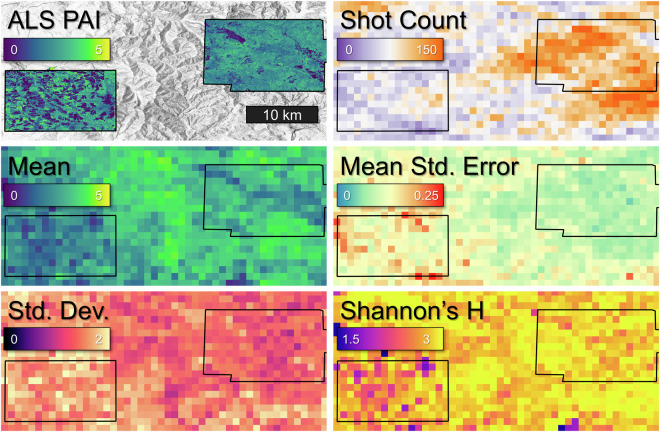
We ran a separate gridding job for each 1 × 1 degree chunk. We first combined all quality shot chunk tables inside of and within a distance of 0.25 degrees of the 1 × 1 degree chunk of interest. Adding a 0.25 degree buffer was necessary to ensure that the edges of the gridded rasters matched (i.e. no edge artifacts in the final mosaic). This resulted in a table which could be used to select a GEDI metric of interest and filter to a specific time period (single year or full mission). At this point we transformed shot geographic coordinates to projected coordinates (EPSG 6933). We ensured that each quality-filtered shot at least had valid values for the fields lon_lm_a0_6933, lat_lm_a0_6933, elev_lm_a0, date_dec, and orbit. We made a distinction between shots suitable for estimating ground elevation versus vegetation structure - we used the field l2_hqflag to identify the highest quality shots to use for gridding vegetation structure metrics. Finally, we looped over each spatial resolution and time period, and gridded each GEDI metric. Prior to the gridding, we used a 30 m raster (EPSG 6933) to select only the first shot (temporally) whose center fell within each 30 m grid cell. This step reduced very dense point clusters which helped to reduce spatial biases in the gridded maps and decreased processing time for mid latitude grids. To compute the gridded values we used the R function terra::rasterize²¹, supplying functions for each aggregation statistic - mean, bootstrapped uncertainty of the mean, median, standard deviation (SD), interquartile range (IQR), Shannon’s Diversity Index, and shot count (Table 2; Fig. 2). We required a minimum of 2 shots per grid cell for gridding to occur, otherwise the pixel was assigned a nodata value (i.e. masked out).

Table 2.

Statistics used for per-pixel aggregation of GEDI shot metrics.

Statistic Band Name Suffix	Description
mean	The mean of GEDI shot metric values within a pixel.
meanbse	Standard error of the mean calculated using bootstrap resampling. We calculated the mean value of GEDI shots for 100 unique bootstrap samples in which we randomly selected 70% of shots. The standard error is calculated using 100 estimates of the mean. Only calculated when there are at least 10 GEDI shots in the grid cell.
med	The median value (50th percentile) of GEDI shot metric values within a pixel.
sd	The standard deviation of GEDI shot metric values within a pixel.
iqr	The interquartile range (75 percentile minus 25th percentile) of GEDI shot metric values within a pixel.
p95	The 95th percentile value of GEDI shot metric values within a pixel.
shan	Shannon’s diversity index (H) of GEDI shot metric values within a pixel. Calculated as:−1*(sum(p*log(p))) where p is the proportion of GEDI shot values per bin. For global map consistency, we used predefined GEDI metric bins (see Supplementary Table 2). Note that at least two bins must be populated, otherwise the returned value is nodata (−9999).
countf	The count of GEDI shot metric values within a pixel. A 30 m sub-grid was used to select the (temporally) first GEDI shot acquired in each 30 m sub-grid cell.

Fig. 2.

NEON ALS Plant Area Index (PAI) at 25 m spatial resolution for the NEON sites ABBY and WREF (Washington state, USA; coverage outlined in black) with USGS 3DEP elevation hillshade as the background. High resolution (1 m) ALS is compared with several GEDI PAI statistical aggregations (shot count, mean, mean standard error, standard deviation, and Shannon’s H) at 1 km resolution from the time period April 17, 2019 to March 16, 2023.

We estimated the uncertainty of the per-pixel mean of each GEDI metric using a bootstrapping approach. For every pixel with at least 10 shots (at each resolution), we took 100 unique random samples of the shots falling within that pixel. For each sample we randomly selected 70% of the available shots (without replacement). We calculated the mean of each unique sample and then calculated the bootstrap standard error of the estimated mean^22,23 using the following bootstrap standard error equation:

$$\mathrm{meanbse}=\sqrt{\frac{{\sum }_{b=1}^B{\left(\mathit{\mu }b-\mathit{\mu }B\right)}^2}{B-1}},$$

where

b corresponds to an individual bootstrap

B is the total number of bootstraps (100 in this case)

μb is the per-pixel mean value of a GEDI metric associated with an individual bootstrap

μB is the per-pixel mean of all individual bootstrap mean, that is ${\sum }_{b=1}^B\frac{\mathit{\mu }b}{B}$

This method is designed to characterize the uncertainty associated with the GEDI sampling strategy, but also incorporates uncertainty associated with variability of topography and vegetation structure within each pixel.

The Shannon Diversity index (H) was computed using a per-pixel histogram of GEDI shot metric values. However, owing to the fact that Shannon’s Diversity index (also known as Shannon’s H) is sensitive to the total number of categories (e.g. vertical bins), for global consistency we defined each metric’s bin width so that the total number of bins used for each metric was relatively equivalent. Specifically, for each metric we identified the range of the bulk (~95%) of the global distribution and divided that number by 20 to determine its bin width. For example, the 95th percentile of the 1 km median total PAI raster is 5.6. Dividing 5.6 by 20 equals 0.28, which we rounded to 0.25. For some metrics we chose a slightly different bin size, informed by our understanding of the metric precision and/or the ecological relevance of a particular value (Supplementary Table 2). For the 98% relative height (RH98) for example, the estimated bin size was 1.8 m, but we increased this to 3 m given the GEDI’s long laser pulse width and potential of some canopies to reach >60 m (which would be ~20 bins). This empirical bin width determination ensures relative cross-compatibility among Shannon diversity values across metrics, while allowing for more than 20 bins (and hence higher Shannon’s values) for those pixels exceeding the maximum of the 95th percentile of the global distribution. In order for the Shannon Diversity Index to be computed, we require that there are at least two bins covered by the GEDI metric values.

We also produced two separate shot count rasters for each spatial resolution and temporal period. These rasters include the total number of shots which are suitable for gridding either all ground elevation (“ga”) or all vegetation metrics (“va”). In both cases, we removed likely outliers using the GEDI L4B excluded granules list. The four bands in the “counts” rasters are described in Supplementary Table 3. They include per-pixel counts of unique shots, orbits, and tracks, as well as the average Nearest Neighbor Index²⁴ (NNI) which is a proxy for quantifying spatial clustering/dispersion of GEDI shots. The NNI is expressed as the ratio of the observed Euclidean distance (m) divided by the expected distance for all shot pairs. The expected distance is the average distance between neighbors in a hypothetical random distribution. If the index is less than 1, the pattern exhibits spatial clustering; if the index is greater than 1, shots are more evenly dispersed.

Each 1 × 1 degree SLURM job produced 123 raster tiles for each temporal period. We used GDAL²⁵ to mosaic these tiles together, resulting in multi-resolution gridded rasters which cover the entire GEDI domain, all longitudes between 52 degrees south and 52 degrees north latitude.

Data Records

The dataset²⁶ is available at Oak Ridge National Laboratory Distributed Active Archive Center (10.3334/ORNLDAAC/2339).

We produced rasters for each GEDI metric listed in Table 1 at three spatial resolutions (1, 6, and 12 km) and over six temporal periods - individual years 2019, 2020, 2021, 2022, 2023, and the full mission (April 17 2019 to March 16 2023). All rasters use a cylindrical, equal-area projection (EPSG:6933) inspired by the Equal-Area Scalable Earth (EASE)-Grid 2.0 Global (https://nsidc.org/data/ease), but with slightly different spatial resolution and extent due to integer pixel dimensions. The rasters are stored as cloud-optimized GeoTiffs (.tif) which have the following characteristics:

• Bands: 8 for GEDI metrics, 4 for counts

• Scale factor: 1

• Layout: COG

• Overview resampling method: nearest

• Tile size (or Block size): 256 by 256

• Compression: LZW

• Map Projection: equal-area cylindrical

• Datum: World Geodetic System 1984

• EPSG: 6933

• NoData Value: −9999

• Resolution specific values listed in Supplementary Table 4

The dataset contains 738 raster files (.tif) totaling 395 GB.

The dataset is also accessible in the Google Earth Engine data catalog. There are three separate image collections corresponding to the three spatial resolutions used for gridding: LARSE/GEDI/GRIDDEDVEG_002/V1/1KM, LARSE/GEDI/GRIDDEDVEG_002/V1/6KM, LARSE/GEDI/GRIDDEDVEG_002/V1/12KM.

Technical Validation

ALS Intercomparison

We used high-resolution gridded ALS to compare select 1 km and 6 km gridded GEDI metrics corresponding to the time period April 17, 2019 to March 16, 2023. We used the following ALS datasets for comparison:

1. National Ecological Observation Network²⁷ (NEON), USA

2. NASA Carbon Monitoring System (CMS) Sonoma County, CA, USA²⁸

3. USGS 3D Elevation Program (3DEP) Coconino National Forest, AZ, USA

4. NASA Carbon Monitoring System (CMS) Indonesia²⁹

5. Ecological and Socioeconomic Functions of Tropical Lowland Rainforest Transformation Systems (EFForTS) Indonesia^30,31

6. Stability of Altered Forest Ecosystem (SAFE) Malaysia³².

For the NEON dataset, we compared canopy height (RH98), height of median energy (RH50), total plant area index (PAI), and foliage height diversity (FHD). For the other five regions we compared canopy height (RH98) at a minimum, and in some cases (when other gridded ALS metrics were already available) we compared additional metrics (Table 3). We report the following statistics for each comparison:

• adjusted R squared (R²) from a linear model of the form ALS~GEDI

• Root mean squared error (RMSE)

• Relative RMSE = 100 * (RMSE/mean(ALS))

• Mean absolute error (MAE)

Table 3.

Summary of ALS datasets used for comparison.

Dataset name	Country, State	ALS Acquisition Dates	ALS pixel size	GEDI Metrics Compared	ALS Data Access
NEON	USA, Multiple States	June-Sept. 2020–2021	1 m	RH98, RH50, PAI, FHD	https://data.neonscience.org/data-products/DP1.30003.001
NASA CMS Sonoma County	USA, California	Sept. 28 - Nov. 26, 2013	3 m	RH98	https://sonomavegmap.org/data-downloads/
USGS 3DEP Coconino	USA, Arizona	Aug. 16 - 20, 2019	1 m	RH98	https://rockyweb.usgs.gov/vdelivery/Datasets/Staged/Elevation/LPC/Projects/AZ_Coconino_2019_B19/AZ_Coconino_B1_2019/
NASA CMS Borneo	Indonesia, Kalimantan	Oct. 18 - Nov. 30, 2014	3 m	RH98	10.3334/ORNLDAAC/1540
EFForTS	Indonesia, Jambi	Jan. 24 - Feb. 5, 2020 and Nov. 21 - 24, 2022	1 m for RH98; 10 m otherwise	RH98, RH50, PAI, FHD	10.25625/CKLY7X, 10.25625/HWTBW5
SAFE	Sabah, Malaysia	Nov. 2014	1 m for RH98; 10 m otherwise	RH98, PAI, FHD	https://zenodo.org/doi/10.5281/zenodo.4020696

NEON

The 1 km gridded GEDI product from the time period April 17, 2019 to March 16, 2023 was compared with NEON ALS data across a large range of latitudes and longitudes throughout the United States. First, we downloaded all ALS point cloud tiles for 31 NEON sites with > 30% forest cover. We queried all ALS tiles between 2020–2021, selecting the year with the best spatial coverage (tiles n), and where tied, selected the most recent year, resulting in approximately 1.5 TB of ALS across all sites. Second, we normalized all point clouds by tile using the lidR package³³ in R. This process entailed instituting a multi-step noise removal algorithm consisting of (a) employing an isolated voxels filter that removes all 1 m voxels filter with fewer than 3 pts/m²; (b) determining the ground surface by estimating a digital terrain model (DTM) by interpolating a convex hull from all points classified as ground and removing all negative values; and (c) normalizing all point heights (z values) by subtracting the DTM from all points, and removing all negative values.

Third, we determined a RH98 canopy height model (CHM) at 1 m spatial resolution as the 98^th percentile of all points/m². Concurrently, we generated PAI and FHD layers at an equivalent resolution of GEDI footprints by estimating plant area density for 25 m pixels using a universal extinction coefficient in the leafR package³⁴ in R. We then calculated FHD as a function of PAI in 1 m vertical height bins. Fourth, we aligned all ALS rasters with corresponding gridded GEDI data by: (a) mosaicking all 1 m RH98 CHMs and 25 m PAI/FHD rasters across each NEON site; (b) masking water and urban classes from each ALS raster based on the 2019 National Land Cover Database³⁵ (NLCD); (c) projecting and resampling all ALS mosaics to match those from gridded GEDI; (d) aggregating 1 m and 25 m rasters to 1 km by mean, median, SD, IQR, 95th percentile, and Shannon’s H; and (e) trimming all edge pixels so that only GEDI and ALS mosaic pixels with 100% overlap (i.e. “core” pixels) were retained. Finally, for comparison, we extracted all co-located ALS and GEDI pixels and assessed accuracy of GEDI relative to ALS. The mean (across all NEON sites) of each comparison statistic is shown in Table 4.

Table 4.

The mean (across all NEON sites) of each comparison statistic (RMSE, Rel. RMSE, MAE, and Adj. R²) for each GEDI metric and aggregation statistic at 1 km spatial resolution.

GEDI metric	Aggregation Statistic	RMSE (m)	Rel. RMSE (%)	MAE (m)	Adj. R2	N 1 km2 samples
RH98	Mean	3.35	24	2.43	0.91	3515
RH98	Median	3.88	28	2.69	0.89	3515
RH98	SD	2.21	45	1.51	0.69	3515
RH98	IQR	4.06	60	2.70	0.61	3515
RH98	95th Perc.	5.03	23	3.07	0.87	3515
RH98	Shannon’s H	0.39	26	0.29	0.68	3515
RH50	Mean	2.43	43	1.62	0.90	3515
RH50	Median	2.90	54	1.77	0.88	3515
RH50	SD	1.57	51	1.12	0.73	3515
RH50	IQR	3.12	75	2.03	0.60	3515
RH50	95th Perc.	3.92	36	2.66	0.85	3515
RH50	Shannon’s H	0.59	42	0.44	0.67	3493
PAI	Mean	0.59	57	0.40	0.82	3515
PAI	Median	0.66	65	0.43	0.79	3515
PAI	SD	0.67	157	0.53	0.33	3515
PAI	IQR	0.93	160	0.63	0.30	3515
PAI	95th Perc.	1.65	94	1.25	0.57	3515
PAI	Shannon’s H	0.64	43	0.50	0.53	3515
FHD	Mean	0.56	29	0.42	0.88	3515
FHD	Median	0.64	33	0.45	0.85	3515
FHD	SD	0.23	45	0.17	0.46	3515
FHD	IQR	0.48	71	0.30	0.40	3515
FHD	95th Perc.	0.48	18	0.32	0.83	3515
FHD	Shannon’s H	0.57	23	0.40	0.19	3515

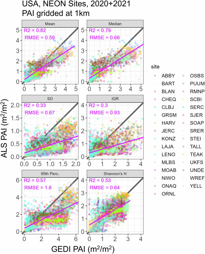
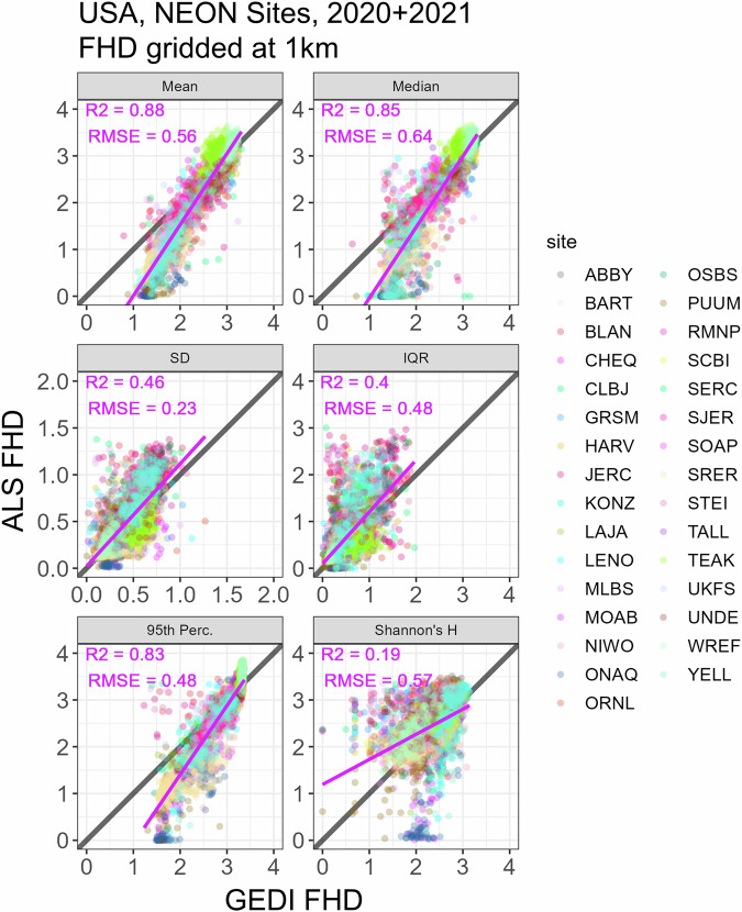
Below (Figs. 3–4) we show comparison plots for GEDI PAI and FHD gridded at 1 km spatial resolution using the statistics mean, median, SD, IQR, 95th Percentile, and Shannon’s H. Additional NEON comparison plots and tables (RH98 and RH50) are shown in Supplementary Section D. Given the extents of the individual NEON sites and ALS surveys we did not perform comparisons at spatial resolutions coarser than 1 km.

Fig. 3.

Comparison of NEON ALS PAI and GEDI PAI using mean, median, SD, IQR, 95th percentile, and Shannon’s H aggregation methods from the time period April 17, 2019 to March 16, 2023. The black line has a 1:1 relationship while the purple line corresponds to a linear fit (ALS~GEDI) of 1 km cells from all NEON sites.

Fig. 4.

Comparison of NEON ALS FHD and GEDI FHD using mean, median, SD, IQR, 95th percentile, and Shannon’s H aggregation methods from the time period April 17, 2019 to March 16, 2023. The black line has a 1:1 relationship while the purple line corresponds to a linear fit (ALS~GEDI) of 1 km cells from all NEON sites.

Additional ALS

We made use of other readily available ALS datasets in the USA and Southeast Asia for additional comparisons. Fine resolution canopy height models, and in some cases other gridded metrics, were distributed with some ALS datasets, specifically NASA CMS Borneo, EFForTS, and SAFE (Table 3). These metrics were computed with commonly used packages like lidR³³, leafR³⁴, and PDAL^36,37. For USGS 3DEP Coconino we computed a high spatial resolution canopy height model by subtracting a digital surface model from a digital terrain model, both computed using PDAL. We uploaded the high-resolution ALS rasters along with associated gridded GEDI rasters from the time period April 17, 2019 to March 16, 2023 to Google Earth Engine³⁸ where we developed a comparison script.

Similar to the steps described for NEON comparison, we used a combination of masks to ensure a fair comparison between ALS and GEDI at spatial resolutions greater than or equal to 1 km. First we identified heavily urban or surface water pixels since these areas are not relevant for comparison. For the USA, we used NLCD 2021 land cover to determine urban and surface water pixels. For Southeast Asia, we used the mean GLAD annual surface water percentage³⁹ and urban classification from Copernicus Global Land Service 100 m Land Cover to define water and urban masks⁴⁰. Furthermore, considering the forest structure dynamics (especially in Southeast Asia) we added a mask to identify pixels which had undergone a stand-replacing disturbance⁴¹ during the year of or after the primary ALS acquisition year. We combined these three masks together to summarize the valid percent of each gridded pixel (i.e. not surface water, not urban, and not disturbed). In order for a gridded pixel to be eligible for comparison we required that at least 90% of the 30 m pixels used to determine the combined mask be valid. We extracted the corresponding ALS and GEDI gridded values for each metric, aggregation statistic, and pixel. We exported the resulting table to R and produced scatter plots and summary statistic tables.

ALS data were acquired for Sonoma County, CA, USA in 2013. We used a 3 m spatial resolution canopy height model for comparison. Given the large extent of the County, we performed the comparison at 1 km (Fig. 5) and 6 km spatial resolution. Additional comparison plots and tables are shown in Supplementary Section D. Note that there is at least 6 years between ALS and GEDI lidar acquisition, so some error may be attributable to growth and/or non-stand-replacing disturbances.

Fig. 5.

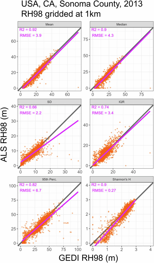
Comparison of Sonoma County ALS RH98 and GEDI RH98 using mean, median, SD, IQR, 95th percentile, and Shannon’s H aggregation methods from the time period April 17, 2019 to March 16, 2023. The black line has a 1:1 relationship while the purple line corresponds to a linear fit (ALS~GEDI) of 1 km cells.

ALS data were acquired for Coconino National Forest, AZ, USA (and some surrounding areas) in 2019. We computed a 1 m spatial resolution canopy height model for comparison. Given the large extent of the National Forest, we performed the comparison at 1 km (Fig. 6) and 6 km spatial resolution. Additional comparison plots and tables are shown in Supplementary Section D.

Fig. 6.

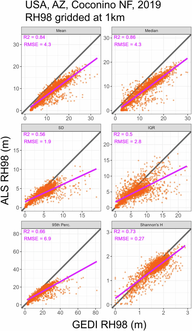
Comparison of Coconino National Forest ALS RH98 and GEDI RH98 using mean, median, SD, IQR, 95th percentile, and Shannon’s H aggregation methods from the time period April 17, 2019 to March 16, 2023. The black line has a 1:1 relationship while the purple line corresponds to a linear fit (ALS~GEDI) of 1 km cells.

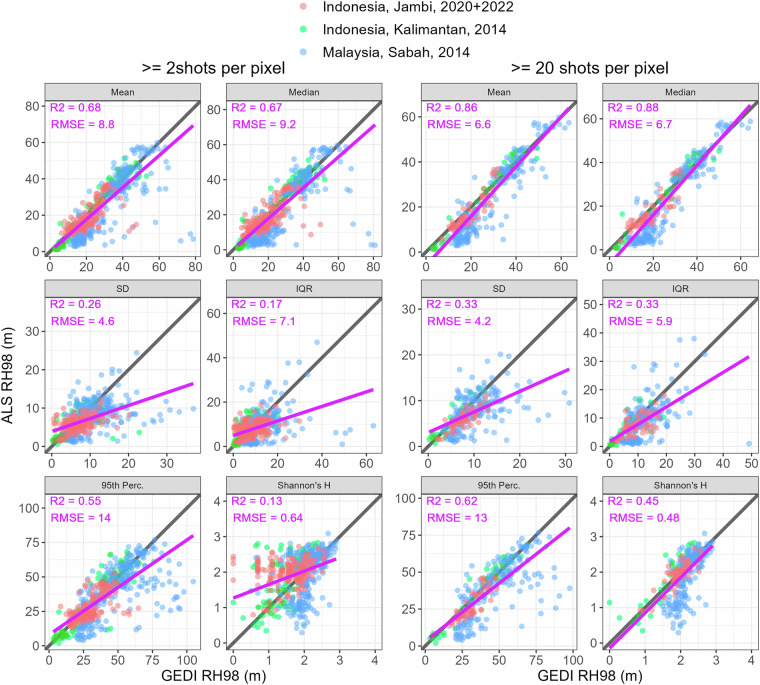
In addition to these temperate sites, we downloaded publicly available tropical forest ALS data associated with three projects in Southeast Asia, namely NASA CMS Borneo, EFForTS, and SAFE. As part of the NASA CMS Borneo project, ALS data were acquired for select regions of Kalimantan, Indonesia in 2014. We used a 3 m spatial resolution canopy height model for comparison. ALS data were acquired for the SAFE project landscape, Maliau Conservation Area and Danum Valley of Sabah, Malaysia in 2014. We used a 1 m spatial resolution canopy height model for comparison. We also used 20 m gridded maps of total PAI and FHD for comparison and present those results in Supplementary Section D. As part of the EFForTS project, ALS data were acquired for select regions of Jambi, Indonesia in 2020 and 2022. We mosaiced the 1 m canopy height models from the two years, giving priority to the data from 2020 since it covered more area. Rasters of additional ALS metrics (ZQ50, LAI, and FHD) were also available at 10 m spatial resolution. These additional ALS metrics were computed using slightly different equations relative to GEDI, but are still useful for preliminary comparison of gridded GEDI RH50, PAI, and FHD. We show comparison results for RH50, PAI, and FHD in Supplementary Section D. Given the relatively small collection extents of the three campaigns we only performed comparisons at 1 km spatial resolution. For the NASA CMS Borneo and SAFE projects there is at least 5 years between ALS and GEDI lidar acquisition, so some error may be attributable to growth and/or non-stand-replacing disturbances. Figure 7 shows comparison results for RH98 considering all three Southeast Asia projects, highlighting the impact of applying a higher per-pixel shot threshold. Supplementary Section D also includes comparison results for RH98, RH50, PAI, and FHD by individual project.

Fig. 7.

Comparison of SE Asia ALS RH98 and GEDI RH98 using mean, median, SD, IQR, 95th percentile, and Shannon’s H aggregation methods from the time period April 17, 2019 to March 16, 2023. The black line has a 1:1 relationship while the purple line corresponds to a linear fit (ALS~GEDI) of 1 km cells. The left set of plots use a minimum of 2 shots per pixel while the right set of plots only use pixels which have at least 20 shots.

Usage Notes

Considering that this is a product with near-global extent, the uncertainty and comparative assessments with ALS should be viewed as a work in progress and are not comprehensive. Through our comparative assessments thus far we have learned that the gridding procedure generally works well in regions with relatively high GEDI shot density and low to moderate topography (i.e. slope and roughness), like the NEON sites in the USA. The mean, median, and 95th percentile aggregation statistics show the best fit relative to corresponding gridded ALS. The SD, IQR, and Shannon’s H statistics generally have poorer fits and higher relative errors. These results suggest that GEDI generally captures the central and maximum tendencies of various vegetation structure metrics at multiple spatial resolutions, but does not always capture (horizontal) variability as well. The latter result is not necessarily surprising considering GEDI’s sparse sampling density.

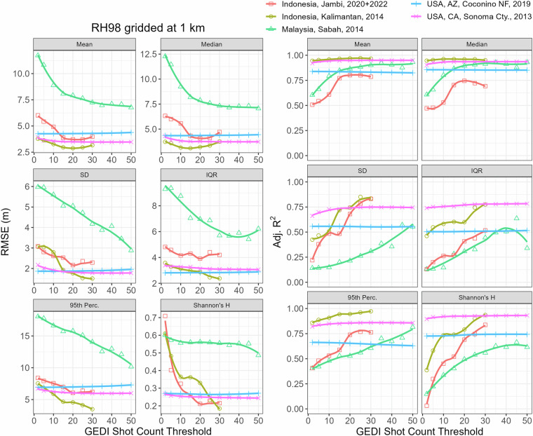
Users should be cautious when using this product in areas with very low shot densities, like some parts of the tropics. ALS comparisons in Indonesia and Malaysia showed mixed results when using a minimum of two GEDI shots per grid cell (Fig. 7). RH98 compared well to ALS in Kalimantan, Indonesia, but relatively poorly in Jambi, Indonesia and Sabah, Malaysia. The poor comparisons in this region are likely the result of a combination of factors, including low shot density, erroneous GEDI measurements associated with clouds, and/or the forest dynamics in the region. Work is ongoing to better estimate shot density thresholds that result in relatively accurate gridded estimates, but here we highlight the impact of the minimum number of shots per grid cell on gridded GEDI metric accuracy in Fig. 8. RMSE decreases and model fit improves as the minimum number of shots per grid cell is increased. For the mean and median statistics, RMSE and R² tend to level off near a threshold of 20 shots per cell. Although, the tradeoff of increasing the minimum number of shots per grid is that fewer grid cells will be available for analysis (i.e. there will be more gaps). Users may also find it beneficial to explore per-pixel filters using the associated “counts_va” rasters which include the number of unique tracks and orbits per pixel. Requiring more than 1 orbit per pixel decreases the likelihood of errors associated with ground-finding and/or inclusion of low clouds in the returned waveform.

Fig. 8.

Comparison of all ALS RH98 RMSE and Adj. R² as a function of GEDI shot count threshold. We required at least 20 pixels for a given shot count threshold to compute RMSE and Adj. R².

Users should also be aware that topography influences many GEDI metrics and this may produce artifacts in some gridded GEDI metrics. The GEDI laser pulse width is relatively long (~15 ns) and the RH profile associated with the returned waveform may be further elongated on steep slopes or rough terrain, even if the area has little to no vegetation. An example of this topographic effect can be seen in the Grand Canyon of Arizona, USA where vegetation within the Canyon is generally low stature, yet 1 km gridded mean RH98 (an estimate of canopy height) frequently exceeds 10 m (Supplementary Figure 13).

Finally, users may notice unexpected gaps in the mid latitudes, especially in 1 km resolution gridded rasters. Globally, most gaps are associated with ISS orbital geometry and cloud cover patterns, but there are some surprising gaps associated with vegetation phenology. Given that our primary goal was to produce gridded maps of vegetation structure metrics, we used “leaf-on” GEDI shots. The exact timing of “leaf-on” vs “leaf-off” was estimated using a VIIRS/NPP data product (VNP22Q2) which has its own uncertainties and limitations. Hence, some large regions containing a large fraction of deciduous vegetation have less gridded coverage relative to pixels at similar latitudes owing to the large number of leaf-off shots that we filtered out. Examples where gridded coverage is limited due to phenology include the Eastern USA and Sierra Madre Occidental, Mexico (Supplementary Figure 14).

Author contributions

P.B., C.H. and S.G. conceptualized the data product and wrote the manuscript. P.B. performed data processing. P.B. and C.H. performed ALS intercomparison.

Code availability

The code is publicly accessible on Github: https://github.com/burnspat/gedi_gridding.

Competing interests

The authors declare no competing interests.

Supplementary information

The online version contains supplementary material available at 10.1038/s41597-024-03668-4.

References

- 1.Deere, N. J. et al. Maximizing the value of forest restoration for tropical mammals by detecting three-dimensional habitat associations. Proceedings of the National Academy of Sciences117, 26254–26262 (2020). 10.1073/pnas.2001823117 [DOI] [PMC free article] [PubMed] [Google Scholar]
- 2.Davis, F. W. et al. LiDAR-derived topography and forest structure predict fine-scale variation in daily surface temperatures in oak savanna and conifer forest landscapes. Agricultural and Forest Meteorology269–270, 192–202 (2019). 10.1016/j.agrformet.2019.02.015 [DOI] [Google Scholar]
- 3.Hakkenberg, C. R. et al. Inferring alpha, beta, and gamma plant diversity across biomes with GEDI spaceborne lidar. Environ. Res.: Ecology2, 035005 (2023). [Google Scholar]
- 4.Pfeifer, M., Disney, M., Quaife, T. & Marchant, R. Terrestrial ecosystems from space: a review of earth observation products for macroecology applications. Global Ecology and Biogeography21, 603–624 (2012). 10.1111/j.1466-8238.2011.00712.x [DOI] [Google Scholar]
- 5.Gouveia, S. F. et al. Forest structure drives global diversity of primates. J Anim Ecol83, 1523–1530 (2014). 10.1111/1365-2656.12241 [DOI] [PubMed] [Google Scholar]
- 6.Oliveira, B. F. & Scheffers, B. R. Vertical stratification influences global patterns of biodiversity. Ecography42, 249–249 (2019). 10.1111/ecog.03636 [DOI] [Google Scholar]
- 7.Pillay, R. et al. Humid tropical vertebrates are at lower risk of extinction and population decline in forests with higher structural integrity. Nat Ecol Evol6, 1840–1849 (2022). 10.1038/s41559-022-01915-8 [DOI] [PubMed] [Google Scholar]
- 8.Dubayah, R. et al. The Global Ecosystem Dynamics Investigation: High-resolution laser ranging of the Earth’s forests and topography. Science of Remote Sensing1, 100002 (2020). 10.1016/j.srs.2020.100002 [DOI] [Google Scholar]
- 9.Dubayah, R. et al. GEDI L1B Geolocated Waveform Data Global Footprint Level V002.10.5067/GEDI/GEDI01_B.002 (2021). 10.5067/GEDI/GEDI01_B.002 [DOI] [Google Scholar]
- 10.Dubayah, R. O. et al. Global Ecosystem Dynamics Investigation (GEDI) GEDI L3 Gridded Land Surface Metrics, Version 2. 0 MB10.3334/ORNLDAAC/1952 (2021). 10.3334/ORNLDAAC/1952 [DOI] [Google Scholar]
- 11.Dubayah, R. O. et al. Global Ecosystem Dynamics Investigation (GEDI) GEDI L4B Gridded Aboveground Biomass Density, Version 2.10.3334/ORNLDAAC/2017 (2022). 10.3334/ORNLDAAC/2017 [DOI] [Google Scholar]
- 12.Potapov, P. et al. Mapping global forest canopy height through integration of GEDI and Landsat data. Remote Sensing of Environment253, 112165 (2021). 10.1016/j.rse.2020.112165 [DOI] [Google Scholar]
- 13.Lang, N., Jetz, W., Schindler, K. & Wegner, J. D. A high-resolution canopy height model of the Earth. Nat Ecol Evol7, 1778–1789 (2023). 10.1038/s41559-023-02206-6 [DOI] [PMC free article] [PubMed] [Google Scholar]
- 14.Mutanga, O., Masenyama, A. & Sibanda, M. Spectral saturation in the remote sensing of high-density vegetation traits: A systematic review of progress, challenges, and prospects. ISPRS Journal of Photogrammetry and Remote Sensing198, 297–309 (2023). 10.1016/j.isprsjprs.2023.03.010 [DOI] [Google Scholar]
- 15.Dubayah, R. et al. GEDI L2A Elevation and Height Metrics Data Global Footprint Level V002.10.5067/GEDI/GEDI02_A.002 (2021). 10.5067/GEDI/GEDI02_A.002 [DOI] [Google Scholar]
- 16.Dubayah, R. et al. GEDI L2B Canopy Cover and Vertical Profile Metrics Data Global Footprint Level V002.10.5067/GEDI/GEDI02_B.002 (2021). 10.5067/GEDI/GEDI02_B.002 [DOI] [Google Scholar]
- 17.Dubayah, R. O. et al. GEDI L4A Footprint Level Aboveground Biomass Density, Version 2.1. ORNL DAAC10.3334/ORNLDAAC/2056 (2022). 10.3334/ORNLDAAC/2056 [DOI] [Google Scholar]
- 18.R Core Team. R: A Language and Environment for Statistical Computing. (R Foundation for Statistical Computing, Vienna, Austria, 2021).
- 19.Jette, M. A. & Wickberg, T. Architecture of the Slurm Workload Manager. in Job Scheduling Strategies for Parallel Processing (eds. Klusáček, D., Corbalán, J. & Rodrigo, G. P.) 3–23. 10.1007/978-3-031-43943-8_1 (Springer Nature Switzerland, Cham, 2023).
- 20.Dowle, M. & Srinivasan, A. Data.Table: Extension of ‘data.Frame’. (2023).
- 21.Hijmans, R. J. Terra: Spatial Data Analysis. (2023).
- 22.Efron, B. & Tibshirani, R. J. An Introduction to the Bootstrap. 10.1201/9780429246593 (Chapman and Hall/CRC, New York, 1994).
- 23.McRoberts, R. E. et al. How many bootstrap replications are necessary for estimating remote sensing-assisted, model-based standard errors? Remote Sensing of Environment288, 113455 (2023). 10.1016/j.rse.2023.113455 [DOI] [Google Scholar]
- 24.Evans, J. S. & Murphy, M.A. spatialEco. R package version 2.0-2, https://github.com/jeffreyevans/spatialEco (2023).
- 25.GDAL/OGR contributors. GDAL/OGR Geospatial Data Abstraction Software Library. 10.5281/zenodo.5884351 (Open Source Geospatial Foundation, 2024).
- 26.Burns, P., Hakkenberg, C., Goetz, S. Gridded GEDI Vegetation Structure Metrics and Biomass Density at Multiple Resolutions. ORNL DAAC10.3334/ORNLDAAC/2339 (2024).
- 27.National Ecological Observatory Network (NEON). Discrete return LiDAR point cloud (DP1.30003.001): RELEASE-2024. 9.5 TB. 10.48443/HJ77-KF64 (2024).
- 28.Dubayah, R. O. et al. CMS: LiDAR-derived Biomass, Canopy Height and Cover, Sonoma County, California, 2013. 45.774511000000004 MB 10.3334/ORNLDAAC/1523 (2017).
- 29.Melendy, L. et al. CMS: LiDAR-derived Canopy Height, Elevation for Sites in Kalimantan, Indonesia, 2014. ORNL DAAC10.3334/ORNLDAAC/1540 (2017). 10.3334/ORNLDAAC/1540 [DOI]
- 30.Camarretta, N., Knohl, A., Erasmi, S. & Schlund, M. Rasters for ALS metrics at 10m resolution. GRO.data10.25625/HWTBW5 (2023). 10.25625/HWTBW5 [DOI] [Google Scholar]
- 31.Camarretta, N. & Schlund, M. Canopy Height Models. GRO.data10.25625/CKLY7X (2021). 10.25625/CKLY7X [DOI] [Google Scholar]
- 32.Swinfield, T., Milodowski, D., Jucker, T., Michele, D. & Coomes, D. LiDAR canopy structure 2014. Zenodo10.5281/zenodo.4020697 (2020). 10.5281/zenodo.4020697 [DOI]
- 33.Roussel, J.-R. et al. lidR: An R package for analysis of Airborne Laser Scanning (ALS) data. Remote Sensing of Environment251, 112061 (2020). 10.1016/j.rse.2020.112061 [DOI] [Google Scholar]
- 34.Almeida, D. R. A. de, Stark, S. C., Silva, C. A., Hamamura, C. & Valbuena, R. leafR: Calculates the Leaf Area Index (LAD) and Other Related Functions. (2021).
- 35.Dewitz, J. National Land Cover Database (NLCD) 2019 Products (ver. 3.0, February 2024). 10.5066/P9KZCM54 (2024).
- 36.PDAL contributors. PDAL: The Point Data Abstraction Library.10.5281/zenodo.2616780 (2022). 10.5281/zenodo.2616780 [DOI] [Google Scholar]
- 37.Butler, H. et al. PDAL/PDAL: 2.6.3.10.5281/ZENODO.2616780 (2024). 10.5281/ZENODO.2616780 [DOI] [Google Scholar]
- 38.Gorelick, N. et al. Google Earth Engine: Planetary-scale geospatial analysis for everyone. Remote Sensing of Environment202, 18–27 (2017). 10.1016/j.rse.2017.06.031 [DOI] [Google Scholar]
- 39.Pickens, A. H. et al. Global seasonal dynamics of inland open water and ice. Remote Sensing of Environment272, 112963 (2022). 10.1016/j.rse.2022.112963 [DOI] [Google Scholar]
- 40.Buchhorn, M. et al. Copernicus Global Land Service: Land Cover 100m: collection 3: epoch 2019: Globe. Zenodo10.5281/zenodo.3939050 (2020). 10.5281/zenodo.3939050 [DOI]
- 41.Hansen, M. C. et al. High-Resolution Global Maps of 21st-Century Forest Cover Change. Science342, 850–853 (2013). 10.1126/science.1244693 [DOI] [PubMed] [Google Scholar]
Associated Data
This section collects any data citations, data availability statements, or supplementary materials included in this article.
Data Citations
- Melendy, L. et al. CMS: LiDAR-derived Canopy Height, Elevation for Sites in Kalimantan, Indonesia, 2014. ORNL DAAC10.3334/ORNLDAAC/1540 (2017). 10.3334/ORNLDAAC/1540 [DOI]
- Swinfield, T., Milodowski, D., Jucker, T., Michele, D. & Coomes, D. LiDAR canopy structure 2014. Zenodo10.5281/zenodo.4020697 (2020). 10.5281/zenodo.4020697 [DOI]
- Buchhorn, M. et al. Copernicus Global Land Service: Land Cover 100m: collection 3: epoch 2019: Globe. Zenodo10.5281/zenodo.3939050 (2020). 10.5281/zenodo.3939050 [DOI]
Supplementary Materials
Data Availability Statement