A novel Bayesian generative approach for estimating tumor dynamics from published studies

Abstract

Tumor growth inhibition (TGI) modeling attempts to describe the time course changes in tumor size for patients undergoing cancer therapy. TGI models present several advantages over traditional exposure–response models that are based explicitly on clinical end points and have become a popular tool in the pharmacometrics community. Unfortunately, the data required to fit TGI models, namely longitudinal tumor measurements, are sparse or often not available in literature or publicly accessible databases. On the contrary, common end points such as progression‐free survival (PFS) and objective response rate (ORR) are directly derived from longitudinal tumor measurements and are routinely published. To this end, a Bayesian generative model relating underlying tumor dynamics to summary PFS and ORR data is introduced to learn TGI model parameters using only published summary data. The parameterized model can describe the tumor dynamics, quantify treatment effect, and account for differences in the study population. The utility of this model is shown by applying it to several published studies, and learned parameters are combined to simulate an in silico trial of a novel combination therapy in a novel setting.

Study Highlights.

• WHAT IS THE CURRENT KNOWLEDGE ON THE TOPIC?

TGI models require individual longitudinal tumor measurements to fit which typically are not made publicly available. No methodology currently exists for fitting TGI models to general studies using published PFS and ORR data in a comprehensive way.

• WHAT QUESTION DID THIS STUDY ADDRESS?

How can published summary‐level data such as PFS and ORR for general studies be used to learn the parameters of a TGI model?

• WHAT DOES THIS STUDY ADD TO OUR KNOWLEDGE?

A Bayesian generative model is introduced that relates the full generative process of published PFS and ORR data from latent tumor dynamics, allowing estimation of the latter using only the former. The model comprehensively captures important details of this process such as nontarget progression and tumor size requirements for progression. The utility of the model in simulating novel clinical trials in silico without individual longitudinal tumor measurements is showcased.

• HOW MIGHT THIS CHANGE DRUG DISCOVERY, DEVELOPMENT, AND/OR THERAPEUTICS?

The model allows for the extraction of TGI model parameters using only publicly available information. Such information can be used in several ways to hasten early decision time and cut costs using in silico trials. For example, TGI parameters learned from published data can be used to better power early studies where little data are available or generalize existing data to a new regime such as an earlier line of therapy. Additionally, TGI model parameters of existing therapies learned from published studies can be used to simulate early phase I assets head‐to‐head and in combination with existing therapies, thus giving an early idea of the feasibility of such assets without the costs and wait time of a full in vivo trial.

INTRODUCTION

Tumor growth inhibition (TGI) modeling attempts to describe the intrinsic dynamics of tumor growth in cancer patients and incorporate the effect of treatment. Unlike univariate exposure–response analyses which consider some marker at a snapshot in time, TGI models are fit on longitudinal measurements of the sum of longest diameters (SLD) of lesions which are typically measured using CT every couple of months. TGI modeling has gained popularity in the pharmacometrics community because of its advantages over univariate exposure–response analyses. ¹ , ² First, TGI modeling can capture the effect on response that may happen when drug exposure varies significantly over time. This often occurs in practice when patients have, for example, dose reductions, varied dosing regimens, or exposure‐lowering anti‐drug antibodies. Second, because the entire longitudinal history of SLD is being modeled, multiple quantities of interest such as the maximum reduction, the time to maximum reduction, or the doubling time can all be captured by a single unified model. When nontarget progression is incorporated in a TGI model as time‐to‐event data modeled by a hazard function as in ³ and more recently, ⁴ this can be taken a step further and common end points such PFS and ORR can be predicted by using a TGI model as well. Third, TGI modeling is a flexible framework; it can incorporate the biological knowledge on the mechanism of action of the drug, and hence the parameters of a TGI model often have mechanistic interpretations. The semi‐mechanistic nature of a TGI framework hence allows natural extensions to make predictions for various scenarios of interest, such as combination therapy. ⁴ , ⁵

TGI models present several upsides to pharmacometricians, but one of their major difficulties in practice is that these models require a somewhat rich set of longitudinal SLD data to fit. As such data are not often publicly available or only span at most a few treatments in a few indications, the utility of TGI models may be limited in clinical development.

While individual SLD data are rarely publicly available, end points such as PFS and ORR are routinely published. PFS and ORR are summary statistics derived directly from longitudinal SLD data by applying a specific set of rules specified by the RECIST criteria. ⁶ Specifically, progression occurs either by target or by nontarget progression. Target progression occurs the first time an SLD measurement is at least 20% and 5 mm larger than the smallest SLD observed thus far. Nontarget progression occurs either when nontarget lesions progress, new lesions appear, or the patient dies. Similarly, response is determined from SLD data and occurs when an SLD measurement is at least 30% smaller than baseline.

PFS and ORR thus embed information about longitudinal SLD data. Thus, in principle, by reversing the RECIST rules, it should be possible to utilize PFS and ORR to infer the possible set of trajectories of SLD and ultimately the parameters of a TGI model. To that extent, the authors of ⁷ created a novel statistical approach for extracting tumor growth rates from published PFS curves and risk tables. Their approach utilized the fact that published PFS curves and risk tables are informative as to the specific progression times in a study and the number of individual progressions occurring at each of those times. They took those progression times and transformed them to an individual growth rate, $k_g$, by assuming exponential growth of SLD and approximating the progression time as simply the first time SLD was at least 20% larger than its initial size. These individual growth rate estimates were then used to estimate population‐level parameters describing the inter‐individual variation of $k_g$ in the study population using a two‐step procedure. The key limitation of this approach is the assumption of exponential growth, which often is true only for studies where the growth can be described by a single parameter exponential function, typically for studies with small to negligible drug effect. Therefore, the authors were limited to only considering “failed” studies where treatment effects were small and thus effective growth rates, $k_{\mathrm{eff}}=k_g-k_{\text{kkill}}$, were close to baseline growth rates, $k_g$. Furthermore, certain aspects of clinically deemed tumor progression were ignored; for example, that progression need not occur from an increase in SLD, but may also occur due to nontarget progression, or that absolute tumor size needs to be modeled because the criteria for progression also stipulates an increase of at least 5 mm. Furthermore, this approach does not utilize other typically published information that is informative of underlying tumor dynamics such as ORR which can make the inference more robust.

Extending the approach of ⁷ for backwards estimation of growth dynamics from PFS data and relaxing these assumptions in the setting of deterministic estimators is difficult. On the contrary, a probabilistic forward process, by which a study population with TGI dynamics and SLD measurements are all sampled to generate PFS and ORR data may be easily feasible. By specifying this data‐generating process in terms of a set of conditional distributions, Bayes' rule can then be applied to solve the backward inference problem, which provides a framework to overcome the key limitations of the assumptions.

More generally, Bayesian generative models, or probabilistic graphical models, provide a flexible and general framework for modeling how a set of observed data may have arisen from a set of underlying causes. Such models are often represented by probabilistic diagrams that encode the joint probability distribution between unobserved variables and observed data and are used commonly in the Bayesian statistics and machine learning literature. ⁸ , ⁹ This joint distribution can be subsequently used to infer causal relationships and parameters of interest by conditioning on observed data and applying Bayes' rule. Probabilistic programming languages such as BUGS, JAGS, Stan, PyMC3, Turing, and Pyro ¹⁰ , ¹¹ , ¹² , ¹³ , ¹⁴ , ¹⁵ have gained popularity because their ease‐of‐use and ability to infer general probabilistic models by simply specifying this joint distribution. Indeed, these modeling frameworks have been increasingly used in pharmacometrics because of their ability to easily describe and infer complex models. ¹⁶ , ¹⁷ , ¹⁸

To that end, this work introduces a novel approach using Bayesian generative modeling for estimating tumor dynamics from summary‐level clinical datasets containing only information on PFS and ORR. In the following sections, we first present an overview of the data‐generating model and joint distribution of parameters, latent variables, and observed data. Next, the inference procedure and details are described. We illustrate the validity of the approach by presenting the model's ability to recover underlying tumor dynamics from simulated data when the ground truth is known. Finally, we showcase the utility of the framework by characterizing the tumor dynamics from three published studies in metastatic castration‐resistant prostate cancer (mCRPC), and we use these learned dynamics to build a tumor dynamics model to simulate in silico trials of existing drugs in new patient settings and treatment regimes, including combination therapy.

METHODS

Bayesian generative model of published PFS and ORR data

A Bayesian generative model was developed specifying the joint distribution of trial‐specific parameters, arm‐specific parameters, individual patient parameters, individual SLD observations, nontarget progression, and reported PFS and ORR in a published study. The model is summarized in Figure 1a. The model includes a semi‐mechanistic population TGI component to capture measured longitudinal tumor dynamics at the individual and population level. However, unlike a standard population TGI model which relates tumor dynamics to observed longitudinal measurements, the model includes extra components that further relate these longitudinal measurements to downstream PFS and response based on the RECIST criteria. Crucially, the specification of this joint distribution allows for joint estimation of all model parameters conditioned on observed summary data using standard Bayesian estimation.

FIGURE 1.

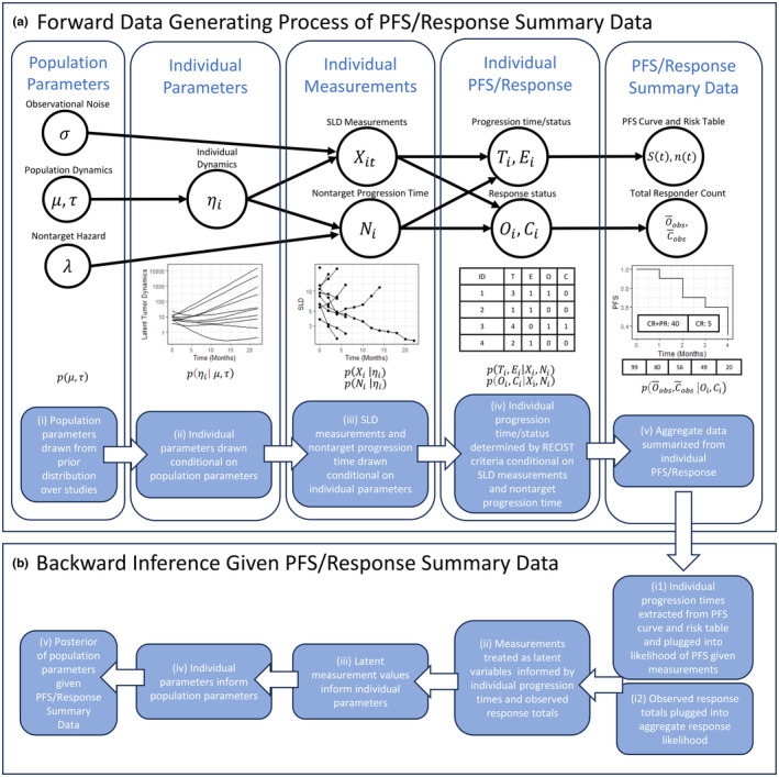
(a) Entire data‐generative process of population tumor growth inhibition (TGI) model and summary progression‐free survival (PFS)/response data as a probabilistic graphical model. (ai) First, population parameters μ and $\tau$ are drawn from a prior distribution of study populations. (aii) Conditional on these values, individual parameters are drawn for each patient in the study, parameterizing their individual latent dynamics. (aiii) Conditional on these individual dynamics, sum of longest diameters (SLD) measurements and a nontarget progression time, $X$ and $N$ respectively, are drawn for each patient. (aiv) Conditional on those values, progression or dropout time, $T$, dropout status, $E$, response status, $O$, and complete response status, $C$, are determined simply following RECIST rules. (av) Finally from these, the commonly published summary PFS curve and ORR are determined. (b) Overview of backward inference of TGI model parameters starting from PFS/response summary data. (bi1) Individual progression times/statuses are extracted and plugged in to individual likelihoods. (bi2) Observed response totals are plugged in to the aggregate response likelihood. (bii) Measurements are treated as latent variables and informed by these likelihoods. (biii–v) The individual measurements go on to inform the individual parameters which inform the population parameters through the conditional distributions.

Although the method is not restricted to any particular form of the underlying mechanistic model of tumor dynamics, in the examples herein individual tumor dynamics were described using a standard biexponential model:

$$R\left(t\right)=R_0\left[{\mathit{fe}}^{\left(k_g-k_{\mathit{\text{kkill}}}\right)t}+\left(1-f\right)e^{\left(k_g-k_{\mathit{\text{kkillr}}}\right)t}\right]$$

with parameters $R_0$ representing the initial SLD in millimeters, $k_g$ the baseline growth rate per day, $k_{\mathit{\text{kkillr}}}<k_{\mathit{\text{kkill}}}$ the drug‐induced killing rates per day for normal and more resistant cells respectively, and $f$ the initial proportion of normal versus more resistant cells.

$R_0$, $k_g$, and $f$ are individual‐specific and drawn conditional on population parameters $\mu$ and $\tau$ for each of the three respective parameters (Figure 1aii). $k_{\mathit{\text{kkill}}}$ and $k_{\mathit{\text{kkillr}}}$ are not modeled as patient‐specific and are determined by the arm of a study that a patient belongs to in a multi‐arm study. For brevity, ${\eta }_i$ denotes the vector ($R_0^{\left(\mathrm{i}\right)}$, $k_g^{\left(\mathrm{i}\right)}$, $f^{\left(\mathrm{i}\right)},k_{\mathit{\text{kkill}}}$, $k_{\mathit{\text{kkillr}}}$). Details of the population distributions chosen are provided in the supplement.

Individual measurements for a subject, that is, their SLD measurements and nontarget progression time, are drawn conditional on individual‐specific parameters (Figure 1aiii). Note that when only summary‐level PFS and response data are available, the individual SLD measurements and nontarget progression times are unobserved latent variables. SLD measurements, $X_{\mathit{it}}$, for the $i$th patient at time $t$ were modeled as lognormally distributed about the latent tumor dynamics for that patient $R\left(t|{\eta }_i\right)$ with population‐level observational noise, $\sigma$. The time‐to‐event of nontarget progression for the $i$th patient, $N_i$, is the time to progression of a nontarget lesion, appearance of a new lesion, or death, as per RECIST criteria. It is also modeled conditional on individual‐specific TGI parameters via a hazard model inspired by ³ :

$$h\left(t|{\eta }_i\right)=\exp \left\{{\lambda }_0+{\lambda }_{1}R\left(t|{\eta }_i\right)+{\lambda }_2{R}^{\prime }\left(t|{\eta }_i\right)\right\}.$$

The hazard function is integrated to yield the distribution of no‐target progression time $N_i$ conditional on the individual‐level parameters, ${\eta }_i$, and the population‐level parameters ${\lambda }_0,{\lambda }_1$, and ${\lambda }_2$. Unlike ³ and, ⁴ the hazard is modeled as proportional to both the absolute tumor burden and its rate of change. This captures the mechanistic intuition that the dynamics of nontarget lesions are correlated to target lesions and that the appearance of new lesions is intuitively more likely when existing tumor burden is large and growing.

The dropout or progression time, $T_i$, and dropout or progression status, $E_i=0\text{or}1$ respectively, of an individual are determined conditional on their vector of SLD observations and nontarget progression time $N_i$ according to the RECIST criteria. Progression occurs either when ¹ an SLD measurement is at least 20% and 5 mm larger than the smallest SLD measurement thus far (target progression) or when ² nontarget lesions progress, new lesions appear, or the patient dies (nontarget progression) (Figure 1aiv). Although the progression time and status is a deterministic function of $X_i$ and $N_i$, the conditional distribution $p\left(T_i,E_i|X_i,N_i\right)$ is useful for understanding the backward inference described in the subsequent subsection and is provided in the supplement.

To capture right‐censoring in published studies in the forward simulation, that is, when a patient leaves a study for reasons other than progression, dropout is treated as a time‐to‐event that occurs at time $T_i$ when $E_i=0$. It is modeled using a constant arm‐specific hazard rate $d_0$ and is a competing risk to progression.

The individual response and complete response quantities, $O_i$ and $C_i$, are binary values that are determined conditional on $X_i$ and $N_i$ (Figure 1aiv). Response occurs ($O_i=1$) if and only if the minimum of $X_i$ is 30% less than baseline and nontarget progression did not occur up to and including that time. Similarly, complete response occurs ($C_i=1$) if and only the minimum of $X_i$ is zero and nontarget progression did not occur up to and including that time. As with the progression, the conditional distribution is useful to define and is provided in the supplement.

Finally, individual PFS and response data are aggregated to produce the summary data typically available in published studies, completing the data‐generating process of PFS/response summary data from a TGI model (Figure 1av). A PFS curve, $S\left(t\right)$, is created using the standard Kaplan–Meier estimator ²⁰ from the individual progression times/statuses, $T_i$ and $E_i$, along with a risk table $n\left(t\right)$ showing the number of patients still at risk at each time scan time in the study. As discussed in ⁷ and in the following subsection, the survival curve and risk table can be used to reconstruct the individual progression times and statuses therefore its conditional distribution is not defined here. Summary response is typically reported as the sum of responses defined as ${\overline{O}}_{\mathit{obs}}=\sum O_i$ and ${\overline{C}}_{\mathit{obs}}=\sum C_i$ respectively. Their conditional distributions are provided in the supplement.

The entire generative process of summary data from population TGI parameters, that is, the joint distributional structure, is summarized in Figure 1(a) and by the following joint distribution obtained by simply multiplying the conditional distributions:

$$p\left(\mu ,\tau ,\sigma ,\lambda \right)$$

$$\prod p\left(T_i|E_i,X_i,N_i\right)p\left(O_i|C_i,X_i,N_i\right)p\left(X_i,{\eta }_i|\sigma \right)p\left(N_i,{\eta }_i|\lambda \right)p\left({\eta }_i|\mu ,\tau \right)$$

$$p\left({\overline{O}}_{\mathit{obs}}|O_1,\dots ,O_n\right)p\left({\overline{C}}_{\mathit{obs}}|C_1,\dots ,C_n\right).$$

Bayesian Inference of model parameters given observed data

Inference of model parameters is done using standard Bayesian inversion of the data‐generating process facilitated by Markov–Chain Monte–Carlo (MCMC) posterior sampling ²¹ in Stan. ¹² First, the joint distribution over model parameters, latent variables, and observed data defined above is specified. Observed data are then fixed to observed values, that is, conditioned on, and the resulting unnormalized posterior density of the model parameters is sampled using MCMC. Note that since MCMC is used to sample all unknowns conditional on the data, all latent variables, that is, all patient‐specific parameters and SLD observations, are also sampled such that any intractable analytical integration of the joint distribution is avoided. Details on prior selection and how this conditioning is implemented are given below.

For population‐level TGI dynamics parameters, priors are set to allow for a large range of plausible values that allow the model to explain the data well on a variety of examples, while also limiting the possibility of unrealistic and numerically unstable values. A visualization of these priors is shown in Figure S1, and further details are provided in the supplemental materials.

For σ and λ, more informative priors are supplied since these parameters are not strongly identified from summary‐level PFS and response data alone. Specifically, σ controls the noisiness of SLD observations which are not directly observed, while λ is difficult to identify from summary data because it relates to the rate of nontarget progressions, which are not typically specified in summary‐level data, let alone longitudinally. Thus for these parameters, the authors recommend borrowing information that might be available from any full individual‐level SLD and nontarget progression data from the same indication as the summary data. For all examples shown herein, these parameters were fixed to point estimates obtained by fitting a TGI model to full individual‐level SLD and nontarget progression data from a study in prostate cancer that the authors had access to. These values produced a good fit to the separate publicly available summary‐level datasets studied, but this fit must be evaluated on a case‐by‐case basis using posterior predictive checks (PPCs) as shown in the results section. Care must be taken in borrowing information on these parameters from other studies as mis‐specification may lead to poor PPCs. In the supplement guidance is provided on (1) choosing datasets to borrow information for these parameters and possible sources of mis‐specification, (2) checking for mis‐specification using PPCs, and (3) how to ameliorate any model mis‐specification when it does occur. Practical sources of prior information for σ and λ are provided in the discussion section.

To condition on observed data for inference, individual progression data are first extracted from summary PFS data. Risk tables and PFS curves were combined using the standard formula for the Kaplan–Meier estimate as in ⁷ to obtain the number of progressions and dropouts at each time in the risk table. Because patients progressing at the same time are exchangeable in the likelihood, this in turn yields progression information $T_i$ and $E_i$ at the individual level which can then be plugged in to the individual likelihood terms $p\left(T_i,E_i|X_i,N_i\right)$ (Figure 1bi1). SLD measurements and nontarget progression times for each patient are then treated as latent variables and sampled as part of MCMC inference (Figure 1bii). The form of the individual discrete likelihood terms $p\left(T_i,E_i|X_i,N_i\right)$ defined in the supplement shows that the likelihood uniformly considers any combination of $X_i$ and $N_i$ which satisfy the RECIST rules. Since the RECIST rules for progression are essentially defined based on thresholds that measurements must surpass, the likelihood terms of the latent measurements can be equivalently represented as a set of inequality constraints on $X_i$ and $N_i$. A worked example of this pipeline showing how the PFS curve is used to extract individual‐level PFS data and how the discrete likelihood imparts a set of inequality constraints on $X_i$ is provided in the supplement.

Unlike the progression information, summary‐level response data must enter the likelihood in aggregate form since most summary‐level response data come as a total and are not informative as to which patients progressing at specific times were the responders (Figure 1bi2). Furthermore, analytically integrating over all the combinations of possible responders and their response times that are consistent with the observed number of responders is combinatorically intractable. Thus, unlike the discrete individual progression likelihood which can be represented as a set of inequality constraints on $X_i$, the conditional response distributions must be computed explicitly in the joint distribution. To represent these discrete conditional distributions in Stan however, they must be converted to continuous analogs. The details of these continuous analogs to the response likelihoods are provided in the supplement.

Together, the individual PFS and response likelihoods impart information on the latent individual measurements $X_i$ and $N_i$. The individual measurements in turn inform the individual parameters ${\eta }_i$, which inform the population parameters $\mu$ and $\tau$, allowing for backward inference of population‐level parameters from summary PFS/response data via the chain of conditional distributions (Figure 1biii,iv,v).

RESULTS

Establishing model feasibility using simulated data

To demonstrate the model's ability to recover the underlying tumor dynamics resulting in the observed summary‐level PFS and ORR data, a dataset with known ground‐truth parameter values was simulated and inferred back. Population‐level growth dynamics parameters shared between arms were set to ${\mu }_{k_g}=0.01,{\tau }_{k_g}=0.8,{\mu }_f=0.5,{\tau }_f=2.$ Two arms representing a control and treatment arm were simulated with 100 patients each with arm‐specific killing parameters $k_{\mathit{\text{kill}}-\mathit{\text{ctrl}}}=0.01,k_{\mathit{\text{killr}}-\mathit{\text{ctrl}}}=0$ and $k_{\mathit{\text{kill}}-\mathit{trt}}=0.02,k_{\mathit{\text{killr}}-\mathit{trt}}=0.003$ respectively. The SLD measurements were sampled every 2 months corresponding to imaging scans having been taken every 2 months as is typical clinical trials. As is the case with real data, the model was only “allowed to see” the information from the resulting summary‐level PFS curve and the number of responders.

Figure 2 shows several posterior draws of measured SLD, $X_i$, for a single patient from the control arm who progressed at the second post‐baseline scan. Ground‐truth values of the SLD measurements are overlayed in red. Conditioning on the summary progression information amounts to imposing constraints on $X_i$ as described in the methods section and supplement, and yields posterior draws from the space of possible SLD values that could have plausibly led to the patient progressing at exactly the second post‐baseline scan. Note that $X_i$ has a complex joint posterior distribution that is also dependent on other quantities such as $R_0$ and $N_i$, which are not depicted here. For example, several draws show a declining SLD over time, but this does not contradict the fact that this patient had progression, as in these cases the patient's progression was explained by nontarget progression.

FIGURE 2.

Posterior draws (black) of the latent measured sum of longest diameters (SLD) for a single patient from the simulated control arm who progressed after two post‐baseline observations. Ground‐truth values are overlayed in red and covered by the posterior draws. The left subfigure shows the posterior draws as longitudinal trajectories. The right subfigure shows the same posterior draws as marginal histograms and scatterplots.

Figure 3 shows the posterior distribution of the individual $k_g$ and $f$ parameters conditional on when a patient progressed. Ground‐truth values for the individual progressing at these times are overlayed. Intuitively, patients progressing later have smaller values of $k_g$ and larger values of $f$ which is reflected in the posterior distributions. Note that since the model only “can see” the patients' progression or dropout time $T_i$, and whether they actually progressed at that time $E_i$, and not their actual SLD measurements, patients who have identical values of $T_i$ and $E_{\mathrm{i}}$ have identical posterior distributions for their individual parameters (they are exchangeable in the likelihood). Lastly, the bottom subfigure in Figure 3 shows the marginal posterior probabilities of each individual patient being one of the responders, with the actual ground‐truth responders being depicted with a dashed line. As described in the methods section, only the number of responders is known, not which patients were the responders, thus at each posterior sample a different combination of the patients form the responder group. Intuitively, the patients who progress later have a higher chance of belonging to this group, and this is captured by the model in terms of their higher posterior probability. The expected number of responders in each group stratified by progression time, along with the observed number is compared in Table S1.

FIGURE 3.

(Top and middle) Marginal posterior of individual parameters $k_g$ and f conditional on the observed progression time. Ground‐truth values of the individual parameters for the patients progressing at each of these times is overlayed. Intuitively, patients progressing later tend to have lower values of $k_g$ and higher values of f. The posterior distributions are able to capture this behavior conditional on only the individual progression times. (Bottom) Marginal posterior probabilities of response for each patient conditional on their progression time and the total number of responders. Patients who were actually responders are indicated with a dashed line. Intuitively, the posterior captures how patients who progress later have a higher chance of having been one of the responders.

Lastly, Figure 4 shows histograms of posterior draws of the trial and arm‐specific parameters with their ground‐truth values overlayed. Posterior predictive p‐values (p. 146 ²¹ ) giving the proportion of posterior samples that were less than the ground‐truth value are shown for each parameter. The posterior distributions show good coverage of the ground‐truth values illustrating the model's ability to capture population‐level dynamics using only summary PFS and ORR information.

FIGURE 4.

Histogram of posterior draws for population‐level parameters with ground‐truth values overlayed in red shows the model's ability to recover ground‐truth values from summary progression‐free survival (PFS)/response data. Posterior predictive p‐values are overlayed and are computed by calculating the proportion of posterior draws for each parameter that were less than the ground‐truth value of that parameter.

Inferring tumor dynamics from published clinical studies

To illustrate the model's ability to capture tumor dynamic information from published studies, the method was applied to three published studies in metastatic, castration‐resistant prostate cancer (mCRPC): the VISION study comparing Lutetium‐177‐PSMA‐617 (Lu177) to standard of care (SOC) in post‐chemo patients, the PREVAIL study comparing Enzatulamide (Enza) to placebo in chemo‐naïve patients, and the FIRSTANA study comparing three chemotherapy regimens across three separate arms. These studies are summarized in Table 1.

TABLE 1.

Overview of published studies used and posterior median and 90% intervals for each parameter.

Name	Year	Phase	Inclusion criteria	Arm	N	Median PFS	PR + CR	CR	${\mu }_{k_g}$	${\tau }_{k_g}$	${\mu }_f$	${\tau }_f$	$k_{\text{kill}}$	$k_{\text{killr}}$
VISION	2021	3	Post‐chemo	SOC	196	8.7	64	0	0.02 (0.01–0.04)	0.78 (0.52–1.01)	1.34 (0.42–2.16)	1.82 (1.22–2.43)	0.006 (0.003–0.010)	0.001 (0.0001–0.003)
				Lu177	385	3.4	184	17					0.020 (0.016–0.025)	0.005 (0.002–0.008)
PREVAIL	2014	3	Chemo‐naïve	Placebo	801	3.9	19	4	0.007 (0.005–0.01)	0.68 (0.44–0.99)	−0.88 (−1.97–0.28)	2.14 (1.53–3.02)	0.01 (0.01–0.03)	0.001 (0.00003–0.002)
				Enza	832	NA	233	78					0.03 (0.02–0.03)	0.01 (0.01–0.01)
FIRSTANA	2017	3	Chemo‐naïve	Caba20	389	4.4	61	1	0.02 (0.02–0.03)	1.98 (1.77–2.21)	1.45 (1.25–1.61)	0.16 (0.02–0.38)	0.03 (0.02–0.04)	0.0002 (0.00001–0.001)
				Caba25	388	5.1	72	2					0.03 (0.02–0.05)	0.0003 (0.00002–0.001)
				Doce75	391	5.3	54	1					0.03 (0.02–0.05)	0.0002 (0.00001–0.001)

Table 1 also includes posterior medians and 90% credible intervals for each of the trial and arm‐specific parameters in the model. All time‐based parameters such as rate constants are in units of days. All models were fit until R‐hat values for all parameters were below 1.05 as per standard guidance. ²⁰ To assess the fit of the model to the published data, posterior predictive checks (PPCs) were conducted where each arm of the trial was re‐simulated with all new values of the individual‐level parameters $R_0,k_g,f$ drawn conditional on each posterior draw of the population‐level parameters. The rest of the entire generative process of the data was then simulated once for each posterior draw to obtain a PFS curve and total number of responses for each draw. These simulated values were then overlayed with observed values in a PPC to assess the adequacy of the fits. The resulting plots are shown in Figure 5 with posterior predictive p‐values capturing the proportion of samples with values smaller than the observed value. Although no ground‐truth values are available for either population‐level, individual‐level, or SLD parameters, the model shows a good ability to capture the observed PFS curves and response data across the various published studies.

FIGURE 5.

Posterior predictive checks for published studies. The left plot shows posterior predictive distribution of responses for each arm with ground‐truth values overlayed in red. Observed values along with posterior predictive p‐values showing the proportion of samples below the observed value are also shown. The right plot shows posterior predictive distribution of progression‐free survival (PFS) for each arm in the various studies with ground‐truth values overlayed in red.

Simulating novel trial conditions using a model derived from published studies

As a final illustration of the practical use cases of the model, posterior estimates from two different published studies from the previous subsection are combined in an in silico trial to

1. assess the efficacy of a drug that was tested on post‐chemo patients in a chemo‐naïve setting;

2. assess the efficacy of a novel combination therapy; and

3. compare the head‐to‐head results of each drug as a monotherapy and as a combination therapy.

Four arms with 500 patients each were simulated in a chemo‐naïve setting by taking estimates of the ${\mu }_{k_g},{\tau }_{k_g},{\mu }_f,{\tau }_f$ parameters from the PREVAIL study from the previous subsection that was conducted in a chemo‐naïve setting. A placebo and Enzatulamide arm are simulated using estimated $k_{\mathit{\text{kkill}}}$ parameters from the respective arms of the same model fit. A Lu177 arm was simulated by using the $k_{\mathit{\text{kkill}}}$ parameters fit to the VISION study in the previous subsection. Finally, the fourth arm which was assigned the combination therapy of both Enzatulamide and Lu177 was simulated by assigning this arm a kill rate that was the sum of the kill rates from the Enza and Lu177 fits from the two respective models. The additive killing was a reasonable first‐pass assumption given that these therapies work via different mechanisms. To account for the estimation uncertainty of these parameters, as well as other sources of variation such as trial‐to‐trial variation, a simulation was conducted for each posterior draw of the trial and arm‐specific parameters. Figure 6 shows the simulated number of responses and PFS curves for the four arms of the simulated trial. The Enzatulamide arm seemingly performs better than the Lu177 arm in terms of PFS, PR + CR, and CR while the combination only seems to outperform the Enzatulamide arm in terms of CR. The simulations can be used to provide more formal probability estimates. Specifically, the Enzatulamide arm outperforms the Lu177 arm in PR + CR, CR, and median PFS with probabilities 0.997, 0.999, and 0.898, respectively, while the combination arm outperforms the Enzatulamide‐only arm in the same three categories with respective probabilities 0.730, 0.995, and 0.437.

FIGURE 6.

Simulated response (left) and progression‐free survival (PFS) (right) values for the four arms in the simulated trial. Several samples were taken to account for parameter uncertainty, individual‐level variation, and measurement variation. PFS curves were summarized by medians and 90% intervals.

DISCUSSION

A Bayesian generative model that ties together tumor dynamics with summary‐level PFS and response data was introduced. The model allows for the estimation of important tumor dynamic parameters and information using only PFS and ORR data. Several results were shown. First, an example using simulated data where the ground truth was known was shown to illustrate the model's ability to recover tumor dynamic parameters using only PFS and ORR data (Figure 4). Second, the model was applied to three published studies from real mCRPC trials and was found to describe the data well (Figure 5). Last, these estimated parameter values were combined to compare these therapies in an in silico trial under a novel trial setting as well as in combination with one another (Figure 6).

In summary, the modeling framework presented here provides a flexible way to characterize TGI models using limited information on PFS and ORR, using a flexible model structure to describe the underlying tumor dynamics. It overcomes the limitation of the prior work in the area by relaxing the assumption of exponential growth, and the need to have data from minimal treatment effect, and extends it to include more information from clinical trial data, namely objective response.

The framework presented here has its own limitations, mostly arising from the issues related to the statistical identifiability of complex tumor dynamic models. While PFS and ORR are derived directly from longitudinal tumor measurements, they are inherently not as informative. Further work will be required to assess factors that impact model identifiability such as the mechanistic model used to describe tumor dynamics, the number of patients in a study, and the frequency of scans. Furthermore, the current work relies on at least some form of observational noise and nontarget progression data for the indication being modeled to inform the observational noise and nontarget hazard parameters. For some indications, the estimates of these parameters have been published ³ , ⁴ ; for others, individual‐level data are available on open repositories such as Project Data Sphere ²¹ and can be fit to obtain relevant values of these parameters. Practitioners may also obtain nontarget progression data from any private studies their institution may have access to. Lastly, if no information is available, practitioners may take a brute force approach, trying several values of these parameters and choosing the values which lead to the best fit.

Despite these limitations, the framework provides a first step in creating a methodology to harness the strength of a Bayesian framework to create more general models informed by PFS and ORR data. Future improvements to the model may include explicit modeling of individual lesions or incorporation of biomarkers. The framework may also pave the way for improvements to RECIST as the relationship between underlying tumor dynamics and RECIST outcomes is better elucidated.

AUTHOR CONTRIBUTIONS

A.P. and K.M. wrote the manuscript; A.P., C.L., V.U., and K.M. designed the research; A.P. S.M., J.C., and X.Z. analyzed the data; A.P.and S.M. performed the research.

FUNDING INFORMATION

This work was sponsored by Amgen Inc.

CONFLICT OF INTEREST STATEMENT

The authors declared no competing interests for this work.

Supporting information

Figure S1.

Table S1.

Data S1.

Data S2.

Data S3.

Pourzanjani A, Modi S, Connarn J, et al. A novel Bayesian generative approach for estimating tumor dynamics from published studies. CPT Pharmacometrics Syst Pharmacol. 2024;13:1341‐1353. doi: 10.1002/psp4.13163

DATA AVAILABILITY STATEMENT

A Stan file and example R code with published summary to fit the model are provided.

REFERENCES

- 1. Fostvedt LK, Nickens DJ, Tan W, Parivar K. Tumor growth inhibition modeling to support the starting dose for dacomitinib. CPT Pharmacometrics Syst Pharmacol. 2022;11(9):1256‐1267. [DOI] [PMC free article] [PubMed] [Google Scholar]
- 2. Ruiz‐Garcia A, Baverel P, Bottino D, et al. A comprehensive regulatory and industry review of modeling and simulation practices in oncology clinical drug development. J Pharmacokinet Pharmacodyn. 2023;4:1‐26. [DOI] [PMC free article] [PubMed] [Google Scholar]
- 3. Yu J, Wang N, Kågedal M. A new method to model and predict progression free survival based on tumor growth dynamics. CPT Pharmacometrics Syst Pharmacol. 2020;9(3):177‐184. [DOI] [PMC free article] [PubMed] [Google Scholar]
- 4. Model‐based prediction of progression‐free survival for combination therapies in oncology. Baaz M, Cardilin T, Jirstrand M. CPT Pharmacometrics Syst Pharmacol, 2023;12(9):1227‐1237. [DOI] [PMC free article] [PubMed] [Google Scholar]
- 5. Pearson RA, Wicha SG, Okour M. Drug combination modeling: methods and applications in drug development. J Clin Pharmacol, 2023. Feb, Vol 63(2):151‐165. [DOI] [PubMed] [Google Scholar]
- 6. Eisenhauer EA, Therasse P, Bogaerts J, et al. New response evaluation criteria in solid tumours: revised RECIST guideline (version 1.1). Eur J Cancer. 2009;45(2):228‐247. [DOI] [PubMed] [Google Scholar]
- 7. Kay K, Dolcy K, Bies R, Shah DK. Estimation of solid tumor doubling times from progression‐free survival plots using a novel statistical approach. AAPS J. 2019;21:1‐2. [DOI] [PMC free article] [PubMed] [Google Scholar]
- 8. Koller D, Friedman N. Probabilistic Graphical Models: Principles and Techniques. MIT Press; 2009. [Google Scholar]
- 9. Murphy KP. Machine Learning: a Probabilistic Perspective. MIT Press; 2012. Sep 7. [Google Scholar]
- 10. Lunn D, Spiegelhalter D, Thomas A, Best N. The BUGS project: evolution, critique and future directions. Stat Med. 2009;28(25):3049‐3067. [DOI] [PubMed] [Google Scholar]
- 11. Plummer M. JAGS Version 3.3. 0 User manual [Online]. 2012. http://www.stat.yale.edu/~jtc5/238/materials/jags_4.3.0_manual_with_distributions.pdf [cited May 11, 2023]
- 12. Carpenter B, Gelman A, Hoffman MD, et al. Stan: a probabilistic programming language. J Stat Softw. 2017;76:1‐32. [DOI] [PMC free article] [PubMed] [Google Scholar]
- 13. Salvatier J, Wiecki TV, Fonnesbeck C. Probabilistic programming in python using PyMC3. PeerJ Computer Sci. 2016;2:e55. [DOI] [PMC free article] [PubMed] [Google Scholar]
- 14. Tarek M, Xu K, Trapp M, Ge H, Ghahramani Z. DynamicPPL: Stan‐like speed for dynamic probabilistic models. arXiv. 2020;02702:1‐7. [Google Scholar]
- 15. Bingham E, Chen JP, Jankowiak M, et al. Pyro: Deep universal probabilistic programming. J Machine Learn Res. 2019;20(28):1‐6. [Google Scholar]
- 16. Gelman A, Bois F, Jiang J. Physiological pharmacokinetic analysis using population modeling and informative prior distributions. J Am Stat Assoc. 1996;91(436):1400‐1412. [Google Scholar]
- 17. Margossian CC, Zhang Y, Gillespie WR. Flexible and efficient Bayesian pharmacometrics modeling using Stan and Torsten. CPT Pharmacometrics Syst Pharmacol. 2022;11(9):1151‐1169. [DOI] [PMC free article] [PubMed] [Google Scholar]
- 18. Tarek M, Storopoli J, Davis C, et al. A Practitioner's guide to Bayesian inference in Pharmacometrics using pumas. arXiv. 2023;2304.04752:1‐60. [Google Scholar]
- 19. Piironen J, Vehtari A. Sparsity information and regularization in the horseshoe and other shrinkage priors. Electronic J Stat. 2017;11:5018‐5051. [Google Scholar]
- 20. Gelman A, Carlin JB, Stern HS, Dunson DB, Vehtari A, Rubin DB. Bayesian data analysis. CRC Press; 2013. [Google Scholar]
- 21. Project Data Sphere [Online]. 2023. https://www.projectdatasphere.org
Associated Data
This section collects any data citations, data availability statements, or supplementary materials included in this article.
Supplementary Materials