Dynamics and synchronization control of fractional conformable neuron system

Abstract

Dynamic analysis, electrical coupling and synchronization control of the conformable FitzHugh-Nagumo neuronal models have been presented in this work. Firstly, equations of the Adomian-Decomposition-Method and conformable neuron model have been introduced. The Adomian-Decomposition-Method has been employed for the numerical simulation analysis, since it converges fast and provides serial solutions. Fractional order and external current stimulus have been considered as bifurcation parameters and their effects on neuron model dynamics have been examined in detail. Then, the electrical coupling of the two conformable neuronal models without any controller has been revealed and the significance of the coupling strength parameter has been evaluated. To eliminate impact of the coupling strength parameter on synchronization status of neurons, Lyapunov control method has been employed for synchronization control. In the last step, the numerical simulation studies have been experimentally verified using the Texas Instrument Delfino digital signal processor board. Numerical simulation results together with experimental validation have showed that the types of dynamics of the related neuron model are not affected from the change of the fractional order of conformable derivative, but the frequency of the dynamic response of the neuronal model is changed from the alteration of the fractional order. The frequency of response of the neuron model increases with decreasing values of the fractional order. On the other hand, if there is no synchronization control method, the coupled neuron models exhibit response ranging from synchronous to asynchronous depending on the sign and value of the coupling parameter. Additionally, decreasing values of the fractional order may allow the coupled neurons to enter the synchronous state more quickly due to increasing frequency of response of the neuronal model. Finally, the coupled neuron models could exhibit synchronous behavior, that is determined by calculating the standard deviation results, regardless of the value of the coupling parameter by using the Lyapunov control method.

Introduction

Neurons form the backbone of the information processing mechanism in the nervous system. Neurons structure a neural network by coming together. Thus, they can process the information received from their environment and make high-level complex calculations possible. In this context, when this information processing mechanism of neurons is fully brought to light, it is possible to obtain artificial neural networks (Kandel et al. 2000). A neuron produces the action potential when it is excited by an external stimulus above the threshold level. The transmission of this stimulus to neighboring neurons is carried out in synaptic connections. Types of transmission in synaptic connections are electrical and chemical. Since there is a physical contact between the receiving and transmitting neurons in electrical conduction, electrical conduction is faster than chemical transmission. On the other hand, in chemical coupling, there is no physical contact, and communication is provided by neurotransmitter enzymes (Dayan and Abbott 2005; Chow and Kopell 2000; Usha and Subha 2019; Li et al. 2013; Lu et al. 2008).

Fractional calculus is based on the argument that there can be fractional or even complex derivatives instead of ordinary classical derivatives. Thus, the limitations of the classical derivative can be eliminated. Fractional calculus finds use in the fields such as biology, control and nonlinear systems. A more accurate modeling opportunity emerges with fractional calculus. Again, fractional order appears as an additional design parameter in applications and provides flexibility to the user (Podlubny 1998; Dalir and Bashour 2010; Baleanu et al. 2012; Machado et al. 2011; Drapaca 2016).

Examination of the dynamic behaviors of neurons that make up the neural systems and modeling and realizations of these behaviors on various platforms are of critical importance for the diagnosis and treatment of neural disorders. In this context, neuron models that can mimic various dynamics of real biological neuronal models have been scrutinized in the literature. It is possible to classify neuron models as conductance-based and phenomenological. Conductance-based ones are biologically plausible, while the phenomenological ones have no direct relationship with biological neurons. The phenomenological ones are based on the derivation of differential equations that are as simple as possible and can also mimic dynamic responses of neurons. Conductance-based neuron models are frequently used in neuron modeling. Because the basic approach of these models is based on expressing an excitable neuron in as simple form as possible biophysically. In conductance-based neuron models, the voltage-dependent conductances are used for the modeling the ion channels and the semipermeable membrane is also represented by a capacitor (Soudry and Meir 2012). The most elaborate of these neuron models was presented by Hodgkin-Huxley (HH) in 1952 (Hodgkin and Huxley 1952). This neuron model consists of 4 dynamic variables and provides rich dynamic behaviors. However, it requires complex computation and high hardware realization cost. On the other hand, one of the phenomenological models that has emerged to get rid of these dilemmas is the FitzHugh-Nagumo (FHN) neuronal model (FitzHugh 1969). This neuron model consists of the 2 differential equations and can exhibit spiking behavior. The FHN neuronal model is an important model due to the fact that it shows the excitability of a biological neuron. By adding one more variable to the 2D FHN neuron model, the 3D Hindmarsh-Rose (HR) neuronal model is reported in order to obtain diverse dynamic behaviors such as chaotic, spiking and bursting (Hindmarsh and Rose 1984). Besides, different neuron models such as Izhikevich and Integrate-and-fire are also available in the literature (McCulloch and Pits 1943; Izhikevich 2003; Wilson and Cowan 1972; Morris and Lecar 1981).

After the biological neuron models entered the literature, the dynamic behaviors of these neuron models, their coupling and synchronization with each other have been discussed in detail in many studies (Aqil et al. 2012; Valenti et al. 2008; Storace et al. 2008; Jun et al. 2014; Xia and Qi-Shao 2005; Çimen et al. 2020). It is very important that neurons forming a neural network exhibit synchronous behavior together. In the absence of any control process, the synchronous behavior of neurons can be disrupted by various factors such as noise. Synchronization control methods are proposed to overcome this problem and have been the hot topic in this field lately (Li et al. 2013; Çimen et al. 2020). On the other hand, there is also a trend towards the discovery of the hidden dynamics of these models recently (Bao et al. 2018, 2019). However, in all these studies, neuron models are defined with integer-order differential equations. With the application of fractional calculus to neuron models, fractional-order derivative-based neuron models have emerged and have been the subject of many studies (Drapaca 2016; Tolba et al. 2019; Malik and Mir 2020; Mondal et al. 2019; Ionescu et al. 2017; Shi and Wang 2014; AbdelAty et al. 2022; Teka et al. 2018; Kaslik and Sivasundaram 2012). Especially the memory effect that comes with fractional calculus is quite remarkable in terms of neuron models. In classical integer order dynamic neuron models, the voltage trace depends on the previous immediate response, this process is called Markovian. On the other hand, in fractional-order neuron models, the voltage trace depends on all values in the past, this process is called non-Markovian. Therefore, there is a memory effect in fractional-order neuron models. The coupled active conductances strengthen the claim that the membrane voltage can have memory. Additionally, the long-term correlations affect the membrane voltage in milliseconds (Mondal et al. 2019). Even Teka et al. showed that even if the external stimulus current is cut off, the spiking activity of a fractional-order neuron can continue for a while (Teka et al. 2018). By applying fractional calculus to the neurons and their associated models: (i) different kinds of multiple time-scale neural dynamics can be obtained (Mondal et al. 2019), (ii) it may allow us to understand rich dynamics and neural responses (iii) the power-law dynamics associated with fractional calculus can be useful in modeling the dynamic behavior of biological systems (Teka et al. 2017). For example, the firing rate of neocortical pyramidal neurons can be estimated by fractional-order derivative successfully (Lundstrom et al. 2008), (iv) spike adaptation can be performed (Teka et al. 2014). It can also be included in the synapse mechanism (Korkmaz and Saçu 2022). Apart from these, the fractional dynamics of single neuron models such as HH, FHN, HR, Morris-Lecar etc. are analyzed in detail in the literature (Jun et al. 2014; Tolba et al. 2019; Mondal et al. 2019; Shi and Wang 2014; Teka et al. 2018, 2017). These studies show that fractional calculation enriches neuron dynamics and that fractional order can be employed as a separate bifurcation parameter. The most common derivative definitions in fractional calculus can be listed as Riemann–Liouville (RL), Caputo and Grünwald-Letnikov (GL) (Podlubny 1998). When the initial conditions are considered, the RL definition includes fractional-order derivatives, however, the Caputo expression includes integer-order derivatives. On the other hand, since the GL method is given with a discrete expression, it offers advantages in numerical calculations (Baleanu et al. 2012). Although these derivative definitions have their own characteristics, they cannot provide many features of the classical ordinary derivative. Unlike these derivative definitions, the definition of fractional-conformable derivative was reported by Khalil et al. (Khalil et al. 2014). This new extended derivative definition satisfies many of the properties of the classical derivative. Fractional conformable derivative has been employed in various fields such as chaotic systems, heat conduction equation and Newton mechanics (He et al. 2017, 2018, 2019; Ruan et al. 2018; Pérez et al. 2018; Avcı et al. 2017; İskender Eroğlu et al. 2017; Chung 2015). However; conformable derivative has not yet been applied to any biological neuron model according to the author's knowledge. Again, the hardware realization of a conformable biological neuron model is not available. Since biological systems have a dynamic character, they can produce many different responses. Therefore, it is very important to correlate and model these responses, due to the fact that the usual response patterns change in many diseases. Thus, when the ordinary response is known, the extraordinary situation can be easily determined. From this point of view, while the effect of the fractional-order derivative on neuron dynamics has been studied in detail in the literature, the effect of the conformable derivative on neuron dynamics is unknown. With the motivation to fill this gap in the literature, in this work, the dynamic behaviors, electrical coupling and synchronization control of the conformable derivative-based FHN neuron models has been revealed. During the numerical calculations, the Adomian decompositon method (ADM) has been used. Because the ADM method converges fast and it does not need complex calculations, it is suitable for the hardware realization (He et al. 2017). Finally, the experimental realization of the conformable FHN neuron model on the digital signal processor (DSP) has been carried out to support the numerical results.

The main contributions of this work can be listed as follows:

• (i)Investigation of the effect of conformable derivative on dynamic responses of a biological neuron model,
• (ii)examining of the effect of conformable derivative on the synchronization of electrically coupled neurons,
• (iii)determining whether one of the synchronization control methods valid for the integer-order neuron models in the literature can be applied to conformable derivative-based neuronal models or not,
• (iv)practical implementation on DSP board.

In this work, the dynamic behavior, electrical coupling and synchronization control of the fractional conformable FHN neuronal models have been discussed. The remainder of this work is as follows. The definition and some properties of the fractional conformable derivative have been presented in Sect. "Mathematical definitions". The ADM method and its application to solve the conformable FHN neuronal model have been given in Sect. "Solution of the conformable FitzHugh-Nagumo neuron model with adomian decomposition method". The numerical simulation results of the dynamic behavior of the conformable FHN neuronal model have also been given in Sect. "Solution of the conformable FitzHugh-Nagumo neuron model with adomian decomposition method". While the electrical coupling of the conformable FHN neuron models without any control has been presented in Sect. "Electrical coupling of conformable FitzHugh-Nagumo neuron models", the synchronization control of these models has been demonstrated in Sect. "Synchronization control of electrically coupled conformable FitzHugh-Nagumo neuron models". The experimental validation results are also presented in Sect. "Synchronization control of electrically coupled conformable FitzHugh-Nagumo neuron models". In the last section, the results have been evaluated.

Mathematical definitions

The conformable derivative definition of a given function g_n(t) with fractional order α is expressed by (2014)

$$_a^{}{T}_t^{\alpha }{g}_n(t)=\underset{\epsilon \to 0}{lim}\frac{g_n(t+\epsilon t^{1-\alpha })-g_n(t)}{\epsilon }$$ 1

where g_n: [0, ∞) → ℜ, the order α is (0 < α ≤ 1) for all (t > 0). If g_n(t) is α-differentiable in the interval of (0, a) for (a > 0) and $\underset{t\to 0^{+}}{\lim }$ g_n^α(t) exist, it is defined that g_n^α(0) = $\underset{t\to 0^{+}}{\lim }$ g_n^α(t). Some properties of conformable derivative definition are given by (2014),

$$\begin{array}{c}\ast T_t^{\alpha }{g}_1(t)=t^{1-\alpha }\left(d{g}_1(t)/\mathit{dt}\right)\\ \ast T_t^{\alpha }(t^{\rho })=\rho t^{\rho -\alpha },\rho \in \Re \\ \ast T_t^{\alpha }(a{f}_1(t)+b{g}_1(t))=a{T}_t^{\alpha }{f}_1(t)+b{T}_t^{\alpha }{g}_1(t)\\ \ast T_t^{\alpha }(f_1(t)g_1(t))=f_1(t)T_t^{\alpha }{g}_1(t)+g_1(t)T_t^{\alpha }{f}_1(t)\\ \ast T_t^{\alpha }(f_1(t)/g_1(t))=(g_1(t)T_t^{\alpha }{f}_1(t)-f_1(t)T_t^{\alpha }{g}_1(t))/{(g_1(t))}^2\\ \end{array}$$

On the other hand, the conformable integral definition of a given function g_n(t) is described as following (Abdeljawad 2015)

$$I_{t_0}^{\alpha }{g}_n(t)=\underset{t_0}{\overset{t}{\int }}\frac{g_n(x)}{{(x-t_0)}^{1-\alpha }}dx$$ 2

where t₀ and t are bounds of the integration (t > t₀), α is the fractional order (0 < α ≤ 1) and g_n(t) is α-differentiable in the interval (t₀, t]. Here, two important features used in the solution of conformable derivative-based differential equations are expressed as follows (Abdeljawad 2015).

• (i)
  If (t₀ > 0), (0 < α < 1) and g_n(t) is α-differentiable in [t₀, ∞), then

  $$I_{t_0}^{\alpha }{T}_t^{\alpha }{g}_n(t)=g_n(t)-g_n(t_0)$$ 3
• (ii)
  If C₀ is a constant, and fractional orders α₁, α₂, …, α_n are 0 < α₁, α₂, …, α_n < 1, then

  $$I_{t_0}^n\cdots I_{t_0}^2{I}_{t_0}^1{C}_0=C_0\frac{{(t-t_0)}^{{\alpha }_1+{\alpha }_2+\cdots +{\alpha }_n}}{{\alpha }_1({\alpha }_1+{\alpha }_2)\cdots ({\alpha }_1+{\alpha }_2+\cdots +{\alpha }_n)}$$ 4

For fractional orders α₁ = α₂ = … = α_n = α, the simplified version of (4) is obtained as follows.

$$I_{t_0}^{\alpha }\cdots I_{t_0}^{\alpha }{I}_{t_0}^{\alpha }{C}_0=C_0\frac{{(t-t_0)}^{n\alpha }}{n!{\alpha }^n}$$ 5

Solution of the conformable FitzHugh-Nagumo neuron model with Adomian decomposition method

The Adomian decomposition method (ADM) has been exploited for solving many nonlinear and fractional-order differential equations (Adomian 1991; Duan et al. 2012; Song and Wang 2013; Daftardar-Gejji and Bhalekar 2008; Ray 2009). It is highly preferable to apply this method to nonlinear differential equations as it does not need any discretization steps during calculation. Another advantage is its rapid convergence as it includes series solutions.

A fractional conformable derivative-based mathematical equation can be expressed by (1991)

$$T_t^{\alpha }y(t)=Ly(t)+Ny(t)+g_c$$ 6

where T_t^α is the conformable derivative operator, α is the fractional order (0 < α ≤ 1), g_c is the constant, Ly(t) is the linear part of (6) and Ny(t) is the nonlinear part of (6). If the conformable integral operator given by (2) is applied to both sides of (6), the solution expression in (7) is obtained.

$$y(t)=I_{t_0}^{\alpha }Ly(t)+I_{t_0}^{\alpha }Ny(t)+I_{t_0}^{\alpha }{g}_c+y(t_0)$$ 7

Meanwhile, the nonlinear term Ny(t) is decomposed as following (Ruan et al. 2018).

$$A_j^i=\frac{1}{i!}{\left[\frac{d^i}{d{\lambda }^i}N\left(v_j^i(\lambda )\right)\right]}_{\lambda =0},v_j^i(\lambda )=\sum _{m=0}^i{(\lambda )}^m{y}_j^m$$ 8

where A_jⁱ terms are Adomian polynomials, i = 0, 1, …, ∞ and j = 1, 2, …, n. Therefore, the nonlinear term Ny(t) is given as

$$Ny=\sum _{i=0}^{\infty }{A}^i(y^0,y^1,\cdots ,y^i)$$ 9

Then, the solution equation of (7) is presented by (2009)

$$y=\sum _{i=0}^{\infty }{y}^i=I_{t_0}^{\alpha }L\sum _{i=0}^{\infty }{y}^i+I_{t_0}^{\alpha }\sum _{i=0}^{\infty }{A}^i(y^0,y^1,\cdots ,y^i)+I_{t_0}^{\alpha }{g}_c+y(t_0)$$ 10

On the other hand, the terms yⁱ are calculated as following (Cafagna and Grassi 2008).

$$\begin{array}{c}{y}^0=I_{t_0}^{\alpha }{g}_c+y(t_0)\\ y^1=I_{t_0}^{\alpha }L{y}^0+I_{t_0}^{\alpha }{A}^0(y^0)\\ ⋮\\ y^i=I_{t_0}^{\alpha }L{y}^{i-1}+I_{t_0}^{\alpha }{A}^{i-1}(y^0,y^1,\cdots ,y^{i-1})\\ \end{array}$$ 11

Considering the accuracy of the ADM method in numerical analysis, the time interval (0, t) is divided into M points (0, t₁, t₂, …, t_M) with time step h, and the initial condition in each (t_i, t_i+1) subinterval is from the previous subinterval (t_i−2, t_i−1). For example, y(t_i−1) is used as the initial condition for calculation of y(t_i) (Ruan et al. 2018).

The FHN neuronal model is a reduced version of the sophisticated HH neuronal model. This neuron model is expressed with 2 differential equations and can exhibit spiking behavior. The FHN neuronal model is a quite important model due to the fact that it shows the excitability of a biological neuron. The conformable derivative-based definition of the FHN neuronal model is described as following equation set.

$$\begin{array}{cc}\hfill T_{t_0}^1{y}_1& =c\left(y_1-y_2+I_e-(y_1^3/3)\right)\hfill \\ \hfill T_{t_0}^2{y}_2& =\left(y_1-b{y}_2+a\right)/c\hfill \\ \hfill \end{array}$$ 12

where y₁ is the membrane potential, y₂ is the recovery variable, I_e is the applied external current for the stimulation and (α₁, α₂) are the fractional orders (0 < α₁, α₂ ≤ 1). Additionally, a, b and c are the constants and they are set to 0.7, 0.8 and 3 respectively throughout the work for attaining proper responses (Korkmaz et al. 2016).

According to (6); linear, non-linear and constant terms of (12) are obtained as in (13).

$$\left[\begin{array}{c}{L}_{y_1}\\ L_{y_2}\\ \end{array}\right]=\left[\begin{array}{c}c(y_1-y_2)\\ (y_1-b{y}_2)/c\\ \end{array}\right],\left[\begin{array}{c}{N}_{y_1}\\ N_{y_2}\\ \end{array}\right]=\left[\begin{array}{c}-c(y_1^3/3)\\ 0\\ \end{array}\right],\left[\begin{array}{c}{g}_{c{y}_1}\\ g_{c{y}_2}\\ \end{array}\right]=\left[\begin{array}{c}c{I}_e\\ a/c\\ \end{array}\right]$$ 13

The nonlinear term − c(y₁³/3) is decomposed with respect to (8) as following (Wazwaz 2000).

$$\begin{array}{c}\hfill A_{y_1}^0=(-c/3){(y_1^0)}^3\\ \hfill A_{y_1}^1& =(-c/3)\left[3y_1^1{(y_1^0)}^2\right]\hfill \\ \hfill A_{y_1}^2& =(-c/3)\left[3y_1^2{(y_1^0)}^2+3y_1^0{(y_1^1)}^2\right]\hfill \\ \hfill A_{y_1}^3& =(-c/3)\left[3y_1^3{(y_1^0)}^2+6y_1^2{y}_1^1{y}_1^0+{(y_1^1)}^3\right]\hfill \\ \hfill A_{y_1}^4& =(-c/3)\left[3y_1^4{(y_1^0)}^2+3y_1^0{(y_1^2)}^2+6y_1^3{y}_1^1{y}_1^0+3y_1^2{(y_1^1)}^2\right]\hfill \\ \hfill \end{array}$$ 14

where terms y₁ⁱ are the values of the variable y₁ in the i^th step. As a result, to obtain y₁(t) as in (10), the y₁.ⁱ components can be calculated by using (15)

$$\begin{array}{cc}\hfill y_1^0& =I_{t_0}^{\alpha }{g}_{c{y}_1}+y_1(t_0)\hfill \\ \hfill y_1^1& =I_{t_0}^{\alpha }L{y}_1^0+I_{t_0}^{\alpha }{A}_{y_1}^0(y_1^0)\hfill \\ \hfill y_1^2& =I_{t_0}^{\alpha }L{y}_1^1+I_{t_0}^{\alpha }{A}_{y_1}^1(y_1^0,y_1^1)\hfill \\ \hfill ⋮\\ \hfill y_1^i& =I_{t_0}^{\alpha }L{y}_1^{i-1}+I_{t_0}^{\alpha }{A}_{y_1}^{i-1}(y_1^0,y_1^1,\cdots ,y_1^{i-1})\hfill \\ \hfill \end{array}$$ 15

To derive the equation set for calculation of the variable y₂(t), the process followed in y₁(t) above is repeated. In this work, fractional orders α₁ = α₂ was chosen for simplicity.

The pseudo code used for numerical simulations and DSP implementation is presented in Table 1 algorithmically. As can be seen from Table 1, some steps are only required for the DSP implementation.

Table 1.

The pseudo code for the numerical calculations and DSP implementation

First, the numerical simulation results obtained by varying the fractional order α versus different constant values of the external excitation current I_e are given in Fig. 1. It can be seen from the related figure that if the external stimulus I_e does not exceed the threshold value (I_e ≤ 0.33), the conformable FHN neuron model maintains its resting state regardless of the fractional order α. On the other hand, whenever the I_e parameter exceeds the threshold value, the FHN neuron model fires. A similar situation is valid for the integer-order classic FHN neuronal model, that corresponds to the order α = 1, as shown in Fig. 1h and i. As can be seen from these results, the externally applied current I_e must be above a certain value in order for the FHN neuron model, whether classical or conformable, to generate an action potential by firing. On the other hand, to obtain the numerical response shown in Fig. 1a (where t_sim = 100 s and h = 0.001 s), the computation time of the numerical method ADM has been calculated as 0.242 s.

Fig. 1.

The time responses of the variables y₁(t) and y₂(t) of conformable FHN neuronal model for cases a (α = 0.95, I_e = 0.25), b (α = 0.75, I_e = 0.25), c (α = 0.5, I_e = 0.25), d (α = 0.95, I_e = 0.33), e (α = 0.75, I_e = 0.33), f (α = 0.5, I_e = 0.33), g (α = 0.95, I_e = 0.34), h (α = 1, I_e = 0.33) and i (α = 1, I_e = 0.34)

Secondly, the value of the stimulus current I_e is fixed to 0.6, while the value of the fractional order α is decreasing. The attained simulation results in this case are depicted in Fig. 2. In addition, when the fractional order α is regarded as a bifurcation parameter, the incremental fractional order versus the mean interval between the maximum amplitudes of the spikes (ISI_mean) graph is portrayed in Fig. 2d. It can be apparent from Fig. 2a to c that as the fractional order α decreases, the time response of the variables y₁ and y₂ becomes more frequent. This situation can be observed more easily for wide range of the parameter α in Fig. 2d owing to fact that the inter-spike time becomes shorter, so the decreasing fractional order leads to an increase in the frequency of the dynamic neural response. On the other hand, since the order is constant in the classical integer FHN neuronal model, there is no order variable as in the conformable FHN neuron model.

Fig. 2.

The time responses of the conformable FHN neuronal model for cases a (α = 0.95, I_e = 0.6), b (α = 0.85, I_e = 0.6) and c (α = 0.75, I_e = 0.6); d the bifurcation diagram of the conformable FHN neuronal model for I_e = 0.6

Thirdly, the fractional order α is set to 0.9, while the value of the value of the external stimulus I_e is increasing. The simulation results in this case are obtained as presented in Fig. 3. Moreover, when the external stimulus I_e is considered as the bifurcation parameter, the plot of ISI_mean versus the parameter I_e is displayed in Fig. 3d for the integer and conformable cases. It might be said from Fig. 3d that as the value of the parameter I_e increases, the inter-spike time becomes relatively shorter for both the integer and conformable cases. Therefore, the frequency of the responses of the FHN neuronal models can increases relatively. In addition, it can be deduced by comparing Figs. 2 and 3 in terms of the variation range of the ISI_mean that the fractional order is more dominant than the external excitation current on the frequency of the response of the FHN neural model.

Fig. 3.

The time responses of the conformable FHN neuronal model for cases a (α = 0.9, I_e = 0.45), b (α = 0.9, I_e = 0.5) and c (α = 0.9, I_e = 0.55); d the bifurcation diagrams of the integer and conformable FHN neuronal models

Electrical coupling of conformable FitzHugh-Nagumo neuron models

Complex processes can be carried out through a neural network formed by the combination of neurons. Interneuron communication in the neural network is provided in synaptic connections. Transmission in the synaptic connections are two types of electrical and chemical. In cases where quick action is required, communication is provided by electrical coupling. In chemical coupling, the transmission is slower.

Electrical synapses are encountered in all nervous systems, though they are minority compared to chemicals. They allow passive direct flow of the electrical current from one neuron to the neighboring neuron. In the electrical synapse, the membranes of pre- and post-synaptic neurons are located very close to each other and are connected by an intercellular gap junction. These gap junctions consist of paired channels between two neurons. Many substances can easily diffuse between the cytoplasm of two neurons through these channels. Therefore, electrical synapses operate by allowing passive ionic currents to flow through gap junctions. The main reason for this current is the potential difference due to action potentials. The transmission is very fast and almost lag-free, as the passive current passes over the gap junction. This feature is evident in the operation of the first electrical synapse in the nervous system of the crayfish. Another more general feature of an electrical synapse is to synchronize electrical activity in populations of neurons. For example, brain stem cells that produce the rhythmic electrical activity that enables breathing are synchronized with electrical synapses (Purves et al. 2004). Thus, the electrical synapse mechanism may be of vital importance. Two electrically coupled FHN neuron models are given by the equation set below.

$$\begin{array}{cc}\hfill T_{t_0}^{\alpha }{y}_1& =c\left(y_1-y_2+I_e-(y_1^3/3)\right)+C_e{\delta }_{12}{\gamma }_e(z_1,y_1)\hfill \\ \hfill T_{t_0}^{\alpha }{y}_2& =\left(y_1-b{y}_2+a\right)/c\hfill \\ \hfill T_{t_0}^{\alpha }{z}_1& =c\left(z_1-z_2+I_e-(z_1^3/3)\right)+C_e{\delta }_{21}{\gamma }_e(y_1,z_1)\hfill \\ \hfill T_{t_0}^{\alpha }{z}_2& =\left(z_1-b{z}_2+a\right)/c\hfill \\ \hfill \end{array}$$ 16

where C_e is the coupling strength and (δ₁₂ = δ₂₁ = 1) are the coupling parameters. The electrical coupling functions γ_e(z₁, y₁) and γ_e(y₁, z₁) are z₁ − y₁ and y₁ − z₁, respectively. The coupling strength parameter C_e determines whether two neurons can behave synchronously or asynchronously. Standard deviation results can be considered as a remarkable quantitative parameter when evaluating the behavior of two neurons. Because of fact that as the two neuron model responses approach to each other, the standard deviation results get closer to zero. Ideally, in the case of synchronous behavior, the standard deviation result is zero. On the other hand, as the behavior of two neurons moves away from each other, the standard deviation results deviate from zero. Standard deviation results can be calculated as given in (17) (Zhang et al. 2015).

$$\begin{array}{c}{\sigma }_e=\left[⟨{\sigma }_e(n)⟩\right]\\ {\sigma }_e(n)=\sqrt{\frac{(1/N)\sum _{j=1}^N{y}_j^2(n)-{\left[(1/N)\sum _{j=1}^N{y}_j(n)\right]}^2}{N-1}}\\ \end{array}$$ 17

where 〈σ_e(n)〉 is the average value of σ_e(n) over the assessment time, σ_e(n) is the n^th value in the sequence of the jth neuron, [〈σ_e(n)〉] stand for the value of σ_e, N is number of coupled neurons.The time responses, phase portraits and the standard deviation results of the commensurate-order two conformable FHN neuron models with different initial conditions versus the electrical coupling strength parameter C_e are demonstrated in Fig. 4. The C_e the parameter is varied between − 1 and 1 that range is chosen to better observe the transition of the standard deviation results around the origin. It can be seen from Fig. 4e that the standard deviation results σ_e are close to zero which is an indicator of the synchronous behavior of the coupled neurons, while the parameter C_e parameter takes positive values. Furthermore, the differences of the time responses of the variables y₁(t) and z₁(t) are close to zero for the case C_e = 0.4. Thus, two neurons can exhibit synchronous behavior. On the other hand, the difference y₁(t) − z₁(t) in dynamics of the two neurons varies between positive and negative peak values for C_e =  − 0.4. Therefore, it can be concluded that two neurons can exhibit asynchronous behavior. In summary, the synchronous behavior of the coupled conformable FHN neuron models depends on the value of the coupling strength parameter as in classical integer-order FHN neuron models.

Fig. 4.

a, c the time responses, b, d phase portraits and e standard deviation results of electrically coupled two conformable FHN neuron models for (α = 0.95, I_e = 0.6)

The order of electrically coupled FHN neuron models are adjusted to 0.75, 0.85 and 0.95, respectively, when the alteration range of the coupling strength parameter C_e remains the same. The simulation results for these cases are displayed in Fig. 5. When the value of the C_e parameter is negative, the standard deviation results σ_e increase as the fractional order α decreases. Therefore, it can be said that coupled neural systems consisting of neuron models with smaller fractional orders will exhibit faster synchronous/asynchronous behavior. This situation is not possible for the coupled classical constant-order integer FHN neuron models.

Fig. 5.

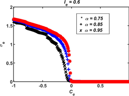
The standard deviation results of electrically coupled two conformable FHN neuron models for (α = 0.75, 0.85 and 0.95; I_e = 0.6)

Synchronization control of electrically coupled conformable FitzHugh-Nagumo neuron models

In the previous section, the electrical coupling of the conformable fractional FHN neuronal models has been discussed. And finally, it is shown that the coupling strength parameter C_e determines the synchronization status between neurons. However, in this case, interneuron synchronization may be disrupted as a result of an undesirable change in C_e. To eliminate this deficiency, a control is needed in which the synchronization of neurons can be determined independently of the parameter C_e. In this context, synchronization control methods have emerged. One of the most common and frequently used of these is the Lyapunov control method (Çimen et al. 2020). The controller applied in the Lyapunov control method does not cause any difference in the closed loop system, which is an important advantage, so that it can both provide information with synchronization error and ensure closed loop stability. On the other hand, the disadvantage of the Lyapunov control method is to choose the right Lyapunov function, because different function selections can lead to different effects (Kuang and Cong 2008; Nguyen and Hong 2011). Expressions of the electrically coupled conformable FHN neuron models with Lyapunov control method are given in (18).

$$\begin{array}{c}{T}_{t_0}^{\alpha }{y}_1=c\left(y_1-y_2+I_e-(y_1^3/3)\right)+C_e{\delta }_{12}{\gamma }_e(z_1,y_1)\\ T_{t_0}^{\alpha }{y}_2=(y_1-b{y}_2+a)/c\\ T_{t_0}^{\alpha }{z}_1=c\left(z_1-z_2+I_e-(z_1^3/3)\right)+C_e{\delta }_{21}{\gamma }_e(y_1,z_1)+K_C\\ T_{t_0}^{\alpha }{z}_2=(z_1-b{z}_2+a)/c\\ \end{array}$$ 18

where C_e is the coupling strength, (δ₁₂ = δ₂₁ = 1) are the coupling parameters and K_C is the controller. The electrical coupling functions γ_e(z₁, y₁) and γ_e(y₁, z₁) are z₁ − y₁ and y₁ − z₁, respectively. Here, the error variables e₁ and e₂ between the state variables of the two conformable FHN neurons are defined as follows.

$$\begin{array}{c}{e}_1=y_1-z_1\\ e_2=y_2-z_2\\ \end{array}$$ 19

If the conformable derivative operator is applied to both sides of (19), the equation set in (20) is obtained. If the expressions in (18) are substituted in (20), the differential equation set in (21) is derived.

$$\begin{array}{c}{T}_{t_0}^{\alpha }{e}_1=T_{t_0}^{\alpha }{y}_1-T_{t_0}^{\alpha }{z}_1\\ T_{t_0}^{\alpha }{e}_2=T_{t_0}^{\alpha }{y}_2-T_{t_0}^{\alpha }{z}_2\\ \end{array}$$ 20

$$\begin{array}{c}{T}_{t_0}^{\alpha }{e}_1=c\left(e_1-e_2-(y_1^3-z_1^3)/3\right)-2C_e{e}_1-K_C\\ T_{t_0}^{\alpha }{e}_2=(e_1-b{e}_2)/c\\ \end{array}$$ 21

At this point, let the positive Lyapunov function is defined as V_L = (e₁² + e₂²)/2. In this case, the conformable derivative of V_L is obtained by employing the properties given in Sect. "Mathematical definitions" as follows.

$$\begin{array}{c}{T}^{\alpha }{V}_L=\frac{1}{2}{T}^{\alpha }(e_1^2)+\frac{1}{2}{T}^{\alpha }(e_2^2)\\ =e_1{T}^{\alpha }{e}_1+e_2{T}^{\alpha }{e}_2\\ =e_1\left(c{e}_1-c{e}_2-c(y_1^3-z_1^3)/3-2C_e{e}_1-K_C\right)+e_2(e_1-b{e}_2)/c\\ \end{array}$$ 22

The controller expression K_C is obtained from (22) as follows.

$$K_C=c\left(e_1-e_2-(y_1^3-z_1^3)/3\right)-2C_e{e}_1+e_2/c$$ 23

The simulation results of the synchronization control of two electrically coupled conformable FHN neuron models by using the Lyapunov control method are presented in Fig. 6. It is clear from time responses and phase portraits that synchronous behavior is preserved with the Lyapunov control method regardless of the coupling strength parameter C_e. Moreover, it can be deduced from Fig. 6e that the standard deviation results close to zero and therefore the Lyapunov control method is effective. Thus, the Lyapunov control method applied to coupled integer order neuron models can also be successfully applied to coupled conformable neuron models. Another case is the impact of changing the fractional order α on synchronization of neurons under the same parameter conditions. The numerical simulation results obtained for different fractional orders (α = 0.95, 0.85 and 0.75) are shown in Fig. 7. It can be said from the related figure that as the fractional order α decreases, the standard deviation results decrease, so coupled conformable FHN neuron models with smaller fractional orders can exhibit more synchronous behavior. This is another difference between classical and conformable neuron models. In conformable neuron models, synchronization error in terms of the standard deviation results can be controlled with the fractional order.

Fig. 6.

a, c the time responses, b, d phase portraits and e standard deviation results of electrically coupled two conformable FHN neuron models with Lyapunov control method for (α = 0.95, I_e = 0.6)

Fig. 7.

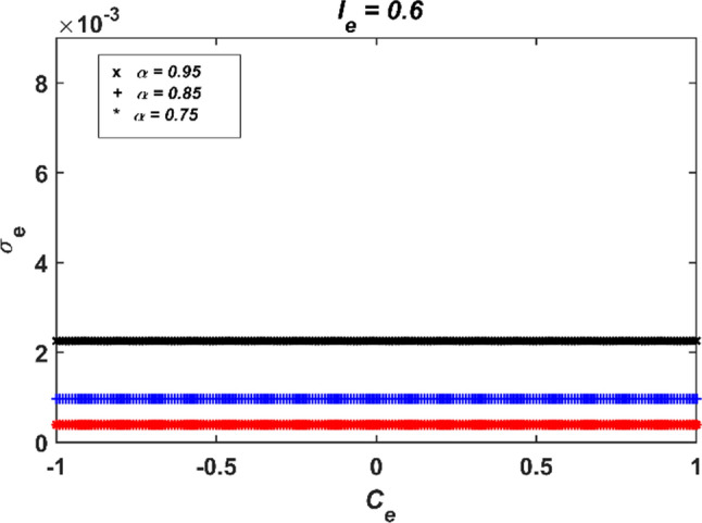
The standard deviation results of electrically coupled two conformable FHN neuron models with Lyapunov control method for (α = 0.95, 0.85 and 0.75; I_e = 0.6)

Texas Instrument F28335 Delfino digital signal processing (DSP) board has been used to experimentally verify the numerical simulation results attained in the previous sections. In order to make calculations on the DSP card and observe the state variables on the oscilloscope screen at the output, the amplitude levels of the relevant state variables (y₁, y₂, z₁ and z₂) have been shifted and scaled. At the same time, the conversion from digital to analog is provided with a digital to analog converter (DAC) group. The processing steps in detailed form for DSP implementation are presented in Table 1 algorithmically. The experimental hardware setup is depicted in Fig. 8.

Fig. 8.

The experimental setup for the verification of the obtained numerical simulation results

The measurement results of the conformable FHN neuronal model dynamics for the fractional order α = 0.95 and external stimulation I_e = 0.6 are presented in Fig. 9a. On the other hand, the measurement results obtained when the same I_e value and α = 0.85 are indicated in Fig. 9b. It can be apparently observed that the simulation results presented in Fig. 2 and the measurement results in Fig. 9 are in agreement with each other. Thus, it has been experimentally monitored that the frequency of the response of the FHN neuronal model increases with the decrease of the fractional order α.

Fig. 9.

The measurement results of the conformable FHN neuronal model dynamics for cases a α = 0.95, I_e = 0.6 and b α = 0.85, I_e = 0.6

On the other hand, the measurement results obtained for different C_e values of electrically coupled conformable FHN neuron models without synchronization control have been displayed in Fig. 10. It can be seen from the related figure that synchronous behavior has been monitored for C_e = 0.4 and asynchronous behavior has been observed for C_e =  − 0.4. Thus, it has also been experimentally observed that the synchronous behavior of two coupled neurons can be controlled depending on the value of the C_e parameter. Furthermore, the numerical simulation results shown in Fig. 4 have been also confirmed.

Fig. 10.

The measurement results of the electrically coupled conformable FHN neuron models without synchronization control for cases a α = 0.95, I_e = 0.6, C_e = 0.4 and b α = 0.95, I_e = 0.6, C_e =  − 0.4

Finally, the measurement results of electrically coupled conformable FHN neuron models with Lyapunov control method have been demonstrated in Fig. 11. It is clearly observed from the related figure that the neuron models exhibit synchronous behavior for both C_e =  − 0.4 and C_e = 0.4 values. Thus, the efficiency of the Lyapunov control method has been observed by performing the experimental verification of Fig. 6.

Fig. 11.

The measurement results of the electrically coupled conformable FHN neuron models with synchronization control for cases a α = 0.95, I_e = 0.6, C_e =  − 0.4 and b α = 0.95, I_e = 0.6, C_e = 0.4

To summarize the study in outline,

• (i)If the value of the parameter I_e is below a certain threshold value, the conformable FHN neuron model is at its resting state as in the classical integer-order neuron models.
• (ii)For the constant values of a, b, c and the stimulus I_e, the frequency of the dynamic response of the conformable FHN neuronal model increases as the fractional order α decreases. However, this inference is not possible in classical constant-order integer neuron models.
• (iii)For the constant values of a, b, c and the fractional order α, the frequency of the dynamic response of the conformable FHN neuronal model relatively increases as the external stimulus I_e increases. This observation is true for both classical and conformable neuron models.
• (iv)The coupling strength parameter C_e determines the synchronization state in electrically coupled conformable FHN neuron models. At positive values of C_e, responses of neurons approach synchronous behavior, while dynamics of neurons approach to asynchronous behavior at negative values of C_e. A similar situation is valid in classical integer-order neuron models.
• (v)By means of Lyapunov control method, electrically coupled conformable FHN neuron models exhibit synchronous behavior independent of the coupling strength parameter C_e. Thus, the Lyapunov control method used for the coupled integer order neuron models can also be successfully applied to coupled conformable neuron models.

Conclusions

In this work, a fractional conformable derivative based biological neuron model has been discussed. The ADM method has been used for numerical simulation studies. In numerical simulations, FHN neuron behavior has been examined in detail for different situations by changing the fractional order and external excitation current. In addition, electrical coupling of two FHN neurons has been performed and the effect of coupling strength parameter on coupling status has been evaluated. Moreover, the effectiveness of the Lyapunov control method has been investigated for the synchronous behavior of two neurons independent of the coupling strength parameter. Finally, the numerical simulation results have also been experimentally verified on the Texas Instrument DSP board. All these results reveal that the fractional order α can be considered as a separate bifurcation parameter and especially it affects the frequency of the response of the FHN neuron model. In this context, the effect of the definition of conformable derivative on the dynamics of different biological neuron models can also be discussed in future studies.

Data availability

Data sharing not applicable to this article as no datasets were generated or analyzed during the current study.

Declarations

Conflict of interest

The author declare that they have no conflict of interest.

References

- AbdelAty AM, Fouda ME, Eltawil AM (2022) On numerical approximations of fractional-order spiking neuron models. Commun Nonlinear Sci Numer Simul 105:106078. 10.1016/j.cnsns.2021.106078 10.1016/j.cnsns.2021.106078 [DOI] [Google Scholar]
- Abdeljawad T (2015) On conformable fractional calculus. J Comput Appl Math 279:57–66. 10.1016/j.cam.2014.10.016 10.1016/j.cam.2014.10.016 [DOI] [Google Scholar]
- Adomian G (1991) A review of the decomposition method and some recent results for nonlinear equations. Comput Math Appl 21(5):101–127. 10.1016/0898-1221(91)90220-X 10.1016/0898-1221(91)90220-X [DOI] [Google Scholar]
- Aqil M, Hong KS, Jeong MY (2012) Synchronization of coupled chaotic FitzHugh–Nagumo systems. Commun Nonlinear Sci Numer Simul 17(4):1615–1627. 10.1016/j.matcom.2011.10.005 10.1016/j.matcom.2011.10.005 [DOI] [Google Scholar]
- Avcı D, Eroglu BBI, Özdemir N (2017) Conformable fractional wave-like equation on a radial symmetric plate. In: Babiarz A, Czornik A, Klamka J, Niezabitowski M (eds) A Theory and Applications of Non-integer Order Systems. Springer, Cham, pp 137–146. 10.1007/978-3-319-45474-0_13 [Google Scholar]
- Baleanu D, Diethelm K, Scalas E, Trujillo JJ (2012) Fractional calculus: models and numerical methods. World Sci. 10.1142/8180 10.1142/8180 [DOI] [Google Scholar]
- Bao B, Hu A, Bao H, Xu Q, Chen M, Wu H (2018) Three-dimensional memristive Hindmarsh-Rose neuron model with hidden coexisting asymmetric behaviors. Complexity. 10.1155/2018/3872573 10.1155/2018/3872573 [DOI] [Google Scholar]
- Bao H, Hu A, Liu W, Bao B (2019) Hidden bursting firings and bifurcation mechanisms in memristive neuron model with threshold electromagnetic induction. IEEE Trans Neural Netw Lear Syst 31(2):502–511. 10.1109/TNNLS.2019.2905137 10.1109/TNNLS.2019.2905137 [DOI] [PubMed] [Google Scholar]
- Cafagna D, Grassi G (2008) Bifurcation and chaos in the fractional-order Chen system via a time-domain approach. Int J Bifurcat Chaos 18(07):1845–1863. 10.1142/S0218127408021415 10.1142/S0218127408021415 [DOI] [Google Scholar]
- Cafagna D, Grassi G (2009) Hyperchaos in the fractional-order Rössler system with lowest-order. Int J Bifurcat Chaos 19(01):339–347. 10.1142/S0218127409022890 10.1142/S0218127409022890 [DOI] [Google Scholar]
- Chow CC, Kopell N (2000) Dynamics of spiking neurons with electrical coupling. Neural Comput 12(7):1643–1678. 10.1162/089976600300015295 10.1162/089976600300015295 [DOI] [PubMed] [Google Scholar]
- Chung WS (2015) Fractional Newton mechanics with conformable fractional derivative. J Comput Appl Math 290:150–158. 10.1016/j.cam.2015.04.049 10.1016/j.cam.2015.04.049 [DOI] [Google Scholar]
- Çimen Z, Korkmaz N, Altuncu Y, Kılıç R (2020) Evaluating the effectiveness of several synchronization control methods applying to the electrically and the chemically coupled hindmarsh-rose neurons. Biosystems 198:104284. 10.1016/j.biosystems.2020.104284 10.1016/j.biosystems.2020.104284 [DOI] [PubMed] [Google Scholar]
- Daftardar-Gejji V, Bhalekar S (2008) Solving multi-term linear and non-linear diffusion–wave equations of fractional order by Adomian decomposition method. Appl Math Comput 202(1):113–120. 10.1016/j.amc.2008.01.027 10.1016/j.amc.2008.01.027 [DOI] [Google Scholar]
- Dalir M, Bashour M (2010) Applications of fractional calculus. Appl Math Sci 4(21):1021–1032 [Google Scholar]
- Dayan P, Abbott LF (2005) Theoretical neuroscience: computational and mathematical modeling of neural systems. MIT press [Google Scholar]
- Drapaca C (2016) Fractional calculus in neuronal electromechanics. J Mech Mater Struct 12(1):35–55. 10.2140/jomms.2017.12.35 10.2140/jomms.2017.12.35 [DOI] [Google Scholar]
- Duan JS, Rach R, Baleanu D, Wazwaz AM (2012) A review of the Adomian decomposition method and its applications to fractional differential equations. Commun Fract Calc 3(2):73–99 [Google Scholar]
- FitzHugh R (1969) Mathematical models for excitation and propagation in nerve. In: Schawn HP (ed) Biol Eng. McGraw-Hill, New York, pp 1–85 [Google Scholar]
- He S, Sun K, Mei X, Yan B, Xu S (2017) Numerical analysis of a fractional-order chaotic system based on conformable fractional-order derivative. Eur Phys J plus 132(36):1–11. 10.1140/epjp/i2017-11306-3 10.1140/epjp/i2017-11306-3 [DOI] [Google Scholar]
- He S, Banerjee S, Yan B (2018) Chaos and symbol complexity in a conformable fractional-order memcapacitor system. Complexity 2018:4140762. 10.1155/2018/4140762 10.1155/2018/4140762 [DOI] [Google Scholar]
- He S, Sun K, Wang H (2019) Dynamics and synchronization of conformable fractional-order hyperchaotic systems using the Homotopy analysis method. Commun Nonlinear Sci Numer Simul 73:146–164. 10.1016/j.cnsns.2019.02.007 10.1016/j.cnsns.2019.02.007 [DOI] [Google Scholar]
- Hindmarsh JL, Rose RM (1984) A model of neural bursting using three couple first order differential equations. Proc R Soc Lond Biol Sci 221(1222):87–102. 10.1098/rspb.1984.0024 10.1098/rspb.1984.0024 [DOI] [PubMed] [Google Scholar]
- Hodgkin A, Huxley A (1952) A quantitative description of membrane current and its application to conduction and excitation in nerve. J Physiol 117:500–544. 10.1113/jphysiol.1952.sp004764 10.1113/jphysiol.1952.sp004764 [DOI] [PMC free article] [PubMed] [Google Scholar]
- Ionescu C, Lopes A, Copot D, Machado JT, Bates JH (2017) The role of fractional calculus in modeling biological phenomena: a review. Commun Nonlinear Sci Numer Simul 51:141–159. 10.1016/j.cnsns.2017.04.001 10.1016/j.cnsns.2017.04.001 [DOI] [Google Scholar]
- İskender Eroğlu BB, Avci D, Özdemir N (2017) Optimal control problem for a conformable fractional heat conduction equation. Acta Phys Polonica A 132:658–662. 10.12693/APhysPolA.132.658 10.12693/APhysPolA.132.658 [DOI] [Google Scholar]
- Izhikevich EM (2003) Simple model of spiking neurons. IEEE Trans Neural Netw 14(6):1569–1572. 10.1109/tnn.2003.820440 10.1109/tnn.2003.820440 [DOI] [PubMed] [Google Scholar]
- Jun D, Guang-Jun Z, Yong X, Hong Y, Jue W (2014) Dynamic behavior analysis of fractional-order Hindmarsh-Rose neuronal model. Cogn Neurodyn 8(2):167–175. 10.1007/s11571-013-9273-x 10.1007/s11571-013-9273-x [DOI] [PMC free article] [PubMed] [Google Scholar]
- Kandel ER, Schwartz JH, Jessell TM (2000) Principles of neural science. McGraw-Hill, New York [Google Scholar]
- Kaslik E, Sivasundaram S (2012) Nonlinear dynamics and chaos in fractional-order neural networks. Neural Netw 32:245–256. 10.1016/j.neunet.2012.02.030 10.1016/j.neunet.2012.02.030 [DOI] [PubMed] [Google Scholar]
- Khalil R, Al Horani M, Yousef A, Sababheh M (2014) A new definition of fractional derivative. J Comput Appl Math 264:65–70. 10.1016/j.cam.2014.01.002 10.1016/j.cam.2014.01.002 [DOI] [Google Scholar]
- Korkmaz N, Öztürk İ, Kilic R (2016) Multiple perspectives on the hardware implementations of biological neuron models and programmable design aspects. Turk J Electr Eng Comput Sci 24(3):1729–1746. 10.3906/elk-1309-5 10.3906/elk-1309-5 [DOI] [Google Scholar]
- Korkmaz N, Saçu İE (2022) An alternative perspective on determining the optimum fractional orders of the synaptic coupling functions for the simultaneous neural patterns. Nonlinear Dyn 110:3791–3806. 10.1007/s11071-022-07782-z 10.1007/s11071-022-07782-z [DOI] [Google Scholar]
- Kuang S, Cong S (2008) Lyapunov control methods of closed quantum systems. Automatica 44(1):98–108. 10.1016/j.automatica.2007.05.013 10.1016/j.automatica.2007.05.013 [DOI] [Google Scholar]
- Li JS, Dasanayake I, Ruths J (2013) Control and synchronization of neuron ensembles. IEEE Trans Autom Control 58(8):1919–1930. 10.1109/TAC.2013.2250112 10.1109/TAC.2013.2250112 [DOI] [Google Scholar]
- Lu Q, Gu H, Yang Z, Shi X, Duan L, Zheng Y (2008) Dynamics of firing patterns, synchronization and resonances in neuronal electrical activities: experiments and analysis. Acta Mech Sin 24(6):593–628. 10.1007/s10409-008-0204-8 10.1007/s10409-008-0204-8 [DOI] [Google Scholar]
- Lundstrom BN, Higgs MH, Spain WJ, Fairhall AL (2008) Fractional differentiation by neocortical pyramidal neurons. Nat Neurosci 11:1335–1342. 10.1038/nn.2212 10.1038/nn.2212 [DOI] [PMC free article] [PubMed] [Google Scholar]
- Machado JT, Kiryakova V, Mainardi F (2011) Recent history of fractional calculus. Commun Nonlinear Sci Numer Simul 16(3):1140–1153. 10.1016/j.cnsns.2010.05.027 10.1016/j.cnsns.2010.05.027 [DOI] [Google Scholar]
- Malik SA, Mir AH (2020) FPGA realization of fractional order neuron. Appl Math Model 81:372–385. 10.1016/j.apm.2019.12.008 10.1016/j.apm.2019.12.008 [DOI] [Google Scholar]
- McCulloch WS, Pits WH (1943) A logical calculus of ideas immanent innervous activity. Bull Math Biophys 5:115–133. 10.1007/BF02478259 10.1007/BF02478259 [DOI] [Google Scholar]
- Mondal A, Sharma SK, Upadhyay RK, Mondal A (2019) Firing activities of a fractional-order FitzHugh-Rinzel bursting neuron model and its coupled dynamics. Sci Rep 9(1):1–11. 10.1038/s41598-019-52061-4 10.1038/s41598-019-52061-4 [DOI] [PMC free article] [PubMed] [Google Scholar]
- Morris C, Lecar H (1981) Voltage oscillations in the barnacle giant muscle fiber. Biophys J 35:193–213. 10.1016/S0006-3495(81)84782-0 10.1016/S0006-3495(81)84782-0 [DOI] [PMC free article] [PubMed] [Google Scholar]
- Nguyen LH, Hong KS (2011) Synchronization of coupled chaotic FitzHugh–Nagumo neurons via Lyapunov functions. Math Comput Simul 82(4):590–603. 10.1016/j.matcom.2011.10.005 10.1016/j.matcom.2011.10.005 [DOI] [Google Scholar]
- Pérez JES, Gómez-Aguilar JF, Baleanu D, Tchier F (2018) Chaotic attractors with fractional conformable derivatives in the Liouville-Caputo sense and its dynamical behaviors. Entropy 20:384. 10.3390/e20050384 10.3390/e20050384 [DOI] [PMC free article] [PubMed] [Google Scholar]
- Podlubny I (1998) Fractional differential equations: an introduction to fractional derivatives, fractional differential equations, to methods of their solution and some of their applications. Elsevier [Google Scholar]
- Purves D, Augustine GJ, Fitzpatrick D, Hall WC, Lamantia AS, Mcnamara JO, Williams SM (2004) Neuroscience, 3rd edn. Sinauer Associates Inc, USA [Google Scholar]
- Ray SS (2009) Analytical solution for the space fractional diffusion equation by two-step Adomian decomposition method. Commun Nonlinear Sci Numer Simul 14(4):1295–1306. 10.1016/j.cnsns.2008.01.010 10.1016/j.cnsns.2008.01.010 [DOI] [Google Scholar]
- Ruan J, Sun K, Mou J, He S, Zhang L (2018) Fractional-order simplest memristor-based chaotic circuit with new derivative. Eur Phys J plus 133(3):1–12. 10.1140/epjp/i2018-11828-0 10.1140/epjp/i2018-11828-0 [DOI] [Google Scholar]
- Shi M, Wang Z (2014) Abundant bursting patterns of a fractional-order Morris-Lecar neuron model. Commun Nonlinear Sci Numer Simul 19(6):1956–1969. 10.1016/j.cnsns.2013.10.032 10.1016/j.cnsns.2013.10.032 [DOI] [Google Scholar]
- Song L, Wang W (2013) A new improved Adomian decomposition method and its application to fractional differential equations. Appl Math Model 37(3):1590–1598. 10.1016/j.apm.2012.03.016 10.1016/j.apm.2012.03.016 [DOI] [Google Scholar]
- Soudry D, Meir R (2012) Conductance-based neuron models and the slow dynamics of excitability. Front Comput Neurosci 6:4. 10.3389/fncom.2012.00004 10.3389/fncom.2012.00004 [DOI] [PMC free article] [PubMed] [Google Scholar]
- Storace M, Linaro D, de Lange E (2008) The Hindmarsh-Rose neuron model: bifurcation analysis and piecewise-linear approximations. Chaos Interdiscip J Nonlinear Sci 18(3):033128. 10.1063/1.2975967 10.1063/1.2975967 [DOI] [PubMed] [Google Scholar]
- Teka W, Marinov TM, Santamaria F (2014) Neuronal spike timing adaptation described with a fractional leaky integrate-and-fire model. PLoS Comput Biol 10(3):e1003526 10.1371/journal.pcbi.1003526 [DOI] [PMC free article] [PubMed] [Google Scholar]
- Teka WW, Upadhyay RK, Mondal A (2017) Fractional-order leaky integrate-and-fire model with long-term memory and power-law dynamics. Neural Netw 93:110–125. 10.1016/j.neunet.2017.05.007 10.1016/j.neunet.2017.05.007 [DOI] [PubMed] [Google Scholar]
- Teka WW, Upadhyay RK, Mondal A (2018) Spiking and bursting patterns of fractional-order Izhikevich model. Commun Nonlinear Sci Numer Simul 56:161–176. 10.1016/j.cnsns.2017.07.026 10.1016/j.cnsns.2017.07.026 [DOI] [Google Scholar]
- Tolba MF, Elsafty AH, Armanyos M, Said LA, Madian AH, Radwan AG (2019) Synchronization and FPGA realization of fractional-order Izhikevich neuron model. Microelectron J 89:56–69. 10.1016/j.mejo.2019.05.003 10.1016/j.mejo.2019.05.003 [DOI] [Google Scholar]
- Usha K, Subha PA (2019) Collective dynamics and energy aspects of star-coupled Hindmarsh-Rose neuron model with electrical, chemical and field couplings. Nonlinear Dyn 96(3):2115–2124. 10.1007/s11071-019-04909-7 10.1007/s11071-019-04909-7 [DOI] [Google Scholar]
- Valenti D, Augello G, Spagnolo B (2008) Dynamics of a FitzHugh-Nagumo system subjected to autocorrelated noise. Eur Phys J B 65(3):443–451. 10.1140/epjb/e2008-00315-6 10.1140/epjb/e2008-00315-6 [DOI] [Google Scholar]
- Wazwaz AM (2000) A new algorithm for calculating Adomian polynomials for nonlinear operators. Appl Math Comput 111(1):33–51. 10.1016/S0096-3003(99)00063-6 10.1016/S0096-3003(99)00063-6 [DOI] [Google Scholar]
- Wilson HR, Cowan JD (1972) Excitatory and inhibitory interactions in localized populations of model neurons. Biophys J 12(1):1–24. 10.1016/S0006-3495(72)86068-5 10.1016/S0006-3495(72)86068-5 [DOI] [PMC free article] [PubMed] [Google Scholar]
- Xia S, Qi-Shao L (2005) Firing patterns and complete synchronization of coupled Hindmarsh-Rose neurons. Chin Phys 14(1):77. 10.1088/1009-1963/14/1/016 10.1088/1009-1963/14/1/016 [DOI] [Google Scholar]
- Zhang JQ, Huang SF, Pang ST, Wang MS, Gao S (2015) Synchronization in the uncoupled neuron system. Chin Phys Lett 32(12):9–13. 10.1088/0256-307x/32/12/120502 10.1088/0256-307x/32/12/120502 [DOI] [Google Scholar]
Associated Data
This section collects any data citations, data availability statements, or supplementary materials included in this article.
Data Availability Statement