Sidelobes and sideband minimization in time-modulated array antenna based on chaotic exchange nonlinear dandelion optimization algorithm

Abstract

Time-modulated array antenna (TMAA) is a new type of array antenna based on time modulation technology. By introducing "time" as the fourth dimensional design freedom into the design of conventional array antennas in three-dimensional space, the array antenna has time modulation characteristics, which better controls the radiation characteristics of the array antenna and achieves the best far-field radiation pattern synthesis. This paper designs a Time-modulated linear array (TMLA) with low sidelobe level (SLL) and low sideband level (SBL) based on the chaotic exchange nonlinear dandelion optimization (CENDO) algorithm. Three optimization methods are studied: firstly, determining the optimal on-time (τ_nn) for each array element; The second is to determine the optimal on-time (τ_nn) and optimal uniform array element spacing (d) for each array element; The third is to determine the optimal opening time (t_on), closing time (t_off), and optimal uniform array element spacing (d) for each array element. To achieve simultaneous reduction of sidelobe level and suppression of harmonic interference. The same array model contains different harmonic frequency radiation. In this article, we only considered two harmonic frequencies, namely the first sideband frequency and the second sideband frequency. Because the harmonic of other sideband frequencies has a very small impact on the radiation of the fundamental wave, it can be ignored. To demonstrate the stronger ability of the CENDO algorithm in optimizing Time-modulated array antennas, and in line with the principle of fairness and impartiality, this paper also simulates different Time-modulated array models and compares the results of the CENDO algorithm with other published literature. It is concluded that this study shows lower SLL and lower SBL in different models. This provides a more scientific and accurate explanation of the superiority of the CENDO algorithm compared to other algorithms in the field of antenna optimization in electromagnetics. At the same time, this also provides great research value and fundamental support for designing high-performance Time-modulated array antennas in subsequent engineering applications.

Introduction

An antenna is a transformer used to propagate electromagnetic waves. According to the IEEE standard definition, antennas are described as means of "transmitting or receiving radio waves"¹. Fields such as radio communication, broadcasting, television, radar, navigation, electronic countermeasures, remote sensing and radio astronomy all rely on antennas for their operations. In the new era, due to the expanding business volume in the electromagnetic environment, a single antenna is no longer able to meet the required directional gain. To enhance the radiation pattern of the antenna², a lot of research has been conducted on the design and synthesis of array antennas, to design array antennas with lower sidelobe level (SLL) and narrower half-power beamwidth (HPBW)³. In the early stages of research, people only used traditional analysis methods to model the excitation, such as using Taylor polynomials and Chebyshev polynomials to allocate the excitation amplitude^4,5, and using the conical amplitude distribution of attenuators to determine the excitation amplitude. These methods are often cumbersome and inefficient, and any small design defects may lead to extremely poor results⁶. Therefore, with the deepening of research, more and more swarm intelligence optimization algorithms are being used in the field of designing array antennas, and compared to traditional analysis methods, these evolutionary algorithms can achieve better antenna radiation characteristics. For example, genetic algorithm (GA)³, differential evolution (DE) algorithm^2,6,7, particle swarm optimization (PSO) algorithm^8,9, comprehensive learning particle swarm optimization (CLPSO) algorithm¹⁰, chaotic particle swarm optimization (CPSO) algorithm ¹¹, cat swarm optimization (CSO) algorithm¹², harmony search (HS)¹³, taboo search (TS)¹⁴, cuckoo optimization algorithm (COA)¹⁵ are widely used to design linear array antenna (LAA), using spider monkey optimization (SMO) algorithm¹⁶, the firefly algorithm (FFA)¹⁷, enhanced firefly algorithm (EFA)¹⁸, flower pollination algorithm (FPA)¹⁹, invasive weed optimization (IWO) algorithm²⁰, and grey wolf optimization (GWO) algorithm^21,22 for linear array antenna (LAA) design and radiation pattern synthesis. However, using these methods to design LAA still has some drawbacks, such as unstable excitation current weights and large dynamic range ratio. It is also difficult to simultaneously reduce SLL and improve directionality, so it is not easy to synthesize the optimal radiation pattern, as the decrease in SLL results in a decrease in directionality, which conflicts with each other. In addition, to achieve beam control in linear array antennas, phased arrays, which are limited to specialist military systems, necessitate the use of costly digital phase shifters to optimize the phase of the array elements. In order to overcome these limitations and drawbacks, Time-modulated array antennas have emerged, and their advantages over traditional array antennas have attracted extensive research from antenna designers in recent years.

TMAA is a new type of array antenna using time modulation technology, which introduces the fourth dimension—time in the design of array antenna. It not only reduces system costs and errors but also has greater flexibility, and the SLL is greatly reduced, better controlling the radiation characteristics of the array antenna. Time-modulated array antennas use high-precision control to periodically turn on and off the radio frequency (RF) switches, which is part of the feeding network that connects the adder to the output of the array components. This allows the antenna to achieve array weighting. By using uniform or non-uniform excitation to achieve adjustable switch configurations, extremely low or ultra-low SLL with improved radiation characteristics can be obtained^23,24. In addition, time modulation will continue to be applied in fields such as tracking radar systems²⁵, path finding²⁶, arrival direction evaluation²⁷, and automatic beam steering^28,29. Figure 1 shows the general structure of a Time-modulated array antenna. If all element switches are closed, the array behaves as a traditional linear array³⁰. On the contrary, it is a Time-modulated array. However, there is a common problem with Time-modulated array antennas, which is that they generate harmonics or sidebands in multiples of the switching frequency^31–33. And these unexpected harmonics will waste energy and cause interference to the fundamental wave and even other parts of the radio spectrum. Therefore, we need to determine the appropriate time series by appropriately opening and closing each array element to suppress harmonic waste and interference and improve the performance of the array. More specifically, various evolutionary algorithms are used to optimize time, such as genetic algorithm (GA)³⁰, particle swarm optimization (PSO) algorithm³⁴, and differential evolution (DE) algorithm³⁵, to determine the optimal time series and obtain the synthesis of patterns with low SLL and low SBL. This paper will use the CENDO algorithm to design and optimize the TMLA problem.

Figure 1.

General structure diagram of Time-modulated array.

The process of the CENDO algorithm is detailed in Section "The CENDO algorithm" of this paper. In Section "The theory and design equations of TMLA", the basic structure and theoretical knowledge of TMLA are introduced. Then, in Section "Results and discussions", three distinct optimization schemes are utilized to design the directional pattern synthesis of a Time-modulated array using the CENDO algorithm, and the results are compared with the design results of other algorithms to verify the effectiveness of the CENDO algorithm in TMLA synthesis. Finally, the summary of the paper is provided in Section "Summary".

The CENDO algorithm

The CENDO algorithm is an improved swarm intelligence optimization algorithm based on the dandelion optimization (DO) algorithm³⁶, inspired by the growth and reproduction process of dandelions. The CENDO algorithm has made three improvements on the basis of the DO algorithm: firstly, in the initialization stage, a logistic-tent chaotic mapping is introduced to generate the initial population, making the population distribution more uniform; The second is the iterative exchange in the rising stage to prevent falling into local optima; The third is to introduce nonlinear factors during the landing stage, being able to find the optimal solution more accurately enhances the optimization ability.

In the CENDO algorithm, the position of dandelion represents a possible solution to the optimization problem, and the growth and reproduction process of dandelion is divided into three stages: ascending, descending, and landing. Each stage requires an iteration of dandelion position updates, and finally finds the most suitable position for dandelion growth and reproduction, which is the optimal solution in the optimization problem. This section mainly introduces the process and specific expressions of the CENDO algorithm. The flowchart of the CENDO algorithm is shown in Fig. 2.

Figure 2.

The flowchart of CENDO algorithm.

Chaos initialization–logistic-tent mapping

Logistic mapping is a unimodal mapping that is a pseudo random sequence with the advantages of randomness and the high sensitivity of initial values unique to chaos³⁷. The logistic mapping divides the mapping independent variable interval into reasonable segments, expands the chaotic control parameter area, expands the coverage range to the entire control parameter range, and makes the generated sequence distribution more uniform. The following is the mathematical expression for logistic mapping:

$$X_{\text{n}+1}=X_n\mu \left(1-X_n\right)$$ 1

where X_n represents the result of the iteration, and the range of X_n is (0, 1). μ is a branching parameter used to control the chaotic state of the logistic mapping, with a range of (0, 4).

Tent mapping is a segmented linear mapping that has a somewhat excellent autocorrelation, uniform probability distribution, and power spectral density³⁸. It produces a chaotic sequence with good distribution and randomness. The initial population distribution can be adjusted more uniform based on these features, which will help the algorithm find the global ideal value. The mathematical expression for tent mapping is as follows:

$${\text{x}}_{\text{n}+1}=\left\{\begin{array}{c}c{x}_n/2,x_n<\frac{1}{2}\\ c\left(1-x_n\right)/2,x_n\ge \frac{1}{2}\\ \end{array}\right)$$ 2

where x_n refers to the variable of the problem, c is a chaotic parameter. When x_n belongs to [0, 1] and c belongs to^2,4, the system is in a chaotic state.

Tent mapping and logistic mapping are mutually topological conjugate maps. In order to combine the advantages of the two, the algorithm used in this paper utilizes the logic tent combination mapping method³⁹, which combines the complex chaotic dynamics characteristics of high zero sensitivity and randomness of logistic mapping with the stronger autocorrelation, better distribution and randomness of tent mapping. In this way, during algorithm initialization, the population is more evenly distributed in the search space, which is beneficial for improving the optimization efficiency and solving accuracy of the algorithm. The mathematical expression for initialization is as follows:

$$X_{n+1}=\left\{\begin{array}{c}\left[\beta x_n\left(1-x_n\right)+\left(\left(4-\beta \right)/2\right)x_n\right]mod1,x_n<1/2\\ \left[\beta x_n\left(1-x_n\right)+\left(\left(4-\beta \right)\left(1-{\text{x}}_{\text{n}}\right)/2\right)\right]mod1,x_n\ge 1/2\\ \end{array}\right)$$ 3

where X_n+1 is system variable, β is control parameter with a range of [0, 2], and $x_{\text{n}}\in \left[0,1\right]$.

In the synthesis application of array antennas, the chaos initialization in the CENDO algorithm can generate many chaotic sequences with good randomness, providing a good research model for generating high-quality initial populations³⁹. As shown in Fig. 3, we can see that the initial solution is distributed as evenly as possible in the solution space.

Figure 3.

The population distribution diagram (left) and histogram (right) of the Logistic-tent chaotic mapping.

Dandelion ascent stage

During the rising stage of dandelion, it is influenced by factors such as wind speed, air humidity, and other variables, and is divided into two types: sunny and rainy days. The following describes the optimization iteration process and mathematical model of dandelion in these two situations.

Sunny weather condition

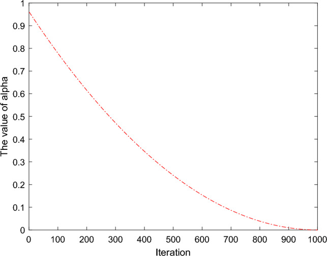
In sunny days, dandelions have a better chance of flying to further search areas for exploration, so it is required that the step parameter k of the iterative formula in this case be larger, so that more feasible solutions can be obtained within a larger search range, and the optimal solution can be found more accurately to avoid falling into local optima. The mathematical expression for the evolutionary iteration of dandelion in this case is as follows:

$$X_{\text{t}+1}=\text{k}\times X_{\text{t}}$$ 4

where k is used to adjust the search area of dandelion to obtain different search steps, which is determined by Eq. (5). Figure 4 shows the variation curve of k.

$$\begin{array}{c}\text{q}=\frac{1}{T^2-2T+1}{\text{t}}^2-\frac{2}{T^2-2T+1}\text{t}+1+\frac{1}{T^2-2T+1}\\ \text{k}=1-\text{rand}\left(\right)\times \text{q}\\ \end{array}$$ 5

where q is an adjustment factor determined by the current iteration number t and the maximum iteration number T, used to calculate k.

Figure 4.

The iterative curve graph of k.

Rainy weather condition

In rainy days, it is difficult for dandelions to fly further for breeding. They only need to be developed in small neighborhoods near them. In this case, the step parameter α value requiring an iterative formula is relatively small, to more accurately find the most suitable optimal solution within the nearby small neighborhood range. The mathematical expression for the evolutionary iteration of dandelion is as follows:

$$X_{\text{t}+1}=X_{\text{t}}+\alpha \times {\text{v}}_{\text{x}}\times {\text{v}}_{\text{y}}\times lnY\times \left(X_{\text{s}}-X_{\text{t}}\right)$$ 6

where α is an adaptive parameter used to modify the search step length, Fig. 5 shows the variation curve of α, its mathematical expression is as follows:

$$\alpha =\text{rand}\left(\right)\times \left(\frac{1}{T^2}{\text{t}}^2-\frac{2}{T}\text{t}+1\right)$$ 7

Figure 5.

The iterative curve graph of α.

In this case, dandelion propagates in a spiral pattern, where v_x and v_y are the two parts of the force generated by the formed vortex. The mathematical expression is as follows:

$$\begin{array}{c}\text{r}=\frac{1}{{\text{e}}^{\theta }}\\ {\text{v}}_{\text{x}}=\text{r}\times cos\theta \\ v_y=r\times sin\theta \\ \end{array}$$ 8

In Eq. (8), θ is a random number between [− π, π]. r represents the rising vortex distance.

where lnY denotes a lognormal distribution subject to $\mu$ = 0 and ${\sigma }^2$ = 1, and its mathematical formula is as follows:

$$lnY=\left\{\begin{array}{c}\frac{1}{\text{y}\sqrt{2\pi }}exp\left[-\frac{1}{2{\sigma }^2}{\left(ln\text{y}\right)}^2\right],y\ge 0\\ 0,y<0\\ \end{array}\right)$$ 9

In Eq. (9), y represents the standard normal distribution N (0, 1).

where X_s represents a position in the randomly selected search space during the iteration process, and Eq. (10) provides its mathematical expression.

$$X_{\text{s}}=\text{rand}\left(1,Dim\right)\times \left(UB-LB\right)+LB$$ 10

In Eq. (10), rand generates a random matrix with 1 row Dim (dimension of the problem) column between 0 and 1. LB and UB represent the lower and upper bounds of the problem. The mathematical expressions for LB and UB are as follows:

$$LB=\left[{\text{lb}}_1,...,l{b}_{D\text{im}}\right],UB=\left[{\text{ub}}_1,...,u{b}_{D\text{im}}\right]$$ 11

Dandelion descent stage

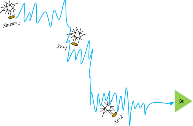
After the ascent stage is completed, the dandelion iteration enters the descent stage, during which the dandelion needs to use the average information of the ascent stage for iteration. The mathematical expression for this stage is as follows:

$$X_{\text{t}+1}=X_{\text{t}}-\alpha \times {\beta }_{\text{t}}\times \left(X_{\text{mean}\_t}-\alpha \times {\beta }_t\times X_t\right)$$ 12

where β_t is a random number from the standard normal distribution, representing Brownian motion⁴⁰, used to describe the trajectory of dandelions. Figure 6 depicts the trajectory of Brownian motion of dandelions. X_{mean_t} represents the average information of the rising stage, and its mathematical expression is as follows:

$$X_{\text{mean}\_t}=\frac{1}{N}\sum _{i=1}^N{X}_i$$ 13

Figure 6.

Iterative trajectory of dandelion in descent stage.

Dandelion landing stage

After the descent stage is completed, the dandelion begins to enter the landing stage. As the iteration progresses, the location information of dandelions is constantly updated. Due to the δ parameter continuing to increase, the search range in their neighborhood gradually narrows, which can effectively avoid crossing the optimal value and thus gradually approach the optimal position. Ultimately, the global optimal solution can be found. The mathematical expression of dandelion at this stage is as follows:

$$X_{\text{t}+1}=X_{\text{elite}}+\text{levy}\left(\lambda \right)\times \alpha \times \left(X_{\text{elite}}-X_{\text{t}}\times \delta \right)$$ 14

where X_elite represents the optimal position of dandelion in the current iteration. Levy ($\lambda$) represents the Levy flight function⁴¹, whose mathematical expression is given by Eq. (15). During this process, the Levy flight function allows dandelions to land in more distant places with a greater probability for neighborhood search, which helps the CENDO algorithm avoid local optima.

$$L\text{evy}\left(\lambda \right)=\text{s}\times \frac{\text{w}\times \sigma }{{\left|{\text{t}}_{\text{r}}\right|}^{\frac{1}{\beta }}}$$ 15

The parameters of the Levy flight function are set as follows, where the β value in the Eq. (15) is set to 1.5³⁶, s is set to 0.01³⁶, w and t_r are random values between [0, 1]³⁶. The Eq. (16) gives a mathematical expression of $\sigma$. This setting can enable the CENDO algorithm to quickly converge to the global optimal solution, achieving dynamic control and balance throughout the entire convergence process.

$$\sigma =\left(\frac{\mathrm{\Gamma }\left(1+\beta \right)\times sin\left(\frac{\pi \beta }{2}\right)}{\mathrm{\Gamma }\left(\frac{1+\beta }{2}\right)\times \beta \times 2^{\left(\frac{\beta -1}{2}\right)}}\right)$$ 16

In Eq. (14), δ parameter is a nonlinear growth factor added from [0, 2] to control the current position information of dandelion. Its mathematical expression is given by Eq. (17). Figure 7 describes the change curve of δ.

$$\delta =log\left(4\times \left(\frac{exp\left(2{\text{t}}^2/T^2\right)}{4}\right)\right)$$ 17

Figure 7.

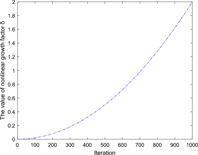
The iterative curve graph of δ.

Based on Fig. 7, we can see that its value shows a slow increasing trend. In the early stage of the iteration, the increase is slow, and its value is relatively small, so its neighborhood search range is relatively large and can search for the optimal value range faster; In the middle and later stages of the iteration, the increase is rapid, and its value is relatively large, so the search neighborhood is quickly reduced, which can more accurately find the optimal value. Therefore, this helps the CENDO algorithm find the best solution in a faster and more accurate way.

The theory and design equations of TMLA

This section describes the relevant theoretical knowledge of Time-modulated linear arrays (including symmetric and asymmetric Time-modulated arrays) and the corresponding mathematical model expressions under different time schemes. Figure 8 shows the model diagram of TMLA, which is connected to isotropic array elements using high-speed RF switches and placed along the x-axis.

Figure 8.

Model framework of standard N-element TMLA.

Symmetric time-modulation array

Figure 9 shows a typical structure of a linear array consisting of 2N isotropic sources arranged symmetrically and equidistant along the x-axis. The mathematical expression for the corresponding array factor of this traditional linear array antenna is as follows:

$$AF\left(\theta \right)=2\sum _{\text{n}=1}^N{I}_{\text{n}}{\text{e}}^{\text{j}\left(\text{nkd}cos\left(\theta \right)+{\phi }_{\text{n}}\right)}$$ 18

where I_n and φ_n represent the excitation amplitude and phase, respectively. k is the propagation constant (k = 2π/λ, with λ being the wavelength), θ represents the angle of the incident electromagnetic wave, d represents the distance between each array element, and N is the number of array elements.

Figure 9.

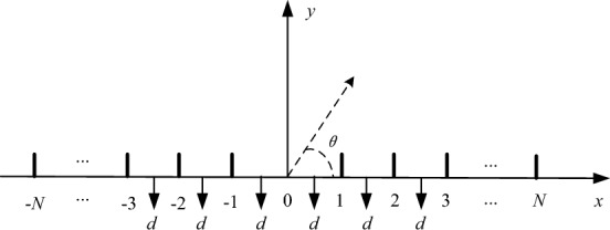
Model diagram of a linear array antenna.

If each array element is connected to a high-speed RF switch and these elements periodically change direction at a predetermined turn on-time, combined with the concept of time modulation, modify the expression of the array factor in Eq. (18) as follows⁴²:

$$AF\left(\theta ,t\right)={\text{e}}^{\text{j2}\pi {\text{f}}_0\text{t}}2\sum _{\text{n}=1}^N{I}_{\text{n}}{\text{U}}_{\text{n}}\left(\text{t}\right){\text{e}}^{\text{j}\left(\text{nkd}cos\left(\theta \right)+{\phi }_{\text{n}}\right)}$$ 19

In a Time-modulated array, each antenna is controlled by a switch, and the periodic switch on-time function U_n(t) is given by Eq. (20).

$$U_{\text{n}}\left(\text{t}\right)=\left\{\begin{array}{cc}1,\hfill & 0\le t\le {\tau }_n\\ 0,\hfill & \mathit{elsewhere}\end{array}\right)$$ 20

TMLA operates at the fundamental frequency of f₀, with a fundamental frequency period of T₀ (T₀ = 1/f₀). The time series function U_n(t) is periodic, and the modulation frequency f_p is much smaller than f₀ (i.e., f_p <  < f₀ and T_p >  > T₀, where T_p represents the modulation period). Now, instead of simultaneously exciting all elements, each element is "turned on" for a fixed duration of τ_m with a pulse repetition rate of f_p = 1/T_p; T_p is the pulse repetition period within the range of τ_m ≤ T_p > T₀, and the on-time of each antenna in TMLA is τ_n (0 ≤ τ_n ≤ T_p). Due to the periodicity of the function U_n(t), its periodic behavior can be expressed in the frequency domain as the following mathematical expression⁴².

$$U_{\text{n}}\left(t\right)=\sum _{m=-\infty }^{\infty }{b}_{\mathit{mn}}{e}^{j2\pi m{f}_{p}t}$$ 21

where, the mathematical expression for b_mn is as follows:

$${\text{b}}_{\text{mn}}=\frac{I_{\text{n}}{\tau }_{\text{n}}}{T_{\text{p}}}sin\text{c}\left(\pi {\text{mf}}_{\text{p}}{\tau }_{\text{n}}\right){\text{e}}^{-\text{j}\pi {\text{mf}}_{\text{p}}{\tau }_{\text{n}}}$$ 22

Equation (22) shows the complex excitation coefficient of the mth harmonic. Among them, m = 0 represents the fundamental wave, and the center frequency (f₀); m =  ± 1 represents the first harmonic, the first sideband frequency (f₀ + f_p); m =  ± 2 represents the second harmonic, the second sideband frequency (f₀ + 2f_p). And so on, m =  ± 3, …, ± ∞, represents higher-order harmonics.

By substituting Eqs. (21) and (22) into Eq. (19), the array factor of the Time-modulated array can be rewritten as Eq. (23).

$$AF\left(\theta ,t\right)=\sum _{\text{m}=-\infty }^{\infty }\sum _{\text{n}=1}^N{\text{2b}}_{\text{mn}}{\text{e}}^{\text{j2}\pi \left({\text{f}}_0+{\text{mf}}_{\text{p}}\right)\text{t}}{\text{e}}^{\text{j}\left(\text{nkd}cos\left(\theta \right)+{\phi }_{\text{n}}\right)}$$ 23

The expression of Eq. (23) includes mth harmonic frequency component (mf_p), which is the sum of infinite harmonic frequency modes. It is worth noting that the mathematical expression of the array factor for the m^th order sideband component can be written as follows⁴³:

$$A{F}_{\text{m}}\left(\theta ,t\right)={\text{e}}^{\text{j2}\pi \left({\text{f}}_0+{\text{mf}}_{\text{p}}\right)\text{t}}\sum _{\text{n}=1}^{N}2{\text{b}}_{\text{mn}}{\text{e}}^{\text{j}\left(\text{nkd}cos\left(\theta \right)+{\phi }_{\text{n}}\right)}$$ 24

From Eq. (24), we can also represent the array factor of the fundamental wave, the array factor of the first positive harmonic, and the array factor of the second positive harmonic, respectively. Their mathematical expression is as follows:

$$A{F}_0\left(\theta ,t\right)={\text{e}}^{\text{j2}\pi {\text{f}}_0\text{t}}\sum _{\text{n}=1}^{N}2\frac{I_{\text{n}}{\tau }_{\text{n}}}{T_{\text{p}}}{\text{e}}^{\text{j}\left(\text{nkd}cos\left(\theta \right)+{\phi }_{\text{n}}\right)}$$ 25

$$A{F}_1\left(\theta ,t\right)={\text{e}}^{\text{j2}\pi \left({\text{f}}_0+{\text{f}}_{\text{p}}\right)\text{t}}\sum _{\text{n}=1}^{N}2\frac{I_{\text{n}}{\tau }_{\text{n}}}{T_{\text{p}}}\text{sinc}\left(\pi {\text{f}}_{\text{p}}{\tau }_{\text{n}}\right){\text{e}}^{-\text{j}\pi {\text{f}}_{\text{p}}{\tau }_{\text{n}}}{\text{e}}^{\text{j}\left(\text{nkd}cos\left(\theta \right)+{\phi }_{\text{n}}\right)}$$ 26

$$A{F}_2\left(\theta ,t\right)={\text{e}}^{\text{j2}\pi \left({\text{f}}_0+2{\text{f}}_{\text{p}}\right)\text{t}}\sum _{\text{n}=1}^{N}2\frac{I_{\text{n}}{\tau }_{\text{n}}}{T_{\text{p}}}sin\text{c}\left(2\pi {\text{f}}_{\text{p}}{\tau }_{\text{n}}\right){\text{e}}^{-\text{j}2\pi {\text{f}}_{\text{p}}{\tau }_{\text{n}}}{\text{e}}^{\text{j}\left(\text{nkd}cos\left(\theta \right)+{\phi }_{\text{n}}\right)}$$ 27

Considering the uniform static excitation amplitude and phase, i.e. I_n = 1, φ_n = 0; The array factor expressions for fundamental wave, first harmonic, and second harmonic can be simplified as follows:

$$A{F}_0\left(\theta ,t\right)={\text{e}}^{\text{j2}\pi {\text{f}}_0\text{t}}\sum _{\text{n}=1}^{N}2\frac{{\tau }_{\text{n}}}{T_{\text{p}}}{\text{e}}^{\text{jnkd}cos\left(\theta \right)}$$ 28

$$A{F}_1\left(\theta ,t\right)={\text{e}}^{\text{j2}\pi \left({\text{f}}_0+{\text{f}}_{\text{p}}\right)\text{t}}\sum _{\text{n}=1}^{N}2\frac{{\tau }_{\text{n}}}{T_{\text{p}}}\text{sinc}\left(\pi {\text{f}}_{\text{p}}{\tau }_{\text{n}}\right){\text{e}}^{-\text{j}\pi {\text{f}}_{\text{p}}{\tau }_{\text{n}}}{\text{e}}^{\text{jnkd}cos\left(\theta \right)}$$ 29

$$A{F}_2\left(\theta ,t\right)={\text{e}}^{\text{j2}\pi \left({\text{f}}_0+2{\text{f}}_{\text{p}}\right)\text{t}}\sum _{\text{n}=1}^{N}2\frac{{\tau }_{\text{n}}}{T_{\text{p}}}sin\text{c}\left(2\pi {\text{f}}_{\text{p}}{\tau }_{\text{n}}\right){\text{e}}^{-\text{j}2\pi {\text{f}}_{\text{p}}{\tau }_{\text{n}}}{\text{e}}^{\text{jnkd}cos\left(\theta \right)}$$ 30

The above three expressions provide a method for calculating the array factor of a symmetric Time-modulation array at the fundamental frequency (f₀), the first harmonic frequency (f₀ ± f_p), and the second harmonic frequency (f₀ ± 2f_p), which can be used for synthesizing the desired radiation pattern.

Asymmetric time-modulation array

The theoretical knowledge of asymmetric Time-modulation arrays is basically the same as that of symmetric Time-modulation arrays, except that the array factor expressions of the fundamental wave and each harmonic are different. In an asymmetric Time-modulation array, the fundamental wave, as well as the array factors of the first and second positive harmonics, are expressed as follows:

$$A{F}_0\left(\theta ,t\right)={\text{e}}^{\text{j2}\pi {\text{f}}_0\text{t}}\sum _{\text{n}=1}^N\frac{{\tau }_{\text{n}}}{T_{\text{p}}}{\text{e}}^{\text{j}\left(\text{n}-1\right)\text{kd}cos\left(\theta \right)}$$ 31

$$A{F}_1\left(\theta ,t\right)={\text{e}}^{\text{j2}\pi \left({\text{f}}_0+{\text{f}}_{\text{p}}\right)\text{t}}\sum _{\text{n}=1}^N\frac{{\tau }_{\text{n}}}{T_{\text{p}}}\text{sinc}\left(\pi {\text{f}}_{\text{p}}{\tau }_{\text{n}}\right){\text{e}}^{-\text{j}\pi {\text{f}}_{\text{p}}{\tau }_{\text{n}}}{\text{e}}^{\text{j}\left(\text{n}-1\right)\text{kd}cos\left(\theta \right)}$$ 32

$$A{F}_2\left(\theta ,t\right)={\text{e}}^{\text{j2}\pi \left({\text{f}}_0+2{\text{f}}_{\text{p}}\right)\text{t}}\sum _{\text{n}=1}^N\frac{{\tau }_{\text{n}}}{T_{\text{p}}}sin\text{c}\left(2\pi {\text{f}}_{\text{p}}{\tau }_{\text{n}}\right){\text{e}}^{-\text{j}2\pi {\text{f}}_{\text{p}}{\tau }_{\text{n}}}{\text{e}}^{\text{j}\left(\text{n}-1\right)\text{kd}cos\left(\theta \right)}$$ 33

Similarly, Eqs. (31), (32), and (33) can be used to achieve pattern synthesis of asymmetric time modulated arrays.

Different time optimization schemes

In the optimization design of TMLA, we can optimize the on-time (τ_n), it is also possible to optimize both the opening time (t₁) and closing time (t₂) simultaneously. The array factor expressions for each harmonic under different time optimization strategies are different. Below, an asymmetric time modulation array will be used to explain the above two schemes separately.

Switch configuration 1

Each switch is simultaneously on at 0 times, with only on-time (τ_n). The definition of the time series function U_n(t) in this scheme can be used as shown in Fig. 10. The on-time of each array element within the modulation period (T_p) is τ_n. The mathematical expression for U_n(t) under this scheme is provided by Eq. (20).

Figure 10.

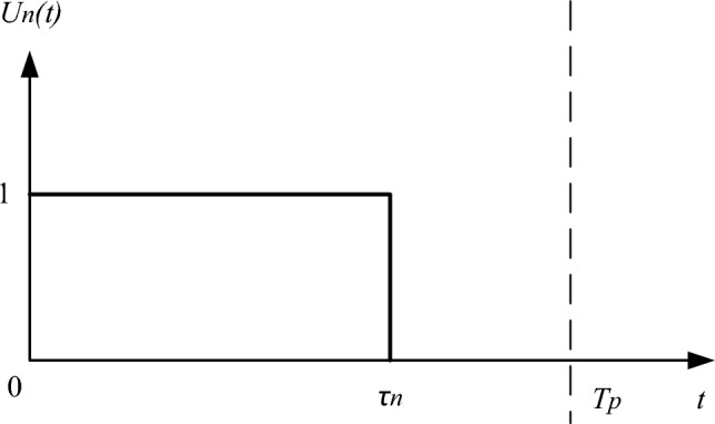
Time series diagram for switch configuration 1.

Similarly, we can also obtain the array factor expressions for the fundamental wave, first harmonic, and second harmonic in this case, which are given by Eqs. (31), (32), and (33), respectively.

In order to solve the comparability between data indicators and improve the optimization speed of the algorithm in subsequent simulations, we normalized the on-time (τ_n) of each array element. So, Eqs. (31), (32), and (33) are adjusted as follows:

$$A{F}_0\left(\theta ,t\right)={\text{e}}^{\text{j2}\pi {\text{f}}_0\text{t}}\sum _{\text{n}=1}^N{\tau }_{\text{nn}}{\text{e}}^{\text{j}\left(\text{n}-1\right)\text{kd}cos\left(\theta \right)}$$ 34

$$A{F}_1\left(\theta ,t\right)={\text{e}}^{\text{j2}\pi \left({\text{f}}_0+{\text{f}}_{\text{p}}\right)\text{t}}\sum _{\text{n}=1}^N{\tau }_{\text{nn}}\text{sinc}\left(\pi {\tau }_{\text{nn}}\right){\text{e}}^{-\text{j}\pi {\tau }_{\text{nn}}}{\text{e}}^{\text{j}\left(\text{n}-1\right)\text{kd}cos\left(\theta \right)}$$ 35

$$A{F}_2\left(\theta ,t\right)={\text{e}}^{\text{j2}\pi \left({\text{f}}_0+2{\text{f}}_{\text{p}}\right)\text{t}}\sum _{\text{n}=1}^N{\tau }_{\text{nn}}sin\text{c}\left(2\pi {\tau }_{\text{nn}}\right){\text{e}}^{-\text{j}2\pi {\tau }_{\text{nn}}}{\text{e}}^{\text{j}\left(\text{n}-1\right)\text{kd}cos\left(\theta \right)}$$ 36

where, τ_nn (τ_nn = τ_n/T_p) represents the normalized on-time. It is also one of the optimization variables in the experimental simulation part.

Switch configuration 2

Each switch is turned on and off at different times, with both opening time (t₁) and closing time (t₂). The definition of the time series function U_n(t) in this scheme is different, as shown in Fig. 11. The on-time of each array element within the modulation period (T_p) is still τ_n. The difference is that each switch is not uniformly turned on at the "0" times, requiring them to be turned on and off at different times to optimize the opening time (t₁) and closing time (t₂) of each array element. The mathematical expression for U_n(t) under this scheme is as follows:

$$U_{\text{n}}\left(\text{t}\right)=\left\{\begin{array}{c}1,0<t_1\le t\le t_2\le T_p\\ 0,elsewhere\\ \end{array}\right)$$ 37

Figure 11.

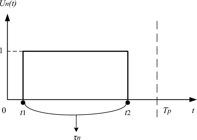
Time series diagram for switch configuration 2.

Based on the time series function under this scheme, we can derive that its Fourier excitation coefficient is adjusted from Eq. (22) to Eq. (38)⁴⁴. So, in this case, the array factors of the fundamental wave, first harmonic, and second harmonic also need to be changed accordingly, and their expressions are given by Eqs. (39), (40), and (41), respectively.

$${\text{b}}_{\text{mn}}=\frac{I_{\text{n}}\left({\text{t}}_2-t_1\right)}{T_{\text{p}}}sin\text{c}\left(\pi {\text{mf}}_{\text{p}}\left(t_2-t_1\right)\right){\text{e}}^{-\text{j}\pi {\text{mf}}_{\text{p}}\left(t_2+t_1\right)}$$ 38

$$A{F}_0\left(\theta ,t\right)={\text{e}}^{\text{j2}\pi {\text{f}}_0\text{t}}\sum _{\text{n}=1}^N\frac{\left({\text{t}}_2-{\text{t}}_1\right)}{T_{\text{p}}}{\text{e}}^{\text{j}\left(\text{n}-1\right)\text{kd}cos\left(\theta \right)}$$ 39

$$A{F}_1\left(\theta ,t\right)={\text{e}}^{\text{j2}\pi \left({\text{f}}_0+{\text{f}}_{\text{p}}\right)\text{t}}\sum _{\text{n}=1}^N\frac{\left({\text{t}}_2-{\text{t}}_1\right)}{T_{\text{p}}}\text{sinc}\left(\pi {\text{f}}_{\text{p}}\left({\text{t}}_2-{\text{t}}_1\right)\right){\text{e}}^{-\text{j}\pi {\text{f}}_{\text{p}}\left({\text{t}}_2+{\text{t}}_1\right)}{\text{e}}^{\text{j}\left(\text{n}-1\right)\text{kd}cos\left(\theta \right)}$$ 40

$$A{F}_2\left(\theta ,t\right)={\text{e}}^{\text{j2}\pi \left({\text{f}}_0+2{\text{f}}_{\text{p}}\right)\text{t}}\sum _{\text{n}=1}^N\frac{\left({\text{t}}_2-{\text{t}}_1\right)}{T_{\text{p}}}sin\text{c}\left(2\pi {\text{f}}_{\text{p}}\left({\text{t}}_2-{\text{t}}_1\right)\right){\text{e}}^{-\text{j}2\pi {\text{f}}_{\text{p}}\left({\text{t}}_2+{\text{t}}_1\right)}{\text{e}}^{\text{j}\left(\text{n}-1\right)\text{kd}cos\left(\theta \right)}$$ 41

Similarly, the opening time (t₁) and closing time (t₂) of each array element are also required to be normalized. Therefore, Eqs. (39), (40), and (41) are rewritten as follows:

$$A{F}_0\left(\theta ,t\right)={\text{e}}^{\text{j2}\pi {\text{f}}_0\text{t}}\sum _{\text{n}=1}^N\left({\text{t}}_{\text{off}}-{\text{t}}_{\text{on}}\right){\text{e}}^{\text{j}\left(\text{n}-1\right)\text{kd}cos\left(\theta \right)}$$ 39

$$A{F}_1\left(\theta ,t\right)={\text{e}}^{\text{j2}\pi \left({\text{f}}_0+{\text{f}}_{\text{p}}\right)\text{t}}\sum _{\text{n}=1}^N\left({\text{t}}_{\text{off}}-{\text{t}}_{\text{on}}\right)\text{sinc}\left(\pi \left({\text{t}}_{\text{off}}-{\text{t}}_{\text{on}}\right)\right){\text{e}}^{-\text{j}\pi \left({\text{t}}_{\text{off}}+{\text{t}}_{\text{on}}\right)}{\text{e}}^{\text{j}\left(\text{n}-1\right)\text{kd}cos\left(\theta \right)}$$ 40

$$A{F}_2\left(\theta ,t\right)={\text{e}}^{\text{j2}\pi \left({\text{f}}_0+2{\text{f}}_{\text{p}}\right)\text{t}}\sum _{\text{n}=1}^N\left({\text{t}}_{\text{off}}-{\text{t}}_{\text{on}}\right)sin\text{c}\left(2\pi \left({\text{t}}_{\text{off}}-{\text{t}}_{\text{on}}\right)\right){\text{e}}^{-\text{j}2\pi \left({\text{t}}_{\text{off}}+{\text{t}}_{\text{on}}\right)}{\text{e}}^{\text{j}\left(\text{n}-1\right)\text{kd}cos\left(\theta \right)}$$ 41

where, t_on (t_on = t₁/T_p) and t_off (t_off = t₂/T_p) represent the normalized opening time and closing time, respectively. Under this scheme, each array element can generate different time combinations to achieve the desired TMLA pattern synthesis.

Optimization objective function of time-modulation array

Any optimization problem needs to be transformed into a mathematical model for solving, which requires first determining the optimization objective of the problem, establishing the objective function, and then using optimization algorithms to optimize it. In the study of Time-modulated array in this paper, our optimization objective is to suppress both SLL and SBL to achieve high directional radiation patterns. The SBL considered in this paper is the first harmonic sideband level (SBL₁) and the second harmonic sideband level (SBL₂), because as the harmonic frequency increases, the radiated power becomes very small or negligible. Therefore, the mathematical expression for the objective function (fitness function) is as follows:

$${\text{f}}_{\text{fitness}}={\text{w}}_0\times \left(SL{L}_{max}^{\left(\text{g}\right)}\right)\left|_{{\text{f}}_0}^{}\right)+{\text{w}}_1\times \left(SB{L}_{1\_max}^{\left(\text{g}\right)}\right)\left|_{{\text{f}}_0+{\text{f}}_{\text{p}}}^{}\right)+{\text{w}}_2\times \left(SB{L}_{2\_max}^{\left(\text{g}\right)}\right)\left|_{{\text{f}}_0+2{\text{f}}_{\text{p}}}^{}\right)$$ 42

where g denotes the gth number of generation evaluation. SLL_max is the maximum sidelobe level at the center frequency of the fundamental wave; SBL_{1_max} is the maximum sideband level at the first sideband frequency; SBL_{2_max} is the maximum sideband level at the second sideband frequency. w₀, w₁, and w₂ are the weighting factors for the fundamental wave, first harmonic, and second harmonic, respectively, representing the contribution of different terms to the fitness function. If the SLL of the fundamental wave is difficult to reduce relative to the first and second harmonics, it is necessary to increase the weight of the fundamental wave appropriately, i.e., increasing w₀. Similarly, other harmonics operate in the same way. The range of weighting factors is [0, 1] and w₀ + w₁ + w₂ = 1. The above Eq. (42) is applied as the objective function of the Time-modulation array in the antenna model simulation optimization in Section "Results and discussions" of this paper.

Results and discussions

This section provides three optimization schemes to minimize SLL and SBL as much as possible. The three schemes correspond to simulation examples of four Time-modulated array models, and the optimization results of the CENDO algorithm and other algorithms are discussed to illustrate that the method for synthesizing the optimal TMLA pattern is to use the CENDO algorithm.

The optimal on-time (τ_nn)

Case-1: the Time-modulated array model is a symmetric 32 element array, where the uniform excitation amplitude, I_n = 1, and the spacing between elements, d = 0.5λ. The optimal radiation pattern is generated by optimizing only the on-time (τ_n) of each array element. Table 1 presents the simulation results of the SLL reduced by different algorithms, the SBL₁, the first null beamwidth (FNBW), and computational times. Table 2 shows the optimal on-time (τ_nn) for each array element obtained through different algorithms. The fundamental wave radiation pattern and first harmonic radiation pattern obtained through the DE⁴⁵, teaching–learning-based optimization (TLBO)⁴⁵, quantum particle swarm optimization (QPSO)⁴⁵, DO, and CENDO algorithms are shown in Figs. 12a, b), respectively. The population size of each algorithm is set to 96. The maximum number of iterations is set to 1000.

Table 1.

Compare the results based on the CENDO algorithm with those of other algorithms designed with a 32 element TMLA.

Algorithms	DE	TLBO	QPSO	DO	CENDO
SLL (dB)	− 20.00	− 19.51	− 19.44	− 21.53	− 22.78
SBL1 (dB)	− 27.91	− 27.41	− 22.92	− 34.38	− 37.15
FNBW (deg)	9.6	10.0	10.2	10.4	9.8
Computational times (s)	705.8	704.1	709.2	391.1	376.3

Significant values are in [bold].

Table 2.

The connection time of each array element obtained using different algorithms.

Algorithms	Optimal on − time (τnn)
DE	1.000	1.000	1.000	1.000	1.000	0.998	1.000	0.949
	0.901	0.926	0.823	0.020	0.013	0.988	0.095	0.403
TLBO	1.000	1.000	1.000	0.944	0.936	0.824	0.809	0.751
	0.667	0.454	0.606	0.321	0.288	0.314	0.282	0.247
QPSO	1.000	0.999	0.999	0.995	0.985	0.980	0.668	0.947
	0.216	0.861	0.872	0.926	0.256	0.068	0.275	0.070
DO	0.419	1.000	1.000	1.000	0.983	0.916	1.000	0.858
	1.000	0.292	0.528	0.569	0.199	0.282	0.422	0.434
CENDO	0.319	0.998	1.000	1.000	0.931	0.904	0.671	0.625
	0.614	0.650	0.587	0.558	0.444	0.484	0.272	0.295

Significant values are in [bold].

Figure 12.

The radiation pattern obtained using different algorithms in Case-1.

From Table 1, it can be seen that the optimal SLL values obtained using DE⁴⁵, TLBO⁴⁵, QPSO⁴⁵, and DO algorithms are − 20.00 dB, − 19.51 dB, − 19.44 dB, and − 21.53 dB, respectively. The SBL₁ was suppressed to − 27.91 dB, − 27.41 dB, − 22.92 dB, and − 34.38 dB, respectively. The SLL using the CENDO algorithm is suppressed to − 22.78 dB, which is 2.78 dB, 3.27 dB, 3.34 dB, and 1.25 dB lower than the above four algorithms, respectively; SBL₁ is suppressed to -37.15 dB, which is 9.24 dB, 9.74 dB, 14.23 dB, and 2.77 dB lower than the above four algorithms, respectively. The FNBW obtained using CENDO, DE⁴⁵, and TLBO⁴⁵ algorithms are 9.8°, 9.6°, and 10.0° respectively (with a specified main lobe range of 10° and no broadening), indicating stronger array directionality. The FNBW obtained using QPSO⁴⁵ and DO algorithms has been widened by 0.2° and 0.4°, respectively, resulting in weaker array directionality. Regarding the computational times for algorithm optimization, we can also conclude that using the CENDO algorithm to optimize the model takes 376.3 s, which is much faster than other algorithms compared to it, greatly improving optimization efficiency. All comparison results indicate that the CENDO algorithm is superior to DE⁴⁵, TLBO⁴⁵, QPSO⁴⁵, and DO algorithms in symmetric TMLA optimization design.

The optimal on-time (τ_nn) and spacing (d)

This section mainly presents simulation examples of two models, Case-2 and Case-3. The Time-modulation array models of both examples are asymmetric 16 element arrays, where the excitation amplitude is still uniform, i.e. I_n = 1. By optimizing the optimal on-time (τ_nn) of each element and the optimal uniform spacing (d) between elements, the optimal radiation pattern synthesis of the TLMA model can be achieved. In Case-2, the population size of each algorithm is set to 100, and the maximum number of iterations is set to 300. In Case-3, the population size and maximum number of iterations for each algorithm are set to 120 and 100, respectively.

Case-2: the optimal on-time (τ_nn) and optimal uniform spacing (d) of each array element obtained by different algorithms are given in Table 3. Table 4 shows the corresponding simulation results obtained by different algorithms on SLL, FNBW, and computational times. Figure 13 shows the radiation patterns of the fundamental wave, first harmonic, and second harmonic obtained through the CENDO algorithm. The comparison chart of SLL for different algorithms is described in Fig. 14. By analyzing the experimental results in Table 4, we can conclude that the maximum SLL obtained through the CENDO algorithm is 7.58 dB, 5.44 dB, 4.67 dB, 3.63 dB, 2.79 dB, and 0.32 dB smaller than the maximum SLL obtained through CSO algorithm⁴⁶, FFA⁴⁶, honeybee mating optimization (HBMO) algorithm⁴⁶, bat algorithm (BAT)⁴⁶, GWO algorithm⁴⁶, and whale optimization algorithm (WOA)⁴⁶, respectively. Moreover, we can visually see from Fig. 14 that the maximum SLL obtained by the CENDO algorithm is lower. In addition, the FNBW obtained by the CENDO algorithm is 14.76°, which does not increase compared to the FNBW obtained by other algorithms. Obviously, the use of CENDO algorithm has a more significant effect in designing optimized Time-modulation array.

Table 3.

The optimal on-time and optimal uniform array spacing for 16 element TMLA design.

Algorithms	Optimal on-time (τnn)		Optimal uniform spacing (d)
CSO	0.1839	0.2277	0.4267	0.5826	0.6491	0.8676	0.9474	0.9806	0.8042λ
	0.9640	0.9059	0.7921	0.6613	0.4913	0.3703	0.2390	0.1193
FFA	0.1266	0.2584	0.4095	0.5514	0.7018	0.8372	0.9481	0.9702	0.8323λ
	0.9863	0.8967	0.7887	0.6495	0.4959	0.3267	0.1934	0.1758
HBMO	0.1369	0.2558	0.3685	0.5146	0.6795	0.8114	0.8791	0.9507	0.8398λ
	0.9125	0.8691	0.7443	0.5859	0.4759	0.2938	0.2013	0.1147
BAT	0.1010	0.1456	0.2951	0.4083	0.5873	0.7295	0.8591	0.9597	0.8624λ
	0.9735	0.9724	0.8572	0.7472	0.5807	0.3994	0.2943	0.1589
GWO	0.1127	0.2018	0.3023	0.4628	0.6057	0.7362	0.8685	0.9246	0.8701λ
	0.9384	0.8850	0.7937	0.6570	0.4831	0.3510	0.1992	0.1318
WOA	0.1172	0.2172	0.3485	0.5194	0.6790	0.8399	0.9527	1.0000	0.8882λ
	0.9951	0.9138	0.7825	0.6345	0.4535	0.3030	0.1671	0.0987
DO	0.1022	0.1862	0.3074	0.4655	0.6352	0.7944	0.9182	0.9978	0.8899λ
	1.0000	0.9642	0.8468	0.6940	0.5341	0.3776	0.2200	0.1342
CENDO	0.0997	0.1834	0.3265	0.4744	0.6504	0.8014	0.9353	0.9961	0.8879λ
	0.9993	0.9288	0.8180	0.6546	0.4927	0.3151	0.1934	0.1054

Significant values are in [bold].

Table 4.

Simulation results of SLL and FNBW obtained by different algorithms.

Algorithms	CSO	FFA	HBMO	BAT	GWO	WOA	DO	CENDO
SLL (dB)	− 33.02	− 35.16	− 35.93	− 36.97	− 37.81	− 40.28	− 38.66	− 40.60
FNBW (deg)	14.76	14.76	14.76	14.76	14.76	14.76	14.62	14.76
Computational times (s)	–	–	–	–	–	–	77.6	76.2

Significant values are in [bold].

Figure 13.

Radiation pattern obtained by CENDO algorithm.

Figure 14.

Comparison of fundamental wave radiation patterns under different algorithms.

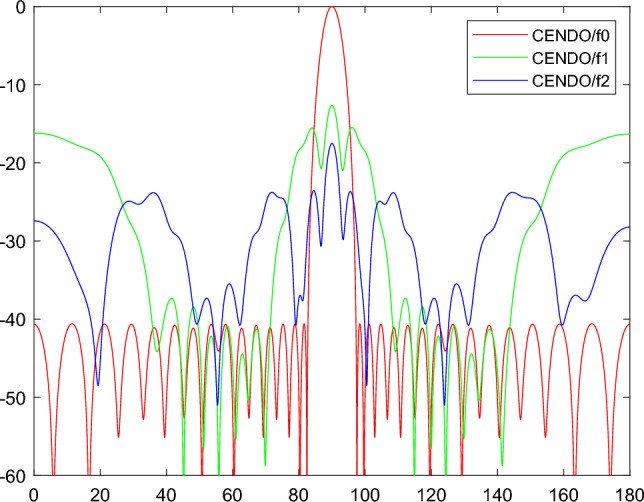
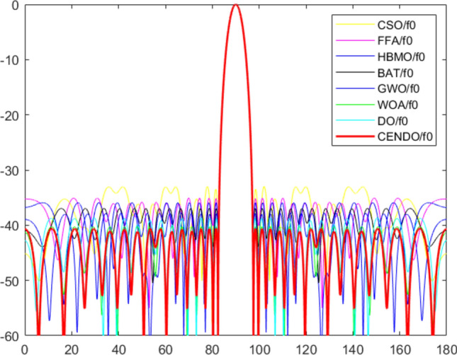
Case-3: this example uses six algorithms, PSO algorithm⁴⁷, real coded genetic algorithm (RGA)⁴⁷, DE algorithm⁴⁷, differential evolution with wavelet mutation (DEWM) algorithm⁴⁷, DO algorithm, and CENDO algorithm, to simulate and optimize an asymmetric 16 element Time-modulation array. The optimal fundamental wave radiation pattern, first harmonic radiation pattern, and second harmonic radiation pattern of different algorithms under this model are obtained, which are shown in Fig. 15, 16a, b, respectively. Table 5 shows the optimal on-time (τ_nn) and optimal uniform spacing (d) of the array elements obtained through different algorithms. Table 6 provides various performance parameter results optimized by different algorithms.

Figure 15.

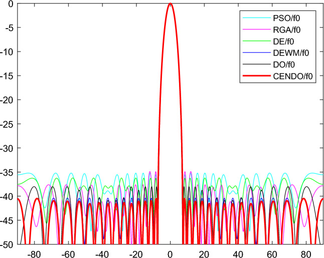
Comparison of fundamental wave radiation patterns using different algorithms.

Figure 16.

Radiation pattern obtained by 6 algorithms: (a) first harmonic, (b) second harmonic.

Table 5.

The optimal on-time and optimal uniform spacing of 16 element arrays obtained by different algorithms.

Algorithms	Optimal on-time (τnn)								Optimal uniform spacing (d)
PSO	0.0900	0.2642	0.3456	0.5186	0.6533	0.8642	0.9426	0.9984	0.8336λ
	0.9892	0.9453	0.8056	0.6587	0.5481	0.3319	0.2256	0.1243
RGA	0.1497	0.2411	0.3701	0.5594	0.6949	0.8491	0.9326	0.9995	0.8151λ
	0.9970	0.9291	0.8031	0.6616	0.5036	0.3627	0.2299	0.1189
DE	0.0946	0.2128	0.3283	0.4896	0.6569	0.7894	0.8892	0.9994	0.8399λ
	0.9807	0.9279	0.8676	0.6826	0.4946	0.3880	0.2183	0.1514
DEWM	0.0875	0.1716	0.2983	0.4442	0.6064	0.7576	0.8831	0.9474	0.8886λ
	0.9586	0.8971	0.7924	0.6454	0.4856	0.3235	0.1919	0.1189
DO	0.1110	0.2079	0.3317	0.4902	0.6571	0.8030	0.9300	0.9985	0.8877λ
	0.9999	0.9500	0.8418	0.6877	0.5275	0.3590	0.2242	0.1370
CENDO	0.0989	0.1853	0.3178	0.4758	0.6541	0.8093	0.9280	0.9988	0.8878λ
	0.9991	0.9359	0.8127	0.6520	0.4881	0.3240	0.1885	0.1043

Significant values are in [bold].

Table 6.

Various performance parameter values of 16 element arrays obtained under 6 algorithms.

Algorithms	PSO	RGA	DE	DEWM	DO	CENDO
SLL (dB)	− 35.21	− 34.89	− 36.23	− 40.41	− 38.03	− 40.50
SBL1 (dB)	− 12.68	− 12.57	− 12.44	− 12.61	− 12.70	− 12.70
SBL2 (dB)	− 17.99	− 17.54	− 17.46	− 17.43	− 17.55	− 17.55
FNBW (deg)	15.12	15.12	15.12	15.12	14.40	15.12
Computational times (s)	~	~	~	~	30.9	30.1

Significant values are in [bold].

The SLL, SBL₁, SBL₂, and FNBW obtained using the CENDO algorithm are − 40.50 dB, − 12.70 dB, − 17.55 dB, and 15.12°, respectively. The PSO algorithm⁴⁷, RGA⁴⁷, DE algorithm⁴⁷, DEWM algorithm⁴⁷, and DO algorithm are used to obtain SLL values of -35.21 dB, -34.89 dB, -36.23 dB, − 40.41 dB, and -38.03 dB, which are 5.29 dB, 5.61 dB, 4.27 dB, 0.09 dB, and 2.47 dB higher than the SLL values obtained by the CENDO algorithm, respectively. For SBL₁, their values reached − 12.68 dB, − 12.57 dB, − 12.44 dB, − 12.61 dB, and -12.70 dB, respectively, which are 0.02 dB, 0.13 dB, 0.26 dB, 0.09 dB, and 0 dB higher than the SBL₁ obtained by the CENDO algorithm. For SBL₂, their values reached − 17.99 dB, − 17.54 dB, − 17.46 dB, − 17.43 dB, and − 17.55 dB, respectively, while the SBL₂ obtained by the CENDO algorithm is 0.01 dB, 0.09 dB, 0.12 dB, and 0 dB lower than that of RGA⁴⁷, DE algorithm⁴⁷, DEWM algorithm⁴⁷, and DO algorithm. For FNBW, the main lobe width of the array obtained by each algorithm is basically around 15°, and the FNBW values obtained by CENDO algorithm, PSO algorithm⁴⁷, RGA⁴⁷, DE algorithm⁴⁷, and DEWM algorithm⁴⁷ are the same, all at 15.12°. So, the concentration of main lobe radiation energy is basically similar, and the directionality of the array is basically the same. For the computational times for algorithm optimization, we can conclude that the computational time for CENDO algorithm optimization of this model is not significantly different from that of DO algorithm and can be approximately equal. Based on the above analysis, the CENDO algorithm shows better results in SLL and SBL compared to other algorithms, therefore, it has strong superiority in pattern synthesis of Time-modulated array.

The optimal opening time (t_on), closing time (t_off), and spacing (d)

Case-4: this example describes a third optimization scheme to reduce the SLL and SBL of TMLA. By combining the optimal opening time (t_on), closing time (t_off), and uniform spacing (d) of each component, the optimal radiation pattern of the Time-modulated array model in this case is obtained. Among them, the excitation amplitude is considered uniform, i.e. I_n = 1, and the comparison algorithms involved include CNEDO algorithm, DO algorithm, PSO algorithm⁴⁸, NPSO algorithm⁴⁸, and NPSOWM algorithm⁴⁸. The population size of each algorithm is set to 100, and the maximum number of iterations is set to 300. Conduct experimental simulation based on the above conditions.

The comparison of the optimal fundamental wave radiation pattern, first harmonic radiation pattern, and second harmonic radiation pattern of NPSOWM⁴⁸, DO, and CENDO algorithms is shown in Figs. 17 and 18a, b, respectively. Table 7 provides the values of SLL, SBL₁, SBL₂, FNBW, and computational times for arrays obtained by different algorithms. The optimal opening time (t_on), closing time (t_off), and optimal uniform spacing (d) of each array element optimized by NPSOWM⁴⁸, DO, and CENDO algorithms are given in Table 8. Figure 19 provides a visual representation of the normalized time series of CENDO algorithm in this case. From the radiation pattern, it can be intuitively seen that the SLL and SBL obtained using the CENDO algorithm are significantly reduced compared to other algorithms. According to the data results in Table 7, regarding the computational times for algorithm optimization, using the DO algorithm to optimize the model takes 76.2 s, while using the CENDO algorithm to optimize the model takes 70.7 s, which is 5.5 s faster than it. Therefore, the CENDO algorithm takes less time and has higher optimization efficiency. The FNBW obtained by optimizing the Time-modulated array model through the above five algorithms is basically the same, with a main lobe width between 14.7° and 14.8°. The use of CENDO algorithm can reduce SLL to -31.72 dB, which is 4.78 dB, 4.13 dB, 0.68 dB, and 0.56 dB lower than the SLL obtained using PSO⁴⁸, NPSO⁴⁸, NPSOWM⁴⁸, and DO algorithms, respectively. The values of SBL₁ and SBL₂ obtained using the CNEDO algorithm are − 19.06 dB and − 21.68 dB, respectively. For SBL₁, the values obtained using the CENDO algorithm are 0.76 dB, 0.81 dB, 0.91 dB, and 0.74 dB lower than those obtained using the PSO⁴⁸, NPSO⁴⁸, NPSOWM⁴⁸, and DO algorithms, respectively; For SBL₂, the values obtained using the CENDO algorithm are 0.46 dB, 0.66 dB, and 0.41 dB lower than those obtained using the NPSO⁴⁸, NPSOWM⁴⁸, and DO algorithms, respectively. To sum up, the results based on the CENDO algorithm are superior to those based on PSO⁴⁸, NPSO⁴⁸, NPSOWM⁴⁸, and DO algorithms in reducing the SLL and SBL of Time-modulated array. This algorithm can better optimize the TMLA model and obtain the desired radiation pattern.

Figure 17.

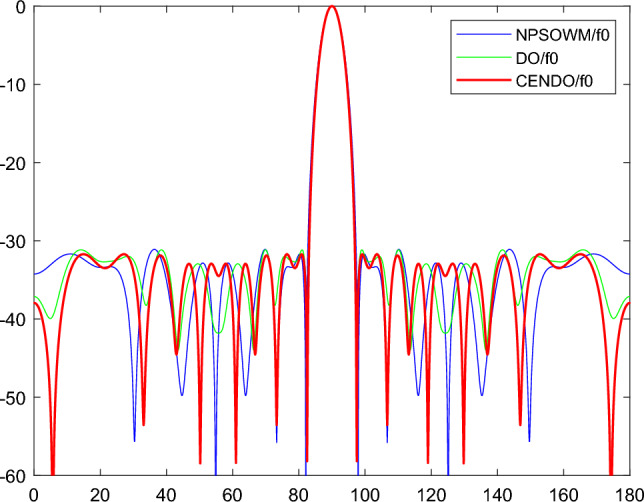
Fundamental wave radiation pattern obtained using NPSOWM, DO, and CENDO algorithms.

Figure 18.

First and second harmonic radiation patterns obtained using NPSOWM, DO, and CENDO algorithms: (a) first harmonic, (b) second harmonic.

Table 7.

Results of array performance parameters obtained using different optimization algorithms for Case-4.

Algorithms	PSO	NPSO	NPSOWM	DO	CENDO
SLL (dB)	− 26.94	− 27.59	− 31.04	− 31.16	− 31.72
SBL1 (dB)	− 18.30	− 18.25	− 18.15	− 18.32	− 19.06
SBL2 (dB)	− 22.00	− 21.22	− 21.02	− 21.27	− 21.68
FNBW (deg)	14.76	14.76	14.76	14.80	14.80
Computational times (s)	~	~	~	76.2	70.7

Significant values are in [bold].

Table 8.

Optimal time series and uniform spacing optimized using NPSOWM, DO, and CENDO algorithms.

Algorithms	Optimal time series (ton and toff)									optimal uniform spacing (d)
NPSOWM	ton	0.92 0.00	0.69 0.00	0.31 0.00	0.00 0.20	0.18 0.00	0.00 0.34	0.00 0.71	0.00 0.94	0.8692λ
	toff	1.00 1.00	0.85 0.92	0.60 0.81	0.42 0.90	0.90 0.39	0.85 0.60	0.94 0.85	1.00 1.00
DO	ton	0.07 0.00	0.02 0.03	0.24 0.13	0.32 0.23	0.03 0.06	0.01 0.64	0.04 0.09	0.00 0.07	0.8876λ
	toff	0.08 1.00	0.17 1.00	0.50 1.00	0.75 0.96	0.75 0.48	0.82 0.96	1.00 0.30	1.00 0.17
CENDO	ton	0.79 0.01	0.01 0.02	0.47 0.01	0.45 0.13	0.01 0.62	0.02 0.46	0.02 0.00	0.00 0.00	0.8888λ
	toff	0.95 1.00	0.18 0.92	0.83 0.87	1.00 0.72	0.79 0.98	0.90 0.74	1.00 0.12	1.00 0.06

Significant values are in [bold].

Figure 19.

Normalized time series graph of 16 element TMLA obtained through CENDO algorithm in Case-4.

Summary

Compared with LAA, TMLA provides a simpler feed network configuration and precisely controls the radiation mode through high-speed RF switches, better achieving ultra-low SLL. This paper introduces an effective design algorithm that simultaneously reduces the SLL and SBL of TMLA, that is, using the CENDO algorithm to design and optimize the time series of TMLA models or a combination of time series and uniform array spacing to achieve the research of TMLA pattern synthesis problem. To objectively analyze and compare the superiority of the algorithms used, this paper compares the CENDO algorithm with different popular evolutionary algorithms such as DE algorithm, PSO algorithm, WOA algorithm, etc. through four simulation examples. They are applied to the optimization design of different Time-modulated array models, and a comprehensive analysis and discussion are conducted from the aspects of radiation pattern, SLL, SBL, and FNBW. The simulation results show that for the above four examples, while keeping the main lobe width unchanged, the radiation pattern of TMLA optimized by the CENDO algorithm with the best time series and the best uniform array spacing has a significant reduction in both SLL and SBL, which verifies that the CENDO algorithm has better optimization performance compared to other optimization algorithms, This also indicates that the CENDO algorithm is an effective method for solving the TMLA pattern synthesis problem. Due to its ability to achieve better optimization characteristics, the CENDO algorithm is expected to be applied in a wide range of other electromagnetic fields.

Author contributions

J.H.L (The first author) proposes the idea and conducts simulation experiments to get the experimental results according to the direction of the research and organizes the data and writes the paper. Y.L (The corresponding author) is mainly responsible for supervising and reviewing papers, including the correctness of research ideas and the standardization of language expression in the manuscript. W.R.Z and T.N.Z (The third and fourth authors) are mainly responsible for checking the charts and data in the paper. Y.B.W and K.H (The fifth and sixth authors) build on the details of the completed paper. All authors reviewed the manuscript.

Funding

This work was supported by National Natural Science Foundation of China (Program No. 62341124), and Yunnan Fundamental Research Projects (Program No.202201AT070030), and the Graduate Research Innovation Fund of Yunnan Normal University (Program No.009002050205502002), and the Scientific Research Fund of Yunnan Provincial Education Department (Program No.2024Y150).

Data availability

All data generated or analyzed during this study are included in this possible article. For the other algorithms in this study, the data were taken from the cited references to compare these data with the results obtained by the CENDO algorithm in this study, and to compare the superior performance of the CENDO algorithm.

Competing interests

The authors declare no competing interests.

References

- 1.Haupt, R. L. Antenna Arrays: A Computational Approach (Wiley, 2010). [Google Scholar]
- 2.Chen, Y., Yang, S. & Nie, Z. Synthesis of uniform amplitude thinned linear phased arrays using the differential evolution algorithm. Electromagnetics27(5), 287–297 (2007). 10.1080/02726340701364233 [DOI] [Google Scholar]
- 3.Panduro, M. A. Design of coherently radiating structures in a linear array geometry using genetic algorithms. AEU-Int. J. Electron. Commun.61(8), 515–520 (2007). 10.1016/j.aeue.2006.09.002 [DOI] [Google Scholar]
- 4.Hansen R C. Contributions of T.T. Taylor to array synthesis. Orlando: Antennas and Propagation Society International Symposium, 1999: 2294–2297.
- 5.Safaai-Jazi, A. A new formulation for the design of Chebyshev arrays. IEEE Trans. Antenn. Propag.42(3), 439–443 (1994). 10.1109/8.280736 [DOI] [Google Scholar]
- 6.Dib, N. I., Goudos, S. K. & Muhsen, H. Application of Taguchi’s optimization method and self-adaptive differential evolution to the synthesis of linear antenna arrays. Progr. Electromagn. Res.102, 159–180 (2010). 10.2528/PIER09122306 [DOI] [Google Scholar]
- 7.Mahouti, P. Design optimization of a pattern reconfigurable microstrip antenna using differential evolution and 3D EM simulation-based neural network model. Int. J. RF Microw. Comput. Aid. Eng.29(8), e21796 (2019). 10.1002/mmce.21796 [DOI] [Google Scholar]
- 8.Recioui, A. Sidelobe level reduction in linear array pattern synthesis using particle swarm optimization. J. Optim. Theor. Appl.153, 497–512 (2012). 10.1007/s10957-011-9953-9 [DOI] [Google Scholar]
- 9.Ghosh, P., Zafar, H. Linear array geometry synthesis with minimum side lobe level and null control using dynamic multi-swarm particle swarm optimizer with local search. Proc. International Conference on Swarm, Evolutionary, and Memetic Computing. Springer, Berlin, Heidelberg, 701–708 (2010).
- 10.Goudos, S. K. et al. Application of a comprehensive learning particle swarm optimizer to unequally spaced linear array synthesis with sidelobe level suppression and null control. IEEE Antenn. Wirel. Propag. Lett.9, 125–129 (2010). 10.1109/LAWP.2010.2044552 [DOI] [Google Scholar]
- 11.Wang, W. B., Feng, Q. & Liu, D. Application of chaotic particle swarm optimization algorithm to pattern synthesis of antenna arrays. Progr. Electromagn. Res.115, 173–189 (2011). 10.2528/PIER11012305 [DOI] [Google Scholar]
- 12.Pappula, L. & Ghosh, D. Linear antenna array synthesis using cat swarm optimization. AEU-Int. J. Electron. Commun.68(6), 540–549 (2014). 10.1016/j.aeue.2013.12.012 [DOI] [Google Scholar]
- 13.Guney, K. & Onay, M. Optimal synthesis of linear antenna arrays using a harmony search algorithm. Exp. Syst. Appl.38(12), 15455–15462 (2011). 10.1016/j.eswa.2011.06.015 [DOI] [Google Scholar]
- 14.Merad, L., Bendimerad, F., Meriah, S. Design of linear antenna arrays for side lobe reduction using the Tabu search method. Int. Arab J. Inf. Technol. (IAJIT), 5(3) (2008).
- 15.Singh, U. & Rattan, M. Design of linear and circular antenna arrays using cuckoo optimization algorithm. Progr. Electromagn. Res. C46, 1–11 (2014). 10.2528/PIERC13110902 [DOI] [Google Scholar]
- 16.Singh, U. & Salgotra, R. Optimal synthesis of linear antenna arrays using modified spider monkey optimization. Arab. J. Sci. Eng.41, 2957–2973 (2016). 10.1007/s13369-016-2053-2 [DOI] [Google Scholar]
- 17.Zaman, M. A. & Abdul Matin, M. Nonuniformly spaced linear antenna array design using firefly algorithm. Int. J. Microw. Sci. Technol.2012(1), 256759 (2012). [Google Scholar]
- 18.Singh, U. & Salgotra, R. Synthesis of linear antenna arrays using enhanced firefly algorithm. Arab. J. Sci. Eng.44, 1961–1976 (2019). 10.1007/s13369-018-3214-2 [DOI] [Google Scholar]
- 19.Singh, U. & Salgotra, R. Synthesis of linear antenna array using flower pollination algorithm. Neural Comput. Appl.29, 435–445 (2018). 10.1007/s00521-016-2457-7 [DOI] [Google Scholar]
- 20.Sun, G. et al. An antenna array sidelobe level reduction approach through invasive weed optimization. Int. J. Ant. Propag.2018, 1–16 (2018). [Google Scholar]
- 21.Saxena, P. & Kothari, A. Optimal pattern synthesis of linear antenna array using grey wolf optimization algorithm. Int. J. Antennas Propag.2016(1), 1205970 (2016). [Google Scholar]
- 22.Kiani, F., Seyyedabbasi, A. & Mahouti, P. Optimal characterization of a microwave transistor using grey wolf algorithms. Analog Integr. Circ. Signal Process.109, 599–609 (2021). 10.1007/s10470-021-01914-y [DOI] [Google Scholar]
- 23.Zhu, Q. et al. A pattern synthesis approach in four-dimensional antenna arrays with practical element models. J. Electromagn. Waves Appl.25(16), 2274–2286 (2011). 10.1163/156939311798147105 [DOI] [Google Scholar]
- 24.Chen, Y., Yang, S. & Nie, Z. Improving conflicting specifications of time-modulated antenna arrays by using a multiobjective evolutionary algorithm. Int. J. Numer. Modell. Electron. Netw. Dev. Fields25(3), 205–215 (2012). 10.1002/jnm.824 [DOI] [Google Scholar]
- 25.Chakraborty, A., Ram, G. & Mandal, D. Pattern synthesis of timed antenna array with the exploitation and suppression of harmonic radiation. Int. J. Commun. Syst.34(4), e4727 (2021). 10.1002/dac.4727 [DOI] [Google Scholar]
- 26.Tennant, A. & Chambers, B. A two-element time-modulated array with direction-finding properties. IEEE Antenn. Wirel. Propag. Lett.6, 64–65 (2007). 10.1109/LAWP.2007.891953 [DOI] [Google Scholar]
- 27.Li, G., Yang, S. & Nie, Z. Direction of arrival estimation in time modulated linear arrays with unidirectional phase center motion. IEEE Trans. Antenn. Propag.58(4), 1105–1111 (2010). 10.1109/TAP.2010.2041313 [DOI] [Google Scholar]
- 28.Chakraborty, A., Ram, G. & Mandal, D. Time-modulated multibeam steered antenna array synthesis with optimally designed switching sequence. Int. J. Commun. Syst.34(9), e4828 (2021). 10.1002/dac.4828 [DOI] [Google Scholar]
- 29.Chakraborty, A., Ram, G., Mandal, D. Electronic beam steering in timed antenna Array by controlling the harmonic patterns with optimally derived pulse-shifted switching sequence. Proc. International Conference on Innovative Computing and Communications: Proceedings of ICICC 2021, Vol 3. Springer Singapore, 205–216 (2022).
- 30.Hardel, G. R., Yallaparagada, N. T,, Mandal, D., et al. Introducing deeper nulls for time modulated linear symmetric antenna array using real coded genetic algorithm. Proc. 2011 IEEE Symposium on Computers & Informatics. IEEE, 249–254 (2011).
- 31.Yang, S., Gan, Y. B. & Qing, A. Sideband suppression in time-modulated linear arrays by the differential evolution algorithm. IEEE Antenn. Wirel. Propag. Lett.1, 173–175 (2002). 10.1109/LAWP.2002.807789 [DOI] [Google Scholar]
- 32.Yang, S. et al. Design of a uniform amplitude time modulated linear array with optimized time sequences. IEEE Trans. Antenn. Propag.53(7), 2337–2339 (2005). 10.1109/TAP.2005.850765 [DOI] [Google Scholar]
- 33.Li, G. et al. Sidelobe suppression in time modulated linear arrays with unequal element spacing. J. Electromagn. Waves Appl.24(5–6), 775–783 (2010). 10.1163/156939310791036368 [DOI] [Google Scholar]
- 34.Mandal, D., Yallaparagada, N. T,, Ghoshal, S. P., et al. Wide null control of linear antenna arrays using particle swarm optimization. Proc. 2010 Annual IEEE India Conference (INDICON). IEEE, 1–4 (2010).
- 35.Rocca, P., Oliveri, G. & Massa, A. Differential evolution as applied to electromagnetics. IEEE Antenn. Propag. Magaz.53(1), 38–49 (2011). 10.1109/MAP.2011.5773566 [DOI] [Google Scholar]
- 36.Zhao, S. et al. Dandelion optimizer: A nature-inspired metaheuristic algorithm for engineering applications. Eng. Appl. Artif. Intell.114, 105075 (2022). 10.1016/j.engappai.2022.105075 [DOI] [Google Scholar]
- 37.Persohn, K. J. & Povinelli, R. J. Analyzing logistic map pseudorandom number generators for periodicity induced by finite precision floating-point representation. Chaos Solitons Fractals45(3), 238–245 (2012). 10.1016/j.chaos.2011.12.006 [DOI] [Google Scholar]
- 38.Nezhad, S. Y. D., Safdarian, N. & Zadeh, S. A. H. New method for fingerprint images encryption using DNA sequence and chaotic tent map. Optik224, 165661 (2020). 10.1016/j.ijleo.2020.165661 [DOI] [Google Scholar]
- 39.Lawnik, M. Combined logistic and tent map. J. Phys. Conf. Ser.1141(1), 012132 (2018). 10.1088/1742-6596/1141/1/012132 [DOI] [Google Scholar]
- 40.Einstein, A. Investigations on the Theory of the Brownian Movement (Courier Corporation, 1956). [Google Scholar]
- 41.Mantegna, R. N. Fast, accurate algorithm for numerical simulation of Levy stable stochastic processes. Phys. Rev. E49(5), 4677 (1994). 10.1103/PhysRevE.49.4677 [DOI] [PubMed] [Google Scholar]
- 42.Bregains, J. C. et al. Signal radiation and power losses of time-modulated arrays. IEEE Trans. Antenn. Propag.56(6), 1799–1804 (2008). 10.1109/TAP.2008.923345 [DOI] [Google Scholar]
- 43.Chakraborty, A., Ram, G. & Mandal, D. Optimal pulse shifting in timed antenna array for simultaneous reduction of sidelobe and sideband level. IEEE Access8, 131063–131075 (2020). 10.1109/ACCESS.2020.3010047 [DOI] [Google Scholar]
- 44.Zhu, Q. et al. Design of a low sidelobe time modulated linear array with uniform amplitude and sub-sectional optimized time steps. IEEE Trans. Antenn. Propag.60(9), 4436–4439 (2012). 10.1109/TAP.2012.2207082 [DOI] [Google Scholar]
- 45.Patra, S., Mandal, S. K., Mahanti, G. K. et al. Linear and non-linear synthesis of unequally spaced time-modulated linear arrays using evolutionary algorithms. Radioengineering, 30(3) (2021).
- 46.Poddar, S. et al. Design optimization of linear arrays and time-modulated antenna arrays using meta-heuristics approach. Int. J. Numer. Modell. Electron. Netw. Dev. Fields35(5), e3010 (2022). 10.1002/jnm.3010 [DOI] [Google Scholar]
- 47.Ram, G. et al. Directivity maximization and optimal far-field pattern of time modulated linear antenna arrays using evolutionary algorithms. AEU-Int. J. Electron. Commun.69(12), 1800–1809 (2015). 10.1016/j.aeue.2015.09.009 [DOI] [Google Scholar]
- 48.Chakraborty, A., Ram, G. & Mandal, D. Time-modulated linear array synthesis with optimal time schemes for the simultaneous suppression of sidelobe and sidebands. Int. J. Microwav. Wirel. Technol.14(6), 768–780 (2022). 10.1017/S175907872100088X [DOI] [Google Scholar]
Associated Data
This section collects any data citations, data availability statements, or supplementary materials included in this article.
Data Availability Statement