

Abstract
Peripheral Capillary Oxygen Saturation (SpO2) has received increasing attention during the COVID-19 pandemic. Clinical investigations have demonstrated that individuals afflicted with COVID-19 exhibit notably reduced levels of SpO2 before the deterioration of their health status. To cost-effectively enable individuals to monitor their SpO2, this paper proposes a novel neural network model named “ITSCAN” based on Temporal Shift Module. Benefiting from the widespread use of smartphones, this model can assess an individual’s SpO2 in real time, utilizing standard facial video footage, with a temporal granularity of seconds. The model is interweaved by two distinct branches: the motion branch, responsible for extracting spatiotemporal data features and the appearance branch, focusing on the correlation between feature channels and the location information of feature map using coordinate attention mechanisms. Accordingly, the SpO2 estimator generates the corresponding SpO2 value. This paper summarizes for the first time 5 loss functions commonly used in the SpO2 estimation model. Subsequently, a novel loss function has been contributed through the examination of various combinations and careful selection of hyperparameters. Comprehensive ablation experiments analyze the independent impact of each module on the overall model performance. Finally, the experimental results based on the public dataset (VIPL-HR) show that our model has obvious advantages in MAE (1.10%) and RMSE (1.19%) compared with related work, which implies more accuracy of the proposed method to contribute to public health.
Keywords: SpO2 estimation, Temporal shift convolution, Imaging PhotoPlethysMography, ITSCAN
Subject terms: Computational biology and bioinformatics, Mathematics and computing
Introduction
SpO2 is an important indicator to reflect the human cardiovascular and cerebrovascular function for clinical medical monitoring1. In addition, many lung diseases can be detected early by monitoring abnormal values of SpO2. For example, it has been reported that some COVID-19 patients did not show respiratory symptoms, only clinically significant hypoxemia2. Thus, timely detection of changes in SpO2 is of great essential to the protection of life and health. Conventional SpO2 detection methods can be divided into two types: arterial blood gas (ABG) analysis3 and photoplethysmography (PPG)4. ABG needs to collect blood from the human body first and measure the SpO2 partial pressure through electrochemical analysis to obtain the SpO2 saturation. PPG generally uses a finger-clip photoelectric sensor to calculate the SpO2 saturation by measuring the reflected light intensity of two incident light sources with different wavelengths, such as the red light wavelength (660–700 nm) and the infrared (IR) light wavelength (800–950 nm)5. Both methods belong to the contact measurement ways, which suggests they are not suitable for patients requiring non-contact monitoring even for skin damage. To achieve user-friendly non-contact measurements, Imaging PhotoPlethysMography (IPPG) is widely used due to its advantages of capturing physiological measurements with digital cameras and ambient light6.
There have been some studies on the relationship between IPPG and SpO2, but lots of them are still in their infancy. The Radio of Radios method (ROR) by regression is a commonly used method to predict SpO2, which transitions the range of datasets from the infrared to the visible domain. For example, Kong et al. use a band-pass filter to lock red and green channels as input variables, and predict SpO2 without introducing additional light sources7; Al-Naji et al. introduce complete Ensemble Empirical Mode Decomposition (EEMD) and Independent Component Analysis (ICA) to extract the features of facial video as the input of ROR to predict SpO28; Sun et al. improve the ROR algorithm and uses Multiple Linear Regression (MLR) to extract red and blue channel for predicting SpO29; Luo et al. design a special sampling device based on the facial video to obtain more comprehensive ROR input variables10; Rosa et al. utilize Eulerian Video Magnification (EVM) to preprocess facial video to amplify changes in reflected light for more sensitive input variables11. Shao et al.12 preset the ROR standard model to align individuals with the standard model. Hamoud et al.13 innovatively used XGBoost Regression to achieve SPO2 measurement based on ROR. Chan et al.14 applied the ROR for two combinations to access the accuracy under four lighting conditions. The main innovations of researchers using conventional methods are reflected in the preprocessing of data, while there are few algorithm innovations for predicting SpO2. Another commonly used method for predicting SpO2 is called the Pulse Blood Volume (PBV) method15. Unlike ROR, which needs to capture the DC and AC components of two different exact wavelengths of visible light, PBV utilizes the different relative pulsatile amplitudes in the color channels to distinguish changes in blood volume caused by SpO2. For example, Van Gastel et al. proposed an Adaptive PBV method (APBV) for BVP signals extraction from multiple ROIs, followed by their mapping to different SpO2 levels ranging from 65 to 100% with an interval of 5%16. Although PBV is simpler in terms of data processing, this comes at the cost of reduced accuracy. Moreover, the above two conventional methods have poor anti-interference ability and have extremely high requirements for the quality of the datasets.
With the rapid development of machine learning, especially deep neural network, a rapidly increasing number of researchers have applied them to biomedical scenarios and daily health monitoring. In particular, deep learning techniques have matured in predicting HRV metrics17, so deep learning algorithm is also used for the contactless SpO2 measurement. Zheng18 proposed a hybrid model, which has a mixed network architecture consisting of CNN, convolutional long short-term memory (convLSTM), and video vision transformer (ViViT). Peng et al.19 proposed a contrastive learning spatiotemporal attention network, an innovative semi-supervised network for video-based SpO2 estimation. Cheng et al.20 used the spatial temporal representation to record features and CNN consisted with EfficientNet-B3 to predict SpO2 value. Mathew et al.21 first propose the convolutional neural network based on a noncontact SpO2 estimation scheme using a smartphone camera. This paper compares the influence of the sequence of processing temporal features and spatial features on the SpO2 estimation results and finally concludes that processing the two features at the same time has the smallest Mean Absolute Error (MAE) and Root Mean Square Error (RMSE). However, without an attention mechanism, model training cannot focus on skin pixels, causing serious interference from environmental noise and low robustness. Yusuke et al. decompose the input video into direct current (DC) and alternating current (AC) components using a filter. These components are subsequently input into ResNet18 separately, and the SpO2 value is ultimately derived through a fully connected layer22.
Nevertheless, they use a self-sampled dataset, lacking comparisons with other researchers, and the structure of directly outputting SpO2 using a fully connected layer is open to debate. Casalino et al.23 overcame one of the main issues of non-contact SpO2 measurement based on pure data sets, which is the frequent change of perspective viewpoint due to head movements, which makes it more difficult to identify the face and measure SpO2. Verkruysse et al.24 used two public datasets (rPPG datasets and BIDMC datasets) to extract multimodal physiological information including SpO2. In model architecture, Researchers have undertaken numerous efforts. Hu et al.25 first introduced Residual and Coordinate Attention (RCA) into the SpO2 estimation module as feature extraction network. This paper constructs a Color Channel Model (CCM) based on an image generator and a Network-Based Model (NBM), finally combining the two into the Multi-Model Fusion Model (MMFM), which achieves the optimal solution. Nonetheless, the researchers solely took into account the spatial features of facial videos, neglecting the spatiotemporal features of SpO2. Empirical investigations have conclusively demonstrated that the sequence in which temporal and spatial features are extracted exerts a discernible influence on the accuracy of SpO2 prediction21. It is imperative to attain concurrent extraction of both temporal and spatial features to optimize predictive performance. From the evaluation metrics, Bal26 observed the Pearson correlations by comparing the Pearson coefficient between our SpO2 estimations and the commercial oximeter readings. Stogiannopoulos et al.27 used the RMSE and Pearson to estimating SpO2 values. Verkruysse et al.28 used the MAE to evaluate, which was validated in controlled conditions for an SpO2 range of 83–100%. Pirzada29 used the ROR method for measurement, but the metrics was also RMSE between the estimated SpO2 and the real value. Avram et al.30 explained the quality of the work by judging whether the RMSE result exceeds the FDA-recognized ISO 81060-2-61:2017 standard.
Inspired by the contactless Heart Rate (HR) estimation using IPPG31, this paper utilizes the Improved Temporal Shift Convolutional Attention Network (ITSCAN) for SpO2 estimation for the first time. In light of the prevailing challenges encountered in contemporary SpO2 estimation tasks, several noteworthy issues merit consideration:
Inadequate Feature Extraction Methodology The current models in use exhibit limitations in feature extraction as they do not concurrently account for temporal and spatial characteristics. Moreover, they lack an attention mechanism, precluding the capacity to selectively focus on skin pixels of utmost relevance. Additionally, the output generated via the fully connected layers lacks interpretability, impeding the model’s transparency and the ability to discern the basis for predictions.
Lack of Rigorous Loss Function Selection A second pertinent concern pertains to the absence of a systematic approach in the selection of appropriate loss functions for the SpO2 estimation task. This omission has profound implications for the model’s performance and convergence properties. An in-depth analysis and rationale for the chosen loss functions are warranted to ensure their alignment with the specific characteristics of the problem at hand, as well as to optimize training dynamics.
Limited Dataset Utilization and Reproducibility Concerns A third salient issue revolves around the predominant reliance on self-built datasets by most researchers within the field. This practice raises concerns regarding the generalizability of findings and the robustness of experimental outcomes.
In response to the aforementioned challenges, this paper makes the following substantial contributions:
We propose a novel deep learning model architecture for SpO2 estimation, which is consists of two distinct branches, seamlessly interconnected via a coordinate attention mechanism. The model introduces TSM to extract spatiotemporal features, employs Residual Network to capture pertinent facial skin pixels, combines skin pixel positions with feature maps through coordinate attention, and finally deploys a specialized SpO2 Estimator in lieu of conventional fully connected layer for more robust estimation.
In a pioneering effort, we consolidate prevalent loss functions commonly employed in SpO2 estimation tasks. Subsequently, we conduct comprehensive comparative experiments to discern optimal combinations of these loss functions that best align with our model. Significantly, we introduce a novel composite loss function encompassing the Negative Pearson coefficient (NegPearson) and SmoothL1 for the precise estimation of SpO2 value.
To facilitate comparison with the related work, we conduct rigorous experimentation on public datasets (VIPL-HR) and compare the results with traditional methods and contemporary deep learning methods in recent literature. Judging from the results, the proposed method out perms in all aspects, especially in RMSE which shows significant advantages.
Methods
Datasets
In the current research on contactless SpO2 estimation, most researchers use self-built datasets instead of public ones, and most of them have fewer subjects and scenes. The experiments in this paper are conducted on the public datasets of VIPL-HR for easier comparison and more convincing32. The VIPL-HR database contains 9 scenarios for 107 subjects recorded by 4 different devices, which note the HR, SpO2, and Blood Volume Pulse (BVP) signal of each video at the same time.
In order to verify the running status of the algorithm on devices with poor performance, this paper selects SOURCE1, in which the video is recorded by a Logitech C310 web camera with 25 frames and a resolution of , as the dataset. 80% of the data was used as the training set, 10% as the validation set, and 10% as the test set. The SpO2 starts recording at the same time as the video, and a SpO2 value is recorded every second. The histogram of the SpO2 value distribution of the data set is shown in Fig. 1. The range of SpO2 from VIPL-HR is 84 to 99.
Figure 1.

The histogram of label distribution of the dataset VIPL-HR, and label is SpO2 level.
Traditional method
According to the literature33, SpO2 is the percentage of oxygenated hemoglobin in peripheral capillaries, which can be expressed as Eq. (1).
| 1 |
where is the concentration of deoxygenated hemoglobin and is the concentration of oxygenated hemoglobin. The Beer–Lambert Law states the light absorption by a substance in a solution is proportional to its concentration34. Set the light intensity incident on the tissue as . After passing through human tissue, the intensity of transmitted light can be expressed as Eq. (2).
| 2 |
where , , represent the total extinction coefficient of non-pulsatile components in tissue and venous blood, the concentration of light-absorbing substances, and distance travelled by light in tissue, respectively. The and represent the extinction coefficient of deoxygenated hemoglobin and the extinction coefficient of oxygenated hemoglobin. The represents the distance travelled by light in arterial blood. Then, the absorbance of human tissue can be defined as Eq. (3).
| 3 |
As the human heart beats, the light intensity of light penetrating arteries will reach the minimum and maximum, and the absorbance of human tissue fluctuates between maximum and minimum values. Obviously, can be cancelled by the max and the min , which means the influence of blood tissue can be eliminated by changes in light absorption caused by blood volume fluctuations. It is shown in Eq. (4).
| 4 |
where , represent the DC component and the AC component, respectively. represents the difference of the distance travelled by light. For the same subject, is the same at different wavelengths. Obviously, in the scene of two different wavelengths of light, the influence can be eliminated, which is shown in Eq. (5).
| 5 |
where and represent the different wavelengths, and represents the radio of the AC component and the DC component. Combined with Eqs. (1) and (5), we can rewrite the calculation model as Eq. (6).
| 6 |
According to the optical absorption spectra of HbO2 and Hb shown in Fig. 2, when the absorption of Hb and HbO2 of light of wavelength is equal, Eq. (6) can be written as Eq. (7).
| 7 |
Figure 2.

Absorption spectrum of HbO2 and Hb10.
Therefore, the red light with a wavelength of 660 nm is usually referred to as . In the visible light range, light with wavelengths of 440 nm and 520 nm is usually used as . For each subject, this paper gets its BVP signal by video, and then calculates the average peak-to-peak and average values of the BVP signals of different color channels as AC and DC components respectively, and finally fits the SpO2 curve.
Another traditional method PBV is not discussed in this paper because it can only roughly calculate SpO2.
Deep learning method ITSCAN
The proposed SpO2 estimation model based on deep learning is shown in Fig. 3, which consists of a motion branch and an appearance branch. And the identifiable image in Fig. 3 is taken from a dataset, named VIPL-HR. The appearance branch is responsible for capturing the detailed features of the face in the video by the Residual Network, and introducing it into the motion branch through the attention mechanism. The motion branch uses Temporal Shift Module (TSM)35 instead of 3D Convolution Neural Network (3DCNN) to extract spatial–temporal features, which helps to reduce calculation time. Different from TSCAN’s frame-by-frame estimation of HR, ITSCAN’s motion branch introduces a SpO2 Estimator at the end to map the features learned by the model into a separate SpO2, realizing second-by-second SpO2 prediction. By doing so, ITSCAN not only significantly reduces computational time by only calculating the attention mask once, but also captures most of the pixels that contain skin and reduces camera quantization error. ITSCAN is derived from MTTS-CAN, but they exhibit distinct differences in task types, application scenarios, and model architectures. MTTS-CAN. MTTS-CAN is used to measure HR and Resp by introducing self-attention masks twice in regression tasks, while ITSCAN is used to measure SpO2 by introducing coordinate attention, residual network and SpO2 estimator in classification.
Figure 3.

Overview of the ITSCAN model.
TSM network
This section introduces a TSM Network to extract features with physiological information from face videos and uses them to calculate the SpO2. The TSM Network is shown in Fig. 4.
Figure 4.
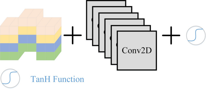
The TSM network module operates by using frame dislocation and 2D CNN to achieve synchronous extraction of spatiotemporal features.
2D CNN is widely used to extract image features, but IPPG needs to extract more complex spatiotemporal features. Therefore, 3D CNN, which can better take into account spatiotemporal features, is used for video processing. However, there is still a problem with 3D CNN because it needs to process temporal and spatial features at the same time, resulting in a large computational overhead. While 2D CNN can guarantee computational efficiency but cannot effectively extract temporal features. TSM is naturally proposed as a compromise between 3D CNN and 2D CNN, the schematic diagram of which is shown in Fig. 5.
Figure 5.

The schematic diagram of TSM specific operations.
In this paper, the total number of channels is divided by 3, 1/3 of the channels shift forward along the temporal axis, the other 1/3 shifts backward along the temporal axis, and the remaining 1/3 channels are unchanged. When some channel shifting exceeds the theoretical time length, the excess frames are truncated and the empty part is filled with zero. TSM realizes the exchange of spatial information between different frames so that the subsequent 2D CNN operation can extract spatial features including other time dimensions. Moreover, the operations of truncation and zero padding also ensure the invariance of the original time sequence.
The coordinate attention
Affected by the environment, large amplitude head movements and light conditions will affect the extraction of facial features, resulting in distortion of SpO2 estimation36. Meanwhile, to minimize the negative effects introduced by shifting tensor, an attention module is inserted in ITSCAN. The coordinated attention mechanism performs convolution, normalization, pooling, and activation operations on the horizontal and vertical features information of the image, realizing the integration of spatial coordinate information and constructing a coordinate-aware attention map. In the paper, the coordinate attention module is embedded into the appearance branch, and the network structure is shown in Fig. 6.
Figure 6.

The coordinate attention module structure first extracts the height and width features of the input data independently, and then learns them comprehensively.
The input can be expressed as . Through the average pooling layer, the input is encoded separately in the horizontal and vertical directions, allowing the attention module to capture the precise location of facial features. Thus, the output of the c-th channel at width can be written as Eq. (8), and the output of the c-th channel at height can be written as Eq. (9).
| 8 |
| 9 |
and represent the height and width of the image respectively. The size of the horizontal feature map is and the size of the vector feature map is . Both are merged into a new feature map, the size of which is . The results are passed through the convolution layer, normalization layer and activation layer respectively.
Then, the features are evenly divided into part and according to the second dimension, and then sent to the convolution layer respectively, so that their dimensions are again consistent with the dimensions of the input features of the coordinate attention module. Finally, the output is denoted by Eq. (10).
| 10 |
Residual network
The paper refers to the literature25 to construct a residual network for feature extraction as shown in Fig. 7. In the residual network, the introduction of jump links greatly alleviates the vanishing gradient problem. At the same time, directly connecting the input features to the output via a bypass reduces information loss and further improves network performance. After experimental testing, when the number of residual blocks is 2, the residual network has the best effect.
Figure 7.

Specific architecture of the module Residual Network, which includes two layers of Residual Block.
SpO2 estimator
The SpO2 Estimator is shown in Fig. 8. It maps the high-dimensional features to SpO2 corresponding to time. Since SpO2 can equal interval discrete values from 1 to 100%, i.e., the sequential vector . The channels of input are compressed to 100 by a convolution layer, consisting with . Subsequently, obtain the feature map with these 100 channels by a normalization layer and a Softmax activation layer.
Figure 8.
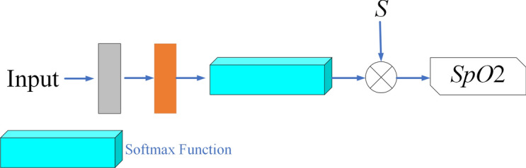
Specific architecture of the SpO2 estimator. Map the input features to SpO2 value through the softmax function.
The loss function
In the SpO2 estimation task, the MAE and RMSE between the predicted result and the real result are the targets that researchers care about. According to NBR ISO 80601-2-61:2015, to validate equipment for SpO2 estimation, the RMSE value must be less than 2% of the declared range11. MAE is also the smaller the better. At the same time, if the change trend of the estimated SpO2 is basically consistent with the actual value, it means that the estimated SpO2 can reflect the real situation. So, The Pearson coefficient is naturally also used to evaluate the quality of prediction results. The formulas are defined from Eqs. (11) to (13).
| 11 |
| 12 |
| 13 |
where T is the length of the SpO2 array, X is the gold standard SpO2 series, and Y is the estimated SpO2 series.
In predicting the SpO2 task using deep neural networks, there are a total of 5 loss functions that are commonly used, namely MSE22, RMSE21, SmoothL125, NegPearson22, and cross entropy25. The SmoothL1, NegPearson, and Cross Entropy are defined from Eqs. (14) to (16). The paper compares the effectiveness of new loss functions formed by linear combinations of the above 5 loss functions in predicting SpO2. Finally, it was concluded that the combination of SmoothL1 and NegPearson has the best results. Specific experimental results are displayed in Experiments.
| 14 |
| 15 |
| 16 |
where T is the length of the SpO2 array, X is the gold standard SpO2, and Y is the estimated SpO2. represents the probability that the gold standard SpO2 at time i is estimated to be j, and represents the probability that the estimated SpO2 at time i is estimated to be j.
Results and discussion
Experiment setting
In preprocessing, the original video is segmented into groups of 25 frames because each 25 frames represent one piece of recorded SpO2. Use the OpenCV open haarcascade_frontalface_default.xml file to locate the position of the face part in the video. Moreover, to avoid missed detection, the height and width of the recognition anchor frame are multiplied by 1.5 times. In the process of model training, the AdamW decay approach is implemented, with a learning rate of 1e−4. Each training iteration consists of 20 epochs and is conducted on a dual setup of GeForce RTX 2080 Ti GPUs.
Considering that there are two branches in the model, the original video image is processed in two different normalization ways. The image input to the motion branch is firstly subjected to difference operation and then normalized, and the image input to the appearance branch is only normalized. During normalization, this paper compresses each frame image to the same standard size. Therefore, this paper compares the ITSCAN model performance under different input image sizes. This paper summarizes the commonly used loss functions for predicting SpO2, and linearly combines them to select the loss function with the best results. Likewise, this paper uses ablation experiments to verify the impact of each module on the prediction results. In conclusion, this paper conducts a comprehensive comparative analysis, aligning its findings with those of contemporaneous researchers. In all tables, all values are average values, and the bold values indicate minimal or maximum errors. This paper uses MAE, RMSE, and Pearson coefficients to evaluate the experimental results. Example test prediction curves are shown for reference in Fig. 9.
Figure 9.

Prediction curves under different circumstances.
Where the blue line represents the individual’s actual SpO2 and the red line represents the predicted SpO2 by ITSCAN.
Results and discussion
Image size
To verify the impact of different input image sizes on the experimental results, the facial areas are segmented from the original image using a rectangular anchor frame and resized to various sizes. Table 1 presents the prediction results under different input image sizes, which is the optimal loss function at this time.
Table 1.
Comparative experimentation of image sizes.
| Image size | MAE (%) | RMSE (%) | Pearson |
|---|---|---|---|
| 64 × 64 | 1.28 | 1.29 | 0.355 |
| 128 × 128 | 1.37 | 1.50 | 0.312 |
| 256 × 256 | 1.10 | 1.19 | 0.375 |
| 320 × 320 | 1.32 | 1.39 | 0.343 |
| 400 × 400 | 1.31 | 1.38 | 0.302 |
According to Table 1, increasing the pixel size of images can indeed obtain more texture and contextual information, which is beneficial to capture better features. In addition, it is easier to obtain discriminative features when images become large. On the one hand, the utilization of excessively large input images results in an increase in model size and complexity, which can lead to overfitting. On the other hand, this approach is susceptible to introducing superfluous features that may subsequently reduce the model’s predictive accuracy. From the experiment, the input image size is set to , which is more suitable.
A comprehensive investigation into the influence of input image dimensions on model performance within the context of the PURE dataset is conducted25. Specifically, the study evaluated 7 distinct image sizes, namely 32, 112, 196, 224, 304, 352, and 448 pixels. The findings demonstrated that the employment of the pixel image dimensions yielded the most favorable outcomes in terms of model performance, which is match with our experiment ().
Time length
To examine the effect of input data over varying time lengths on model performance, this paper evaluates the model using input data at different time scales. Since the video frame rate of VIPL-HR is 25 fps, the length of the input data is an integer multiple of 25 frames. Table 2 presents the prediction results under different input time length, which is the optimal loss function at this time.
Table 2.
Comparative experimentation of time length.
| Time length (s) | MAE (%) | RMSE (%) | Pearson |
|---|---|---|---|
| 1 | 1.10 | 1.19 | 0.375 |
| 2 | 1.03 | 1.21 | 0.368 |
| 3 | 1.35 | 1.44 | 0.351 |
| 5 | 1.37 | 1.41 | 0.321 |
According to Table 2, as the length of input data increases, the overall model performance exhibits a downward trend. This phenomenon may be attributed to the excessive amount of input data combined with the minimal variation in SpO2 as a label, which hinders the model’s ability to effectively learn features. However, the MAE indicator slightly improves from the 1 to 2-s time scale, indicating that the model retains a certain level of processing capability for 2-s length data. In summary, the model proposed in this paper achieves SpO2 evaluation within seconds.
Loss function
A suitable loss function helps the model adapt to the data. This paper evaluates the performance of several commonly used loss functions in SpO2 prediction tasks. The results are shown in Table 3. For convenience of expression, MSE is denoted as M, RMSE is denoted as R, SmoothL1 is denoted as S, CrossEntropy is denoted as C, and NegPearson is denoted as N. At this juncture, the weights associated with the components of the linear combination within the loss function are equitably set.
Table 3.
Comparative experimentation of loss functions.
| Loss Function | MAE (%) | RMSE (%) | Pearson | Loss function | MAE (%) | RMSE (%) | Pearson |
|---|---|---|---|---|---|---|---|
| MSE | 1.88 | 1.99 | 0.304 | M + R + S | 1.42 | 1.50 | 0.294 |
| RMSE | 1.64 | 1.74 | 0.313 | M + R + N | 1.46 | 1.54 | 0.274 |
| SmoothL1 | 1.43 | 1.51 | 0.281 | M + R + C | 1.98 | 2.09 | 0.211 |
| NegPearson | 5.55 | 5.63 | 0.329 | M + S + N | 1.46 | 1.54 | 0.336 |
| Cross Entropy | 2.14 | 2.24 | Nan | M + S + C | 2.00 | 2.11 | 0.295 |
| M + R | 1.46 | 1.55 | 0.291 | M + N + C | 1.59 | 1.69 | 0.247 |
| M + S | 1.35 | 1.43 | 0.324 | R + S + N | 1.88 | 1.98 | 0.287 |
| M + N | 1.43 | 1.51 | 0.290 | R + S + C | 1.72 | 1.82 | 0.289 |
| M + C | 1.46 | 1.54 | 0.286 | R + N + C | 2.01 | 2.11 | 0.238 |
| R + S | 1.39 | 1.47 | 0.275 | S + N + C | 2.07 | 2.18 | 0.210 |
| R + N | 1.49 | 1.58 | 0.194 | M + R + S + N | 1.46 | 1.54 | 0.303 |
| R + C | 1.58 | 1.68 | 0.235 | M + R + S + C | 2.07 | 2.18 | 0.294 |
| S + N | 1.46 | 1.56 | 0.318 | M + S + N + C | 1.59 | 1.79 | 0.228 |
| S + C | 1.59 | 1.69 | 0.245 | R + S + N + C | 1.79 | 1.89 | 0.275 |
| N + C | 4.39 | 4.39 | 0.214 | ALL | 1.51 | 1.61 | 0.301 |
According to Table 3, bold fonts represent the best results, and the results exceeding 0.3 in the Pearson coefficient are highlighted in italics font. It is evident that selecting M and S as the loss functions leads to the attainment of minimum values for MAE and RMSE, respectively. Meanwhile, loss functions associated with green font consistently incorporate combinations of M, S, or N. Despite the fact that utilizing the sole loss function S results in a Pearson coefficient of only 0.281, substantial enhancements in both MAE and RMSE are evident. Therefore, this does not preclude the inclusion of S in the subsequent discussion within this article. Choosing the simplest possible loss function can reduce the space complexity of model calculation. Consequently, when indicators of M + S and M + N + S are not much different, it is best to use M + S as the ITSCAN model loss function. Based on this idea, this paper considers pairwise combinations of M, N, and S to explore the optimal combination weight. The results are shown in Fig. 10.
Figure 10.

The impact of hyperparameters on model results under the combination of three different loss functions.
Absolutely, in the case where the combination of the SmoothL1 and NegPearson loss functions is employed (), MAE attains its minimum value (), while RMSE reaches its minimum value (). Additionally, the Pearson correlation coefficient achieves its maximum value under this configuration ().
Ablation experiment
The ITSCAN model introduces a total of four modules, namely the TSM Network, Coordinate attention network, Residual network and SpO2 estimator. To verify the impact of each network on the overall ITSCAN and thus illustrate the necessity of adding these modules, this paper conducts ablation experiments by replacing modules one by one.
Use ordinary 2D convolutional layers instead of a Residual network to extract facial features. Only the convolution operation is performed between the TSM network output and the appearance branch output instead of the coordinate attention network. Remove the TSM network architecture and exclusively employ convolutional layers for feature extraction. Replace the SpO2 estimation network with a fully connected layer. The ablation experiment results are shown in Table 4.
Table 4.
Comparative experimentation of model modules.
| MAE (%) | RMSE (%) | Pearson | |
|---|---|---|---|
| ITSCAN without a TSM network | 1.42 | 1.51 | 0.281 |
| ITSCAN without Residual network | 1.71 | 1.81 | 0.343 |
| ITSCAN without Coordinate attention | 1.95 | 2.05 | 0.243 |
| ITSCAN without SpO2 estimator | 2.70 | 2.87 | 0.319 |
| ITSCAN | 1.10 | 1.19 | 0.375 |
It is evident that in the absence of the SpO2 estimator incorporation, the predicted SpO2 values exhibit a notable discrepancy, resulting in MAE and RMSE values of 2.70% and 2.87%, respectively. This observation underscores the advantageous role of the SpO2 estimator in enhancing the model’s adaptability to the SpO2 prediction task. Simultaneously, the absence of coordinate attention manifests as the most unfavorable overall SpO2 estimation outcome within the model, characterized by the lowest Pearson correlation coefficient and the deviations of MAE and RMSE are second only to the absence of the SpO2 estimator. This phenomenon arises from the fact that coordinate attention facilitates the model’s heightened focus on skin pixels directly associated with SpO2 estimation, effectively mitigating the influence of extraneous background noise. Consequently, this attention mechanism proves notably advantageous for the model’s acquisition of pertinent and discriminative features. The inclusion of the TSM network serves the purpose of concurrently capturing both temporal and spatial attributes within the video data. Consequently, following the exclusion of the TSM network, MAE and RMSE are able to sustain relatively favourable performance outcomes. However, the Pearson correlation, which exhibits a strong association with the temporal variable, experiences a substantial deterioration in performance. Finally, our investigation showed that changes to the residual network had minimal impact on the overall model performance. This can be attributed to its main function of extracting image features from the input of the appearance branch. Although optimizing the residual network can improve model performance, omitting it does not significantly affect the experimental results.
Comparative methods
To fully verify the validity and objectivity of the experiment results, this paper compares it with other researchers’ papers, including ROR8, standard ROR12, convLSTM18, CL-SPO2NET19, CNN with Efficient-B320,deep learning with ResNet18 and MMTM22, MMFM25, and deep learning with temporal convolution31, which are shown in Table 5. The above refers to the traditional method of SpO2 estimation and the deep learning model that has emerged in recent years. All comparative experiments are conducted on the VIPL-HR dataset. Al-Naji et al.8 uses the EEMD and ICA improved ROR method. Shao Qijia et al.12 compared the ROR extracted by different individuals with the standard ROR to achieve the generalization of the ROR. Zheng18 proposed a hybrid network which has a mixed architecture consisting of convLSTM and ViViT. CL-SPO2NET19 introduced the 3D CNN to capture spatial temporal features. Cheng et al.20 used the spatial temporal representation to record features and CNN with EfficientNet-B3 to predict SpO2 value. Akamatsu et al.22 introduced a dual-branch model incorporating both AC and DC components. This model incorporates a Multi-Modal Transfer Module (MMTM)37 serving as an intermediate fusion mechanism, enabling the integration of intermediate layers from any CNN model with a Squeeze and Excitation (SE) module38 for intermodal information exchange. Concurrently, the DC and AC constituents are extracted from the original video utilizing the ResNet18. The model used in25 consists of three parts: RCA network, Color Channel model and MMF model. The RCA network includes a Residual Block to extract features and Coordinate attention to enhance features. MMF model and the Color Channel model are two branches respectively, and both use the output of RCA as input. Liu et al.31 employed an end-to-end neural network, where feature extraction is carried out through a four-layer temporal network, culminating in the compression of the network’s output to estimate SpO2.
Table 5.
Comparison of different SpO2 estimation method.
| Model | MAE (%) | RMSE (%) | Pearson |
|---|---|---|---|
| ROR8 | 4.13 | 4.77 | None |
| Standard ROR12 | 2.43 | 3.75 | None |
| convLSTM and ViViT18 | 1.51 | 1.61 | 0.362 |
| CL-SPO2NET19 | 1.83 | 1.73 | 0.401 |
| CNN with Efficient-B320 | 1.42 | 1.71 | 0.372 |
| ResNet18 and MMTM22 | 1.23 | 1.52 | 0.471 |
| MMFM25 | 1.04 | 1.48 | 0.354 |
| Temporal convolution31 | 1.71 | 2.29 | 0.409 |
| ITSCAN | 1.10 | 1.19 | 0.375 |
According to Table 5, conventional SpO2 estimation methodologies exhibit significant predictive deviations and limited robustness. Furthermore, the absence of an attention mechanism within the model yields suboptimal results in SpO2 assessment, such as31. Considering both the spatiotemporal attributes of the data and the specific demands of the SpO2 assessment task25, and ITSCAN, which developed the SpO2 estimator, demonstrated superior performance in terms of MAE and RMSE metrics, respectively. Conversely22, which relied on the output of fully connected layers, exhibited enhanced capability in capturing overall SpO2 variations, as reflected by its higher Pearson correlation coefficient.
Conclusion
This paper proposes an enhanced neural network built upon TSCAN. While preserving the TSM network, novel additions include the incorporation of the Residual network and the Coordinate attention mechanism to augment the model’s data sensitivity. Concurrently, a SpO2 estimator is integrated at the end to better suit the task of SpO2 estimation. Each module of the model reaches its optimal state through an ablation experiment, and the input image size is also determined through experimental comparison. This paper also refers to the five loss functions commonly used in SpO2 estimation tasks, and determines the model loss function through experimental comparison. Meantime, this paper presents an overview of the primary models employed by researchers in the task of SpO2 estimator over the years and conducts a comparative analysis with the most recent and exemplary findings. The outcomes demonstrate that the proposed method, occupied the top and second positions in terms of RMSE and MAE, achieving values of 1.19% and 1.10%, respectively. Notably, the RMSE indicator exhibits a 0.29% lower deviation than the second-ranked approach, while the MAE is only 0.06% larger than the first-ranked approach.
Author contributions
All authors contributed to the study conception and design. Material preparation, and analysis were performed by S.Z.. Data collection was performed by S.Z. and Y.Y. Experiments’ result was checked by S.L. Paper formatting was checked by X.J. and C.S. The first draft of the manuscript was written by S.Z. and all authors commented on previous versions of the manuscript. All authors read and approved the final manuscript.
Data availability
The data that support the findings of this study are available from the Visual Information Processing and Learning (VIPL) research group attached to the Institute of Computing Technology of the Chinese Academy of Sciences (ICT, CAS) and the key Intelligent Information Processing Laboratory of the Chinese Academy of Sciences. Data are available at https://vipl.ict.ac.cn/resources/databases/201811/t20181129_32716.html with the permission of VIPL by downloading the VIPL-HRDatabase Release Agreement and emailing to hanhu[at]ict.ac.cn.
Competing interests
The authors declare no competing interests.
Footnotes
Publisher's note
Springer Nature remains neutral with regard to jurisdictional claims in published maps and institutional affiliations.
References
- 1.O’driscoll, B. R., Howard, L. S. & Davison, A. G. BTS guideline for emergency oxygen use in adult patients. Thorax63(Suppl 6), vi1–vi68 (2008). [DOI] [PubMed] [Google Scholar]
- 2.Starr, N. et al. Pulse oximetry in low-resource settings during the COVID-19 pandemic. Lancet Glob. Health8(9), e1121–e1122 (2020). 10.1016/S2214-109X(20)30287-4 [DOI] [PMC free article] [PubMed] [Google Scholar]
- 3.Byrne, A. L. et al. Peripheral venous and arterial blood gas analysis in adults: Are they comparable? A systematic review and meta-analysis. Respirology19(2), 168–175 (2014). 10.1111/resp.12225 [DOI] [PubMed] [Google Scholar]
- 4.Bagha, S. & Shaw, L. A real-time analysis of PPG signal for measurement of SpO2 and pulse rate. Int. J. Comput. Appl.36(11), 45–50 (2011). [Google Scholar]
- 5.Moço, A. & Verkruysse, W. Pulse oximetry based on photoplethysmography imaging with red and green light: Calibratability and challenges. J. Clin. Monit. Comput.35(1), 123–133 (2021). 10.1007/s10877-019-00449-y [DOI] [PubMed] [Google Scholar]
- 6.Sun, Y. & Thakor, N. Photoplethysmography revisited: From contact to noncontact, from point to imaging. IEEE Trans. Biomed. Eng.63(3), 463–477 (2015). 10.1109/TBME.2015.2476337 [DOI] [PMC free article] [PubMed] [Google Scholar]
- 7.Kong, L. et al. Non-contact detection of oxygen saturation based on visible light imaging device using ambient light. Opt. Express21(15), 17464–17471 (2013). 10.1364/OE.21.017464 [DOI] [PubMed] [Google Scholar]
- 8.Al-Naji, A. et al. Non-contact SpO2 estimation system based on a digital camera. Appl. Sci.11(9), 4255 (2021). 10.3390/app11094255 [DOI] [Google Scholar]
- 9.Sun, Z. et al. Robust non-contact peripheral oxygenation saturation measurement using smartphone-enabled imaging photoplethysmography. Biomed. Opt. Express12(3), 1746–1760 (2021). 10.1364/BOE.419268 [DOI] [PMC free article] [PubMed] [Google Scholar]
- 10.Luo, J., et al. Dynamic blood oxygen saturation monitoring based on a new IPPG detecting device. In 2021 11th International Conference on Biomedical Engineering and Technology 92–99 (2021).
- 11.Rosa, A. F. G. & Betini, R. C. Noncontact SpO2 measurement using Eulerian video magnification. IEEE Trans. Instrum. Meas.69(5), 2120–2130 (2019). 10.1109/TIM.2019.2920183 [DOI] [Google Scholar]
- 12.Shao, Q., et al. Normalization is all you need: Robust full-range contactless SpO2 estimation across users. In ICASSP 2024—2024 IEEE International Conference on Acoustics, Speech and Signal Processing (ICASSP) (IEEE, 2024).
- 13.Hamoud, B., et al. Contactless oxygen saturation detection based on face analysis: An approach and case study. In 2023 33rd Conference of Open Innovations Association (FRUCT) (IEEE, 2023).
- 14.Chan, M., et al. Estimating SpO2 with deep oxygen desaturations from facial video under various lighting conditions: A feasibility study. In 2023 45th Annual International Conference of the IEEE Engineering in Medicine & Biology Society (EMBC) (IEEE, 2023). [DOI] [PubMed]
- 15.De Haan, G. & Van Leest, A. Improved motion robustness of remote-PPG by using the blood volume pulse signature. Physiol. Meas.35(9), 1913 (2014). 10.1088/0967-3334/35/9/1913 [DOI] [PubMed] [Google Scholar]
- 16.Van Gastel, M., Stuijk, S. & De Haan, G. New principle for measuring arterial blood oxygenation, enabling motion-robust remote monitoring. Sci. Rep.6(1), 38609 (2016). 10.1038/srep38609 [DOI] [PMC free article] [PubMed] [Google Scholar]
- 17.Shoushan, M. M. et al. Contactless monitoring of heart rate variability during respiratory maneuvers. IEEE Sens. J.22(14), 14563–14573 (2022). 10.1109/JSEN.2022.3174779 [DOI] [Google Scholar]
- 18.Zheng, Y. Heart rate and oxygen level estimation from facial videos using a hybrid deep learning model. In Multimodal Image Exploitation and Learning 2024 Vol. 13033 (SPIE, 2024).
- 19.Peng, J. et al. CL-SPO2Net: Contrastive learning spatiotemporal attention network for non-contact video-based SpO2 estimation. Bioengineering11(2), 113 (2024). 10.3390/bioengineering11020113 [DOI] [PMC free article] [PubMed] [Google Scholar]
- 20.Cheng, C. H. et al. Contactless blood oxygen saturation estimation from facial videos using deep learning. Bioengineering11(3), 251 (2024). 10.3390/bioengineering11030251 [DOI] [PMC free article] [PubMed] [Google Scholar]
- 21.Mathew, J. et al. Remote blood oxygen estimation from videos using neural networks. IEEE J. Biomed. Health Inform.27(8), 3710 (2023). 10.1109/JBHI.2023.3236631 [DOI] [PMC free article] [PubMed] [Google Scholar]
- 22.Akamatsu, Y., Onishi, Y., & Imaoka, H. Blood oxygen saturation estimation from facial video via DC and AC components of spatio-temporal map. In ICASSP 2023—2023 IEEE International Conference on Acoustics, Speech and Signal Processing (ICASSP) 1–5 (IEEE, 2023).
- 23.Casalino, G., Castellano, G. & Zaza, G. Evaluating the robustness of a contact-less mHealth solution for personal and remote monitoring of blood oxygen saturation. J. Ambient Intell. Hum. Comput.14, 8871–8880. 10.1007/s12652-021-03635-6 (2023). 10.1007/s12652-021-03635-6 [DOI] [PMC free article] [PubMed] [Google Scholar]
- 24.Verkruysse, W., Svaasand, L. O. & Nelson, J. S. Remote plethysmographic imaging using ambient light. Opt. Express16(26), 21434–21445 (2008). 10.1364/OE.16.021434 [DOI] [PMC free article] [PubMed] [Google Scholar]
- 25.Hu, M. et al. Contactless blood oxygen estimation from face videos: A multi-model fusion method based on deep learning. Biomed. Signal Process. Control81, 104487 (2023). 10.1016/j.bspc.2022.104487 [DOI] [PMC free article] [PubMed] [Google Scholar]
- 26.Bal, U. Non-contact estimation of heart rate and oxygen saturation using ambient light. Biomed. Opt. Express6, 86–97 (2015). 10.1364/BOE.6.000086 [DOI] [PMC free article] [PubMed] [Google Scholar]
- 27.Stogiannopoulos, T., Cheimariotis, G.-A. & Mitianoudis, N. A study of machine learning regression techniques for non-contact SpO2 estimation from infrared motion-magnified facial video. Information14, 301. 10.3390/info14060301 (2023). 10.3390/info14060301 [DOI] [Google Scholar]
- 28.Verkruysse, W. et al. Calibration of contactless pulse oximetry. Anesth. Analg.124(1), 136–145. 10.1213/ANE.0000000000001381 (2017). 10.1213/ANE.0000000000001381 [DOI] [PMC free article] [PubMed] [Google Scholar]
- 29.Pirzada, P., Morrison, D., Doherty, G., Dhasmana, D. & Harris-Birtill, D. Automated remote pulse oximetry system (ARPOS). Sensors22, 4974. 10.3390/s22134974 (2022). 10.3390/s22134974 [DOI] [PMC free article] [PubMed] [Google Scholar]
- 30.Avram, R. et al. Validation of an algorithm for continuous monitoring of atrial fibrillation using a consumer smartwatch. Heart Rhythm18(9), 1482–1490 (2021). 10.1016/j.hrthm.2021.03.044 [DOI] [PubMed] [Google Scholar]
- 31.Liu, X. et al. Multi-task temporal shift attention networks for on-device contactless vitals measurement. Adv. Neural Inf. Process. Syst.33, 19400–19411 (2020). [Google Scholar]
- 32.Niu, X., et al. VIPL-HR: A multi-modal database for pulse estimation from less-constrained face video. In Computer Vision—ACCV 2018: 14th Asian Conference on Computer Vision, Perth, Australia, December 2–6, 2018, Revised Selected Papers, Part V 14 562–576 (Springer, 2019).
- 33.Shao, D. et al. Noncontact monitoring of blood oxygen saturation using camera and dual-wavelength imaging system. IEEE Trans. Biomed. Eng.63(6), 1091–1098 (2015). 10.1109/TBME.2015.2481896 [DOI] [PubMed] [Google Scholar]
- 34.Azmal, G. M., & Al-Jumaily, A. Continuous measurement of oxygen saturation level using photoplethysmography signal. In 2006 International Conference on Biomedical and Pharmaceutical Engineering 504–507 (IEEE, 2006).
- 35.Lin, J., Gan, C., & Han, S. TSM: Temporal shift module for efficient video understanding. In Proceedings of the IEEE/CVF International Conference on Computer Vision 7083–7093 (2019).
- 36.Hu, M. et al. ETA-rPPGNet: Effective time-domain attention network for remote heart rate measurement. IEEE Trans. Instrum. Meas.70, 1–12 (2021).33776080 [Google Scholar]
- 37.Joze, H. R. V., et al. MMTM: Multimodal transfer module for CNN fusion. In Proceedings of the IEEE/CVF Conference on Computer Vision and Pattern Recognition 13289–13299 (2020).
- 38.Hu, J., Shen, L., & Sun, G. Squeeze-and-excitation networks. In Proceedings of the IEEE Conference on Computer Vision and Pattern Recognition 7132–7141 (2018).
Associated Data
This section collects any data citations, data availability statements, or supplementary materials included in this article.
Data Availability Statement
The data that support the findings of this study are available from the Visual Information Processing and Learning (VIPL) research group attached to the Institute of Computing Technology of the Chinese Academy of Sciences (ICT, CAS) and the key Intelligent Information Processing Laboratory of the Chinese Academy of Sciences. Data are available at https://vipl.ict.ac.cn/resources/databases/201811/t20181129_32716.html with the permission of VIPL by downloading the VIPL-HRDatabase Release Agreement and emailing to hanhu[at]ict.ac.cn.