Wind and mini-hydraulic energy potential in the lower basins of the rivers of the mountain ranges, given their topology

Abstract

This document intends to auscultate the potential wind and mini-hydraulic energy in the lower basins of the rivers of the mountain ranges; given its topology, taking as an example the lower basin of the Ocoña river in Arequipa Peru, characterized by the canyoning of the mountain range, from the coast (0 masl) to the highlands (4,500 masl), and by the important flow hydraulic when descending from the highlands to the Pacific Ocean, in an area of 16,045 km². For this, the wind speed has been recorded in anemometers placed at 6, 12, and 18 m above the surface. The section of the river and its speed have also been determined, the height of the river's water level has been recorded; all with an hourly periodicity. With this information we have determined the potential for wind and mini-hydro energy in this characteristic place. Wind speeds in the order of 10 m/s have been obtained, with a persistence of 8 h a day. As for the mini-hydraulic, with a minimum flow of 50 m3/s there is a persistence greater than 90 %. In conclusion, the potential of wind, mini-hydro, and combined energy of the place is sufficient to satisfy various energy demands, from very small to very large.

1. Introduction

Energy is an indispensable factor for the development and progress of countries and societies [1,2]. In any scenario that is considered, the increase in the Gross Domestic Product (GDP) of a country is always linked to the increase in energy consumption [3]. An alternative to meet this demand is the implementation of renewable energy [4]. Which must guarantee the security of supply, the increase in the level of self-production, with greater independence and energy efficiency [5], as well as the diversification of available energy sources, significantly reducing dependence on fossil fuels. In this sense, renewable energies are those inexhaustible primary sources or with regeneration capacity in a period of time less than their use [6]. This article deals with the use of wind, mini-hydraulic, and combined energy in the lower basin of the Ocoña river, given its topology, and can be extrapolated to similar ones in the mountain ranges in general [7]. The main drawback of the exploitation of wind energy, lies in the fact that its variability [8], and availability is subject to geography; the wind has high potential for exploitation in specific places, and not in all places on the planet [9]. There is also a great variability of this resource, it can present great variations from 1 h to another. As for mini-hydraulic energy, it is the most reliable form of renewable energy generation, the variability is between the flood and dry season [10]. This hydroelectric energy is available in the lower basin of the Ocoña river, which accumulates a large flow, given its topology, with which the barrage can be dispensed with, which would threaten the ecology.

2. Methodology

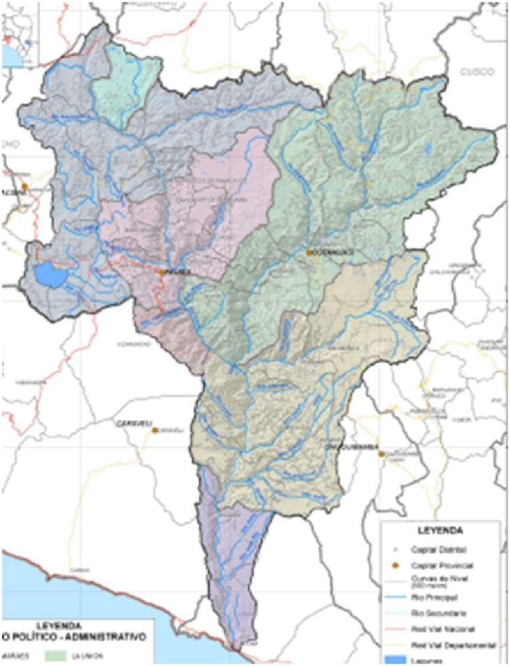
The canyon formed by the mountain range, takes the form of a wind duct (Fig. 1), which significantly increases its speed in the throat that forms it [11]. To obtain a clear assessment of the wind potential, it is necessary to carry out wind measurements in the area [12]. Data collection is done at different heights, hourly and monthly variations of wind speed are analyzed [13]. Being the chosen method to evaluate the wind conditions; the installation of anemometers, at 6, 12, and 18 m above the ground surface [14]. Speeds were recorded with an hourly periodicity, for six months; It was verified that the variation of the speed between months is insignificant, for which reason sufficient time of records was determined.

Fig. 1.

Wind pipeline formed by the mountain range, in the characteristic place, Ocoña, Arequipa, Peru (National Water Authority Source). Location of the control center (wind tower); Universal Transversal Mercator (UTM), zone 18L: 697,864 E, 8'232,644 S, 426 masl.

On the other hand, the Ocoña river concentrates a significant flow in the lower basin (450 masl) (Fig. 3), which oscillates in the approximate range of 50–500 m3/s between low water and flood; being that for ecology reasons it is not intended to build a boom, the option is to take advantage of an important flow with low hydraulic head; The control section was determined, in a place where the river is concentrated, attached to the right dam in a transversal length in the order of 30 m, the characteristic width being 200 m from the right dam to the left dam, which facilitates the bathymetry and measurement of flow velocity.

Fig. 3.

Water concentration in the basin area 16,045 km², in the characteristic place, Rio Grande, Ocoña, Arequipa, Peru (National Water Authority Source).

In order to know the area of the river section, it is necessary to perform bathymetry, which provides the location of the points of the river cross section, for which a total station is used (Fig. 4). The periodic measurement of the water level is carried out with a water level sensor (Fig. 5), another important parameter that must be recorded is the speed of the river; having periodic values, of both, and with the pre-established section of the river; we can monitor the flow, which is the data, with which we can evaluate the potential of the hydraulic resource of the characteristic place.

Fig. 4.

Bathymetry in the area where the surface runoff of the river is concentrated (adjacent to the right dike) (Own elaboration).

Fig. 5.

Record of the water level of the river, by means of a water level sensor, the measurement of the speed of the flow is carried out periodically with a current meter (Own elaboration).

3. Data and results

Wind. - By means of the three anemometers, a reading of the speed and direction of the wind was made, taking the reading every hour throughout 6 months, this information being the basis of the study of wind potential. Three organized databases are presented below, in tables, with the average (AVP). and standard deviation of the sample (D. Sta. M), for 24 h a day, according to the three anemometers placed at 6, 12 and 18 m above the surface (Fig. 2), considering the months of March to August 2022 (6 months), and their respective results (Graph 1, Graph 2, Graph 3).

Fig. 2.

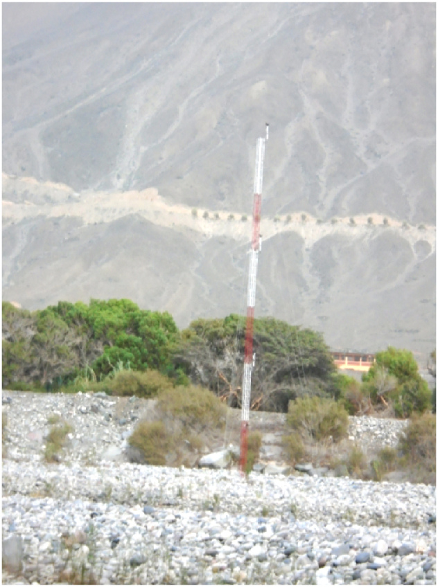
Wind tower with its three anemometers, with data logger (instrument capable of recording the intensity and direction of the wind with an hourly periodicity), booster (instrument capable of increasing the intensity of data transmission, from the data logger to the data collector), and data collector (instrument capable of storing the information from the data logger) (Own elaboration).

Graph 1.

Average wind speed and standard deviation of the records with winds greater than 6 m/s (Useable), according to the months of March to August (6 months), from the anemometer installed 6 m above the surface. (Own elaboration).

Graph 2.

Average wind speed and standard deviation of the records with winds greater than 6 m/s (Useable), according to the months of March to August (6 months), from the anemometer installed 12 m above the surface. (Own elaboration).

Graph 3.

Average wind speed and standard deviation of the records with winds greater than 6 m/s (Useable), according to the months of March to August (6 months), of the anemometer installed at 18 m above the surface (Own preparation).

With the data from Table 1, Table 2, Table 3; Graph 4 is elaborated, which represents the variation of the wind speed, according to the hours of the day, for the anemometers installed at 6, 12, and 18 m above the surface.

Table 1.

Numerical information of the anemometer installed 6 m from the surface (Own elaboration).

Hora	March	April	May	June	July	August	Aver.	Stand. Dev.
0.00	2.70	1.80	1.90	2.30	1.50	1.70	2.00	0.40
1.00	2.40	1.90	2.00	2.10	1.70	1.80	2.00	0.30
2.00	1.90	2.00	2.10	2.20	1.80	2.00	2.00	0.20
3.00	1.90	1.60	1.90	1.90	1.70	1.90	1.80	0.10
4.00	1.90	1.20	1.40	1.40	1.50	1.60	1.50	0.30
5.00	2.00	1.30	1.30	1.50	1.40	1.60	1.50	0.30
6.00	1.70	1.10	1.70	1.90	1.70	1.90	1.60	0.30
7.00	1.40	1.30	1.70	1.70	1.70	1.70	1.60	0.20
8.00	1.90	1.60	2.10	1.90	1.90	1.40	1.80	0.30
9.00	2.90	2.80	3.30	2.50	2.60	1.80	2.60	0.50
10.00	5.00	5.20	4.70	4.00	3.90	3.10	4.30	0.80
11.00	7.80	7.80	6.30	5.90	5.70	4.70	6.40	1.20
12.00	8.60	9.00	7.90	7.40	7.30	6.50	7.80	0.90
13.00	8.80	8.50	9.40	8.40	8.20	8.20	8.60	0.40
14.00	8.40	7.90	9.50	8.90	8.80	9.70	8.90	0.70
15.00	8.30	7.60	9.00	8.40	8.50	10.30	8.70	0.90
16.00	7.50	7.90	8.30	7.50	7.70	9.70	8.10	0.80
17.00	7.30	7.80	7.50	6.90	7.00	8.40	7.50	0.60
18.00	6.50	7.40	6.10	5.30	6.00	7.40	6.40	0.80
19.00	6.20	5.70	4.30	3.70	4.40	5.60	5.00	1.00
20.00	5.10	4.50	2.90	2.50	2.80	4.20	3.70	1.10
21.00	4.20	3.20	2.10	1.70	1.90	2.70	2.60	1.00
22.00	3.50	2.40	1.40	1.60	1.60	1.80	2.00	0.80
23.00	2.80	1.80	1.50	2.00	1.60	1.60	1.90	0.50

Table 2.

Numerical information of the anemometer installed 12 m from the surface (Own elaboration).

Hora	March	April	May	June	July	August	Aver.	Stand. Dev.
0.00	3.00	2.00	2.20	2.50	1.70	1.90	2.20	0.50
1.00	2.70	2.30	2.30	2.40	1.90	2.10	2.30	0.30
2.00	2.10	2.00	2.00	2.50	2.00	2.20	2.10	0.20
3.00	2.10	1.70	1.50	2.20	1.90	2.10	1.90	0.30
4.00	2.10	1.50	1.40	1.50	1.60	1.80	1.70	0.30
5.00	2.20	1.40	1.70	1.70	1.50	1.80	1.70	0.30
6.00	1.90	1.40	1.90	2.10	1.90	2.10	1.90	0.20
7.00	1.60	1.40	2.20	2.00	1.90	2.00	1.90	0.30
8.00	2.20	1.90	3.40	2.20	2.10	1.60	2.20	0.60
9.00	3.20	3.70	5.00	2.80	2.90	2.00	3.30	1.00
10.00	5.60	6.70	6.80	4.50	4.40	3.50	5.30	1.30
11.00	8.70	9.20	8.60	6.60	6.40	5.20	7.50	1.60
12.00	9.60	9.90	10.60	8.30	8.20	7.40	9.00	1.20
13.00	9.80	9.30	10.40	9.50	9.30	9.30	9.60	0.40
14.00	9.30	8.70	9.60	10.00	9.90	11.00	9.70	0.80
15.00	9.20	8.30	9.30	9.50	9.50	11.60	9.60	1.10
16.00	8.40	8.60	8.40	8.50	8.70	10.90	8.90	1.00
17.00	8.10	8.40	6.90	7.80	7.90	9.50	8.10	0.90
18.00	7.20	7.50	4.70	6.00	6.70	8.30	6.80	1.30
19.00	6.90	5.70	3.30	4.20	4.90	6.30	5.20	1.30
20.00	5.70	4.50	2.50	2.80	3.20	4.70	3.90	1.30
21.00	4.70	3.20	1.60	1.90	2.10	3.00	2.80	1.10
22.00	3.90	2.50	1.90	1.70	1.80	2.00	2.30	0.80
23.00	3.10	2.10	2.20	2.20	1.80	1.80	2.20	0.50

Table 3.

Numerical information of the anemometer installed at 18 m from the surface (Own elaboration).

Hora	March	April	May	June	July	August	Aver.	Stand. Dev.
0.00	2.70	2.40	2.40	3.00	1.90	2.20	2.40	0.40
1.00	2.50	2.50	2.60	2.70	2.10	2.30	2.40	0.20
2.00	2.60	2.60	2.60	2.80	2.20	2.50	2.50	0.20
3.00	2.60	2.10	2.40	2.40	2.20	2.30	2.30	0.20
4.00	2.10	1.60	1.90	1.80	1.90	2.00	1.90	0.20
5.00	1.90	1.70	1.70	1.90	1.70	2.00	1.80	0.10
6.00	1.80	1.50	2.10	2.30	2.00	2.30	2.00	0.30
7.00	1.70	1.60	2.20	2.10	2.10	2.10	2.00	0.20
8.00	2.00	1.70	2.50	2.40	2.30	1.80	2.10	0.30
9.00	3.70	3.20	3.60	2.80	2.90	2.00	3.00	0.60
10.00	7.00	6.30	5.50	4.50	4.40	3.50	5.20	1.30
11.00	10.20	9.50	7.50	6.90	6.70	5.40	7.70	1.80
12.00	11.10	11.20	9.80	8.70	8.60	7.70	9.50	1.40
13.00	10.90	10.80	11.90	10.10	9.90	9.90	10.60	0.80
14.00	10.20	10.20	11.90	10.80	10.70	11.90	10.90	0.80
15.00	9.90	9.70	11.20	10.50	10.50	12.80	10.70	1.10
16.00	10.00	10.00	10.50	9.40	9.70	12.20	10.30	1.00
17.00	10.30	9.90	9.30	8.60	8.80	10.50	9.50	0.80
18.00	9.30	9.20	7.40	6.60	7.30	9.10	8.10	1.20
19.00	7.60	7.00	5.30	4.50	5.30	6.70	6.10	1.20
20.00	6.10	5.50	3.70	3.00	3.50	5.10	4.50	1.30
21.00	4.60	4.00	2.60	2.10	2.30	3.30	3.20	1.00
22.00	3.60	3.10	1.90	1.90	1.90	2.10	2.40	0.70
23.00	2.70	2.40	1.90	2.40	1.90	2.00	2.20	0.30

Graph 4.

Average wind speed, according to the hours of the day, of the anemometers installed at 6, 12, and 18 m above the surface shows the speed of 6 m/s, which separates the useable wind speeds, higher than 6 m/s, of the less useable less than 6 m/s (own elaboration).

It is convenient to know the direction of the wind, for the study of the wind potential, for this a diagram called Wind rose is made (Fig. 6), shown in (Graph 5), with the WRPLOT View Freeware 8.0.2 software, and with the data of a characteristic month (August 2022), for the anemometer placed 18 m above the surface; according to the data structure required by the WRPLOT View Freeware 8.0.2 software, which is shown in (Table 4).

Fig. 6.

Location of the Wind Rose in the Control Center (wind tower); Universal Transversal Mercator (UTM), zone 18L: 697,864 E, 8'232,644 S, 426 masl, using the WRPLOT View Freeware 8.0.2 software (Own elaboration).

Graph 5.

Wind speed and direction information, using the WRPLOT View Freeware 8.0.2 software, and wind speed and direction information for a characteristic month (August 2022), from the anemometer placed 18 m above sea level. terrain, in the control tower (Own elaboration).

Table 4.

Data structure, required by the WRPLOT View Freeware 8.0.2 software (Own creation).

Day	Month	Year	Hour	Speed	Direction
1	8	2022	0	2.5	230
1	8	2022	1	2.8	206
1	8	2022	2	2.5	205
1	8	2022	3	1	192
1	8	2022	4	2.3	19
1	8	2022	5	3	11
1	8	2022	6	0.4	244
1	8	2022	7	1.6	285
1	8	2022	8	2.8	232
1	8	2022	9	2.5	223
1	8	2022	10	4	222
1	8	2022	11	4.7	241
1	8	2022	12	6.4	243
1	8	2022	13	10	244
1	8	2022	14	11.3	248
1	8	2022	15	11.8	251

WindLog Export Generated,"02/09/2022 08:37:54" Database, "UNSA-ALTO-HORA" Range,"2022-07-29","to","2022-09-02".

Mini-hydraulic. - With the data obtained from the bathymetry (Fig. 4), we proceed to carry out a periodic record of the height of the hair of water (Fig. 5), as well as the speed of the flow; From what, the periodic calculation of the control section and the surface runoff of the river is possible. During the data recording, it was observed that this flow has a great variation between flood (December, January and February) and dry season (from March to November), due to the presence or not of rain in the basin; as can be seen in Table 5.

Table 5.

River water level and surface runoff velocity, at the control station; record of water level (m), velocity (m/s).

River's level (m), and average velocity (m/s) in the registration point
	March	April	May	June	July	August
Average	2.77	1.95	1.53	1.51	1.40	1.40
Stand. Dev.	0.10	0.52	0.06	0.04	0.01	0.01
Average velocity	3.88	3.83	3.56	3.23	3.15	3.05

Des. St. Mue. - Sample standard deviation.

Water concentration in the basin area 16,045 km2, in the characteristic place, Rio Grande, Ocoña, Arequipa, Peru.

The Kaplan turbine is appropriate for small hydraulic heights between 3m and 20m, and large flows between 50m3/s to 500m3/s at the characteristic location.

4. Analysis

Wind power potential. - The useable energy depends on the wind turbine used, in this case we refer to a useable speed greater than or equal to 6 m/s, to evaluate the wind potential of the characteristic place [[15], [16], [17]]. The number of hours in which there is a speed greater than or equal to 6 m/s is considered, these being the hours that are considered useable, with their respective average wind speeds [[18], [19], [20]]. Table 6, Table 7, Table 8 show the summarized information from Table 1, Table 2, Table 3 useful for this analysis [21,22].

Table 6.

Calculated: average area (m2), average flow (m3/s), (own elaboration).

	March	April	May	June	July	August
Average Area (m2)	74	42	25	22	20	19
Average Flow (m3/s)	287	161	89	71	63	58

Table 7.

Summarized information from Table 1. (Own elaboration).

Anemometer at 6 m above surface, velocities in m/s
	March	April	May	June	July	August	Average
NHM 6 m/s	9.0	8.0	8.0	6.0	7.0	7.0	7.5 (hours)
Average velocity (m/s)	7.7	8.0	8.0	7.9	7.6	8.6	8.0 (m/s)
Stand. Dev.	0.9	0.5	1.3	0.8	1.0	1.4	1

Table 8.

Summarized information from Table 2. (Own elaboration).

Anemometer at 12 m above surface, velocities in m/s
	March	April	May	June	July	August	Average
NHM 6 m/s	9	9	8	8	8	8	8.3 (hours)
Average velocity (m/s)	8.6	8.5	8.8	8.3	8.3	9.3	8.6 (m/s)
Stand. Dev.	1	1	1.4	1.4	1.3	1.9	1.3

It can be seen that both the number of hours with useable wind speeds, and their respective wind speed averages, increase with height above the ground surface; Therefore, for a specific height, the number of hours with useable wind and its respective wind speed can be forecast. Information from the anemometer at 18 m above the ground surface is conservatively used to evaluate heights greater than or equal to 18 m.

Determination of wind potential. - To determine the potential of the wind, which can be used, the information from Table 6, Table 7, Table 8 is summarized, in Table 9, the average wind speeds, with their respective numbers of useable hours.

Table 9.

Summarized information from Table 3. (Own elaboration).

Anemometer at 18 m above surface, velocities in m/s
	Marzo	Abril	Mayo	Junio	Julio	Agosto	Promedio
NHM 6 m/s	11	10	8	8	8	8	8.8 (hours)
Average velocity (m/s)	9.3	9.4	9.9	8.9	9	10	9.4 (m/s)
Stand. Dev.	1.7	1.6	1.8	1.6	1.5	2.2	1.7

Wind Power in Kilowatts.

$$\mathrm{P}=\text{Cp}*\mathrm{\rho }*(\mathrm{\pi }/4)*\mathrm{D}2*\mathrm{V}3$$ (1)

$$\text{Cp}=0.45\mathrm{\rho }=1.29\text{Kg}/\mathrm{m}3$$

Table 10 shows the power in Kilo Watts (Kw) that can be obtained for different diameters of wind turbines; from small to the largest currently being built, with proposed turbine diameters, and recorded wind speeds at the characteristic location.

Table 10.

Summary of average speeds of wind speed, and its number of useable daily hours, according to the height of the anemometers, installed in the control tower [15,16] (Own elaboration).

Height (m)	Average velocity (m/s)	Hours of vel. 6 m/s or above
6	8	8
12	8.6	8
18	9.4	9

The power that can be used depends directly on the diameter of the blade to be used, for the wind speed conditions of the place to be considered; you can take better advantage of the wind speed, with blades of greater length (for economies of scale). But it should also be considered that the smaller blades have a lower installation cost, so they can be more easily accessible (by price); In any case, the energy demand must be evaluated, for the specific case that is considered.

For the proposal to be economically sustainable, the value of energy production must cover costs (direct, operation, and maintenance, among others), in addition to generating reasonable profits; They are evaluated, for the diameters of the proposed wind turbines; with the powers calculated in (Kw), and the number of useable wind hours per day; the energy in (kWh). With the current price of kWh: US$ 0.07/kwh established according to OSINERMING, Resolution No. 006-2022-05/CD, the production values are calculated; daily, monthly, and annual in (US$), which are presented in Table 11.

Table 11.

Power in Kw. (Own elaboration).

• Cp.- Wind utilization factor, taking into account the Betz limit, friction losses and others.
• ρ.- Air density at 20 °C and 450m.snm
• D.- Diameter of the area swept by the blades.
• V.- Wind speed.
• P.- power.

D(m)	V (m/s)	P (Kw)
6	8	8
12	8.6	42
18	9.4	123
50	9.4	947
100	9.4	3787
200	9.4	15,147

Energy production value = US$ 0.07/kwh Source. – OSINERMING, Resolution No. 006-2022-05/CD.

Small hydro power potential. - In order to evaluate the mini-hydraulic potential, offered by the Ocoña river basin, a topographic-bathymetric study was carried out, and the periodic record of the water level, and speed of surface runoff, the results of which are shown in Table 5 and Graph 6. In addition, with the statistical information from the National Water Authority Table 6, the type of turbine that is suitable for the topology described in Graph 7 is selected, as well as in Graph 8, it is exemplified that, given the characteristic shape of the basin, it is not difficult to achieve a small hydraulic height, with a small path, between intake and delivery to the Kaplan-type mini turbine (see Graph 9).

Graph 6.

Cross section of the Ocoña river, Arequipa, Peru, UTM 18L, 697787 E, 8232650 S, 425 masl. Width of the river from dam to dam: 182.48 m Vertical Scale = Horizontal Scale x10 (Own elaboration).

Graph 7.

Persistence curve of the Ocoña river, Arequipa, Peru. (Source National water Authority).

Graph 8.

Choice of the type of turbine. (Own elaboration).

Graph 9.

Given the topology, it is not difficult to achieve a small hydraulic head; For example, in the characteristic place in the Ocoña river: Hydraulic Load H = 20 m. (Own elaboration).

Mini-hydraulic power in Kilowatts

$$\mathrm{P}=\mathrm{\eta }*\mathrm{\gamma }*\mathrm{Q}*\mathrm{H}$$ (2)

$$\text{Efficiency}\mathrm{\eta }=0.8\mathrm{\gamma }=1,000\text{KgF}/\mathrm{m}3$$

$$\text{We}\text{consider}\mathrm{H}=20\mathrm{m}$$

Similar to Table 12, it has been considered, to exemplify, a small hydraulic height of 20 m, with different flows, which it is possible to capture, considering the exposed topology, the number of hours a day is complete; 24 h, a typical overall efficiency of 80 % has been considered, and the specific weight of water 1,000 KgF/m3.

Table 12.

Value of energy production in US$. (Own elaboration).

D(m)	P (Kw)	Hours/Day	E (Kwh)	Daily production value (U.S.$)	Monthly production value (U.S.$)	Anual production value (U.S.$)
6	8	8	67	5	141	1,718
12	42	8	334	23	702	8,536
18	123	9	1,104	77	2,319	28,213
50	947	9	8,520	596	17,893	217,695
100	3,787	9	34,081	2,386	71,571	870,781
200	15,147	9	136,326	9,543	286,284	3,483.125

With this information, considering that the dry season is ¾ parts of the year where there are flows in the order of 50 cubic meters per second, with a persistence greater than or equal to 90 %, and that the flood season is ¼ part of the year, a period in which persistence is also high. Considering the current price of kWh: US$ 0.07/kwh established according to OSINERMING, Resolution No. 006-2022-05/CD, the production values are calculated in Table 13; daily, monthly, and yearly in (US$).

Table 13.

Value of production in US $. (Own elaboration).

Q (m³/s)	P (Kw)	Hours/Day	E (Kwh)	Daily production value (U.S.$)	Monthly production value (U.S.$)	Anual production value (U.S.$)
5	785	24	18,835	1,318	39,554	481,239
10	1,570	24	37,670	2,637	79,108	962,479
20	3,139	24	75,341	5,274	158,216	1,924,957
50	7,848	24	188,352	13,185	395,539	4,812,394
100	15,696	24	376,704	26,369	791,078	9,624,787
200	31,392	24	753,408	52,739	1,582,157	19,249,574
450	70,632	24	1,695,168	118,662	3,559,853	43,311,542

According to the regulations of each country, the ecological flow should be considered.

Economic technical potential of the hybrid system. – It is considered that to satisfy the domestic demand (population) the mini-hydraulic system is appropriate, which has the advantage of a daily persistence of 100 %, thus taking a small hydraulic flow (10 % of the hydraulic flow of the river in low water), it is It can have an annual production value (US$ 481,239) that guarantees the economic sustainability of the mini-hydraulic system. On the other hand, to satisfy industrial demand, the wind system is appropriate, which only has a daily persistence of 33.4 %, thus a 200 m diameter turbine can have an annual production value (US$ 3,483,125). that guarantees the economic sustainability of the wind system; For these reasons, the economic technical potential of the hybrid system is appropriate to satisfy the domestic demand and the industrial demand for electrical energy.

5. Conclusions

From six months of wind observations, it was noted that there is no significant variation between the months, more so between the hours. The speed is frankly useable, in the order of 9 m/s, with a persistence in the order of 8 h a day (Table 9). According to the analysis of the wind potential of the area. Wind speed increases with height. (Graph 4).

Regarding the mini-hydraulic use, there is no major limitation, since the essential demands can be easily covered with the flow available 24 h a day, and obtaining the hydraulic height is not difficult either, given the topology of the mountain range (Graph 8), (Table 12). The level of the river, and consequently its flow, has a clear variation with the change from flood to low water, and vice versa; that must be taken into account. (Table 5).

The use of wind energy is possible with current technology, it also has the flexibility to adapt to investments of different sizes with their respective returns.

The fact that the useable winds are in approximately one third of the day, can be overcome by considering pumping the water from the river, to have a gravity storage, for agriculture, mining, green hydrogen generation, among others.

The use of mini-hydraulic energy has the advantage of being continuous, being able to satisfy the essential demands with ease.

The combined use, allows to satisfy the essential demand, with the mini-hydraulic energy, and one with ease and variability of investment; using wind energy, for industrial uses, such as agriculture, mining, green hydrogen among others.

6. Recommendations

It is recommended to make the precisions to adapt to the demand that is considered. Deepen the studies of the appropriate equipment for the use of wind, mini-hydraulic, and combined energy; considering the accessibility of the investment required, and the profitability of the economy of scale, in contrast.

Recognition

To the National University of San Agustín de Arequipa, for financing this applied research, Financing Contract No. IBA-IB-29-2020-UNSA, Call 2019-1.

To the Ph.D. Marcelo Mariz Veiga for guiding our research and facilitating the publication of this paper.

Data availability

The data is available upon request.

Ethics declarations

Review and/or approval by an ethics committee was not needed for this study.

CRediT authorship contribution statement

José Luis Salas Gonzales: Investigation. Alembert Delfin Hilario Huaccha: Investigation. Kent Rodrigo Mamani Hilasaca: Investigation. Walid Andy Kana Hancco: Investigation. David Tunti Alanocca: Investigation. Duval Bremell Cruz Mamani: Investigation. Jordán Sebastián Llave Halanoca: Investigation. Willy Roberto López Tejada: Investigation.

Declaration of competing interest

The authors declare the following financial interests/personal relationships which may be considered as potential competing interests:MSC ING JOSE LUIS SALAS GONZALES reports financial support was provided by UNIVERSIDAD NACIONAL DE SAN AGUSTIN DE AREQUIPA.

References

- 1.Nurulkamal Masseran. Evaluating wind power density models and their statistical properties. Energy. 2015;84:533–541. doi: 10.1016/j.energy.2015.03.018. [DOI] [Google Scholar]
- 2.Justus C.∼G., Mikhail A. Height variation of wind speed and wind distributions statistics. \grl. May 1976;3(5):261–264. doi: 10.1029/GL003i005p00261. [DOI] [Google Scholar]
- 3.Chou Karen C., Corotis Ross B. Simulation of hourly wind speed and array wind power. Sol Energy. 1981;26(3):199–212. doi: 10.1016/0038-092X(81)90204-8. [DOI] [Google Scholar]
- 4.Gugliani G.K., Sarkar A., Ley C. y, Matsagar V. Identification of optima wind aerogeneradores para varios climas eólicos usando un nuevo índice de rendimiento de la turbina basado en meses. Energía Removable. 2021;171:902–914. [Google Scholar]
- 5.Shoaib M., Siddiqui I., Rehman S., Khan S., Alhems L.M. Assessment of wind energy potential using wind energy conversion system. J. Clean. Prod. 2019;216:346–360. doi: 10.1016/j.jclepro.2019.01.128. [DOI] [Google Scholar]
- 6.Khalid Saeed M., Salam A., Rehman A.U., Abid Saeed M. Comparison of six different methods of Weibull distribution for wind power assessment: a case study for a site in the Northern region of Pakistan. Sustain. Energy Technol. Assessments. 2019;36 doi: 10.1016/j.seta.2019.100541. [DOI] [Google Scholar]
- 7.Wen Jiang, Yan Zheng, Feng Donham. A review on reliability assessment for Wind power. Renew Sustain Energy Rev. 2009;13(9):2485–2494. doi: 10.1016/j.rser.2009.06.006. [DOI] [Google Scholar]
- 8.Saleh H., Abou El-Azm Aly A., Abdel-Hady S. Assessment of different methods used to estimate Weibull distribution parameters for wind speed in Zafarana wind farm, Suez Gulf, Egypt. Energy. 2012;44(1):710–719. doi: 10.1016/j.energy.2012.05.021. [DOI] [Google Scholar]
- 9.Weisser Daniel. A wind energy analysis of Grenada: an estimation using the ‘Weibull’ density function. Renew Energy. 2003;28(11):1803–1812. doi: 10.1016/S0960-1481(03)00016-8. [DOI] [Google Scholar]
- 10.Dragica J., Škerlavaj A., Andrej L. Improvement of efficiency prediction for a kaplan turbine with advanced turbulence models. Turboinštitut, Journal of Mechanical Engineering, Slovenia. 2014 doi: 10.5545/sv-jme.2013.1222. [DOI] [Google Scholar]
- 11.Corotis Ross B., Sigl Arden B., Klein Joel. Probability models of wind velocity magnitude and persistence. Sol Energy. 1978;20(6):483–493. doi: 10.1016/0038-092X(78)90065-8. [DOI] [Google Scholar]
- 12.Costa Rocha P.A., de Sousa R.C., de Andrade C.F., da Silva M.E.V. Comparison of seven numerical methods for determining Weibull parameters for wind energy generation in the northeast region of Brazil. Appl. Energy. 2012;89(1):395–400. doi: 10.1016/j.apenergy.2011.08.003. [DOI] [Google Scholar]
- 13.Fazelpour F., Soltani N., Soltani S., Rosen M.A. Assessment of wind energy potential and economics in the north-western Iranian cities of Tabriz and Ardabil. Renew. Sustain. Energy Rev. 2015;45:87–99. doi: 10.1016/j.rser.2015.01.045. [DOI] [Google Scholar]
- 14.Wais P. A review of Weibull functions in wind sector. Renew. Sustain. Energy Rev. Apr. 2017;70:1099–1107. doi: 10.1016/j.rser.2016.12.014. [DOI] [Google Scholar]
- 15.Bardsley W.E. Note on the use of the inverse Gaussian distribution for wind energy applications. J Appl Meteorol. 1980;19(9):1126–1130. doi: 10.1175/1520-0450(1980)019%3C1126:NOTUOT%3E2.0.CO;2. [DOI] [Google Scholar]
- 16.Péter Kiss, Jánosi Imre M. Comprehensive empirical analysis of ERA-40 surface wind speed distribution over Europe. Energy Convers Manage. 2008;49(8):2142–2151. doi: 10.1016/j.enconman.2008.02.003. [DOI] [Google Scholar]
- 17.Kaplan Y.A. Performance assessment of power density method for determining the weibull distribution coefficients at three different locations. Flow Meas. Instrum. Oct. 2018;63:8–13. doi: 10.1016/j.flowmeasinst.2018.07.004. [DOI] [Google Scholar]
- 18.Abdul Baseer Mohammed, Meyer J.P., Rehman Md S., Mahbub Alamad. Wind power characteristics of seven data collection sites in Jubail, Saudi Arabia using Weibull parameters. Renew Energy. 2017;102:35–49. doi: 10.1016/j.renene.2016.10.040. [DOI] [Google Scholar]
- 19.Celik A.N. Weibull representative compressed wind speed data for energy and performance calculations of wind energy systems. Energy Convers Manage. 2003;44(19):3057–3072. doi: 10.1016/S0196-8904(03)00075-X. [DOI] [Google Scholar]
- 20.Soon-Duck Kwon. Uncertainty analysis of wind energy potential assessment. Appl Energy. 2010;87(3):856–865. doi: 10.1016/j.apenergy.2009.08.038. [DOI] [Google Scholar]
- 21.Shahnawaz Farhan Khahro, Amir Mahmood Soomro, Kavita Tabbassum. Assessment of wind power potential at hawksbay, Karachi Sindh, Pakistan. Indonesian J Electr Eng Comput Sci. 2013;11(7):3479–3490. doi: 10.11591/telkomnika.v11i7.2621. [DOI] [Google Scholar]
- 22.Irfan Ullah, Chipperfield Andrew J. An evaluation of wind energy potential at Kati Bandar, Pakistan. Renew Sustain Energy Rev. 2010;14(2):856–861. doi: 10.1016/j.rser.2009.10.014. [DOI] [Google Scholar]
Associated Data
This section collects any data citations, data availability statements, or supplementary materials included in this article.
Data Availability Statement