Abstract
The problem of image restoration in cryo-EM entails correcting for the effects of the Contrast Transfer Function (CTF) and noise. Popular methods for image restoration include ‘phase flipping’, which corrects only for the Fourier phases but not amplitudes, and Wiener filtering, which requires the spectral signal to noise ratio. We propose a new image restoration method which we call ‘Covariance Wiener Filtering (CWF). In CWF, the covariance matrix of the projection images is used within the classical Wiener filtering framework for solving the image restoration deconvolution problem. Our estimation procedure for the covariance matrix is new and successfully corrects for the CTF. We demonstrate the efficacy of CWF by applying it to restore both simulated and experimental cryo-EM images. Results with experimental datasets demonstrate that CWF provides a good way to evaluate the particle images and to see what the dataset contains even without 2D classification and averaging.
Keywords: CTF correction, Steerable PCA, Wiener filtering
1. Introduction
Single particle reconstruction (SPR) using cryo-electron microscopy (cryo-EM) is a rapidly advancing technique for determining the structure of biological macromolecules at near-atomic resolution directly in their native state, without any need for crystallization (Bai et al., 2015; Milne et al., 2013; Nogales, 2016; Sigworth; Kühlbrandt, 2014). In SPR, 3D reconstructions are estimated by combining multiple noisy 2 D tomographic projections of macromolecules in different unknown orientations.
The acquired data consists of multiple micrographs from which particle images are extracted in the first step of the computational pipeline. Next, the images are grouped together by similarity in the 2D classification and averaging step (Zhao and Singer, 2014; Park and Chirikjian, 2014). Class averages can be used to inspect the underlying particles, and to estimate viewing angles and form a low resolution ab initio 3D model. Subsequently, this 3D model is refined to high resolution, and 3D classification might be performed as well.
In this paper we propose an image restoration method that provides a way for visualizing the particle images without performing any 2D classification. While noise reduction is achieved in 2D classification by averaging together different particle images, our method operates on each image separately, and performs Contrast Transfer Function (CTF) correction and denoising in a single step.
Existing image restoration techniques (for denoising and CTF correction) can be broadly categorized into two kinds of approaches (Penczek, 2010). The first is an approach known as ‘phase flipping’, which involves flipping the sign of the Fourier coefficients at frequencies for which the CTF is negative. Consequently, phase flipping restores the correct phases of the Fourier coefficients, but ignores the effect of the CTF on the amplitudes. Phase flipping preserves the noise statistics and is easy to implement, leading to its widespread usage in several cryo-EM software packages. However, it is suboptimal because it does not restore the correct Fourier amplitudes of the images. The second commonly used approach is Wiener filter based restoration, to which we refer here as traditional Wiener filtering (TWF). Wiener filtering takes into account both the phases and amplitudes of the Fourier coefficients, unlike phase flipping. However, calculation of the Wiener filter coefficients requires prior estimation of the spectral signal to noise ratio (SSNR) of the signal, which by itself is a challenging problem. It is therefore customary to either treat the SSNR as a precomputed constant as in the software package SPIDER (Frank et al., 1996), or to apply Wiener filtering only at later stages of the 3D reconstruction pipeline when the noise level is sufficiently low, such as in EMAN2 (Tang et al., 2007). It is also possible to use a combination of the two approaches, by first phase flipping the 2D images, and later correct only for the amplitudes in the 3D reconstruction step, as in IMAGIC (van Heel et al., 1996; van Heel et al., 2000). Despite its simplicity, there are several drawbacks to TWF. First, it cannot restore information at the zero crossings of the CTF. Second, it requires estimation of the SSNR. Third, it is restrictive to the Fourier basis which is a fixed basis not adaptive to the image dataset.
We refer to our proposed method as Covariance Wiener Filtering (CWF). CWF consists of first estimating the CTF-corrected covariance matrix of the underlying clean 2D projection images, followed by application of the Wiener filter to denoise the images. Unlike phase flipping, CWF takes into account both the phases and magnitudes of the images. Moreover, unlike TWF that always operates in the data-independent Fourier domain, CWF is performed in the data-dependent basis of principal components (i.e., eigenimages). Crucially, CWF can be applied at preliminary stages of data processing on raw 2D particle images. The resulting denoised images can be used for an early inspection of the dataset, to identify the associated symmetry, and to eliminate ‘bad’ particle images prior to 2D classification and 3D reconstruction. Additionally, the estimation of the 2D covariance matrix is itself of interest, for example, in Kam’s approach for 3D reconstruction (Kam, 1980; Bhamre et al., 2015).
The paper is organized as follows: Sections 2.1 and 2.2 detail the estimation of the covariance matrix for two different noise models, first for the simpler model of white noise, and second for the more realistic model of colored noise. In Section 2.3 we discuss the steerability property of the covariance matrix (Zhao et al., 2016). The associated deconvolution problem is solved to obtain denoised images using the estimated covariance matrix in Section 2.4. Finally in Section 3, we demonstrate CWF in a number of numerical experiments, with both simulated and experimental datasets. We obtain encouraging results for experimental datasets, in particular, those acquired with the modern direct electron detectors. Image features are clearly observed after CWF denoising. For reproducibility, the MATLAB code for CWF and its dependencies are available in the open source cryo-EM toolbox ASPIRE at www.spr.math.princeton.edu. The script cwf_script.m, calls the main function cwf.m
2. Methods
The first step of CWF is estimation of the covariance matrix of the underlying clean images, to which we refer as the population covariance. The second step of CWF is solving a deconvolution problem to recover the underlying clean images using the estimated covariance. In the rest of this section, we describe these steps in detail.
2.1. The model
The image formation model in cryo-EM under the linear, weak phase approximation (Frank, 1996) is given by
| (1) |
where is the number of images, * denotes the convolution operation, is the noisy, CTF filtered ith image in real space, is the underlying clean projection image in real space, is the point spread function of the microscope that convolves with the clean image in real space, and is additive Gaussian noise that corrupts the image, for each . Taking the Fourier transform of Eq. (1) gives
| (2) |
where and are now in Fourier space. is a diagonal operator, whose diagonal consists of the Fourier transform of the point spread function, and is also commonly known as the CTF. The CTF modulates the phases and the amplitudes of the Fourier coefficients of the image, and contains numerous zero crossings that correspond to frequencies at which no information is obtained. Any image restoration technique that aims to completely correct for the CTF must therefore correctly restore both the phases and the amplitudes. The zero crossings make CTF correction challenging since it cannot be trivially inverted. In experiments, different groups of images are acquired at different defocus values, in the hope that information that is lost from one group could be recovered from another group that has different zero crossings. In the experimental datasets used in this paper, the number of images per defocus group typically ranges from 50 to 1000.
In our statistical model, the Fourier transformed clean images (viewed, for mathematical convenience, as vectors in , where is the number of pixels) are assumed to be independent, identically distributed (i.i.d.) samples from a distribution with mean and covariance . Since the clean images are two-dimensional projections of the three-dimensional molecule in different orientations, the distribution of in our model is determined by the three-dimensional structure, the distribution of orientations, the varying contrast due to changes in ice thickness, and structural variability, all of course unknown at this stage. The covariance matrix therefore represents the overall image variability due to these determinants. While these model assumptions do not necessarily hold in reality (Sorzano et al., 2007; Sorzano et al., 2015), they simplify the analysis and, as will be shown later lead to excellent denoising. Quoting George Box, “All models are wrong but some are useful” (Box, 1976).
Our denoising scheme requires and . Since these quantities are not readily given, we estimate them from the noisy images themselves as follows. For simplicity, we first assume that the noise in our model is additive white Gaussian noise such that in Eq. (2) are i.i.d. The white noise assumption is later replaced by that of the more realistic colored noise. First, notice from Eq. 2 it follows that
| (3) |
So,
| (4) |
Eq. (4) relates the second order statistics of the noisy images with the population covariance of the clean images, based on which we can estimate .
Next, we construct estimators for the mean and population covariance using Eqs. (3) and (4). The mean of the dataset can be estimated as the solution to a least squares problem
| (5) |
where is a regularization parameter. The solution to 5 is explicitly
| (6) |
The population covariance can be estimated as
| (7) |
where and is the Frobenius matrix norm. The estimators and can be shown to be consistent in the large sample limit , similar to the result in Appendix B of Katsevich et al. (2015).
To ensure that the estimated covariance is positive semidefinite (PSD), we project it onto the space of PSD matrices by computing its spectral decomposition and retaining only the non negative eigenvalues (and their corresponding eigenvectors). To solve Eq. (7), we differentiate the objective function with respect to and set the derivative to zero. This yields
| (8) |
Eq. (8) defines a system of linear equations for the elements of the matrix . However, direct inversion of this linear system is slow and computationally impractical for large image sizes. Notice that Eq. (8) can be written as
| (9) |
where is the linear operator acting on defined by the left hand side of Eq. (8), and is the right hand side. Since applying only involves matrix multiplications, it can be computed fast, and the conjugate gradient method is employed to efficiently compute instead of direct inversion, similar to how it is used in Andén et al. (2015).
Notice that is a PSD matrix whenever is PSD (as a sum of PSD matrices), while may not necessarily be PSD due to finite sample fluctuations (i.e., is finite). It is therefore natural to project onto the cone of PSD matrices. This amounts to computing the spectral decomposition of and setting all negative eigenvalues to 0, which is an instance of eigenvalue thresholding.
We now describe an alternate eigenvalue thresholding procedure, better suited to cases in which the number of images is not exceedingly large. To that end, we first analyze the matrix when for all , i.e., the input images are white noise images containing no signal. Let
| (10) |
Then, and . Let , i.e. is PSD and . Then multiplying both sides of Eq. (9) with we get
| (11) |
can be viewed as a sample covariance matrix of vectors in whose population covariance is the identity matrix. When is fixed and goes to infinity, all eigenvalues of converge to 1. In practice, however, and are often comparable. In the limit and with , the limiting spectral density of the eigenvalues converges to the Marčenko Pastur (MP) distribution (Marčenko and Pastur, 1967), given by
| (12) |
for . It is therefore expected that would have eigenvalues (considerably) larger than 1, even in the pure white noise case. These large eigenvalues should not be mistakingly attributed to signal. In the case of images containing signal (plus noise), eigenvalues corresponding to the signal can only be detected if they reside outside of the support of the MP distribution. We use the method of Kritchman and Nadler (2008) to determine the number of eigenvalues corresponding to the signal. We then apply the operator norm eigenvalue shrinkage procedure (see Donoho et al.) to those eigenvalues, while setting all other eigenvalues to 0. We then use the conjugate gradient method1 to solve Eq. (11) for , with the right hand side replaced with its shrinkage version. We observed in numerical simulations (see Fig. 3) that this procedure typically out-performs other shrinkage methods in terms of the accuracy of the estimated covariance matrix.
Fig. 3.
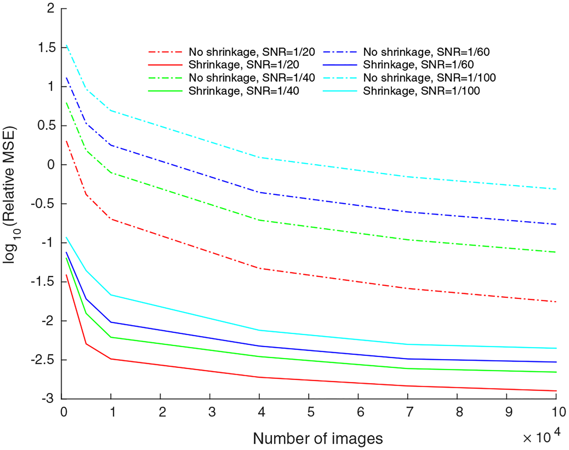
Relative MSE of the estimated covariance versus the number of images: The relative MSE of the estimated covariance , with and without using eigenvalue shrinkage, as a function of number of images, for synthetic data generated using EMDB-6454.
2.2. Covariance estimation with colored noise
So far, we assumed additive white Gaussian noise in the image formation process. In reality, the noise in experimental images is colored. That is, in the image formation model in Eq. (2), is additive colored Gaussian noise. We preprocess the images in order to “whiten” the noise. The noise power spectrum can be estimated, for example, using the pixels in the corners of the noisy projection images. To do this, we first estimate using correlograms the 2D autocorrelation of the corner pixels of the images which contain mostly noise and no signal. These corner pixels are used to estimate the 1 D autocorrelation, which is then extended to populate the 2D isotropic autocorrelation. We then calculate the Fourier transform of the 2D autocorrelation, which is the 2D power spectrum of noise. The noisy projection images in Fourier space are multiplied element-wise by the inverse of the estimated power spectral density, also called the whitening filter, so that the noise in the resulting images is approximately white. Let be the “whitening” filter, such that
| (13) |
and .
Eq. (13) is reminiscent of Eq. (2). It is tempting to define a new “effective” CTF as and estimate following the same procedure as in the case of white noise. However, the linear system akin to Eq. (8) for this case is ill-conditioned due to the product of with the CTF, and it takes a large number of iterations for conjugate gradient to converge to the desired solution. Instead, we seek an approach in which the linear system to solve is well conditioned as that in the case of white noise. Since the CTF’s and the whitening filter are diagonal operators in the Fourier basis, they commute, and Eq. (13) becomes
| (14) |
We therefore absorb into , and estimate the matrix (the population covariance of ) using the same procedure as before. The population covariance is then estimated as
| (15) |
2.3. Fourier-Bessel steerable PCA
The population covariance matrix must be invariant under inplane rotation of the projection images, therefore it is block diagonal in any steerable basis in which the basis elements are outer products of radial functions and angular Fourier modes. Following (Zhao et al., 2016), we choose to represent the images in a Fourier-Bessel basis and it suffices to estimate each diagonal block , corresponding to the angular frequency , separately. The Fourier-Bessel basis (Zhao et al., 2016) consists of basis functions (that satisfy the sampling criterion) for each angular frequency , where decreases with increasing . The matrix is thus of size .
An important property of the CTF’s and the whitening filter is that they are radially isotropic.2 Therefore, the CTF’s and the whitening filter are also block diagonal in the Fourier Bessel basis. Eq. (8) (and its analog in the case of colored noise) is hence solved separately for each to estimate .
2.4. Wiener filtering
The estimated covariance is further used to solve the associated deconvolution problem in Eq. (2) using Wiener filtering. The result is a denoised, CTF corrected image for each noisy, CTF affected measurement for . We estimate in the white noise model using the Wiener filtering procedure as
| (16) |
where is the linear Wiener filter (MacKay, 2004). In the case of colored noise,
| (17) |
with . Since the estimated covariance is block-diagonal in the Fourier Bessel basis, the Wiener filtering procedure is applied to the Fourier Bessel coefficients of the noisy images for each angular frequency separately. The denoised Fourier Bessel expansion coefficients are used to reconstruct denoised images in Fourier space that are inverse Fourier transformed to acquire images in real space on a Cartesian grid.
2.5. Computational complexity
In practice, instead of each image being affected by a distinct CTF, all images within a given defocus group have the same CTF. So, given defocus groups with images in group , one can equivalently minimize the objective function in Eq. (7) (here denotes the CTF of the ’th defocus group, and index images in that group). As a result, the sums in Eq. (8) range from 1 to instead of from 1 to , thereby reducing the computational cost of some operations. For images of size , estimating the mean using Eq. (6) takes (since is diagonal in the Fourier basis for each ). Computing the Fourier Bessel expansion coefficients takes , as detailed in Zhao et al. (2016). When solving the linear system in Eq. (8) to estimate each separately, the matrices in Eq. (8) are of size . It is shown in Zhao et al. (2016) that , and . While solving Eq. (9) using conjugate gradient for a given angular frequency, computing the action of the linear operation on takes per iteration, while computing takes . Thus, each iteration of conjugate gradient takes , that is, and there is also a one time computation of . Wiener filtering the Fourier Bessel coefficients of an image for a given angular frequency takes . So the overall complexity for Wiener filtering the coefficients of all images is . In summary, the overall complexity for CWF is , where is the number of conjugate gradient iterations.
3. Results
In this section, we apply our algorithm to synthetic and experimental datasets to obtain denoised images. All algorithms are implemented in the UNIX environment, on a machine with 60 cores, running at 2.3 GHz, with total RAM of 1.5 TB. We perform numerical experiments with (i) a synthetic dataset with additive white and colored Gaussian noise and (ii) four experimental datasets, two of which were acquired with older detectors, and the other two with state-of-the-art direct electron detectors. For all the experimental datasets, the corresponding estimated CTF parameters were provided with the dataset. For all simulations, we use centered projection images. The algorithm does not require centered images. However, having non-centered images would result in an additional ‘blurring’ effect in the denoised images.
3.1. Simulated noisy dataset with white noise
For the first experiment with simulated data, we construct a synthetic dataset by modeling the image formation process in cryo-EM. The synthetic dataset is prepared from the 3D structure of the Plasmodium falciparum 80S ribosome bound to E-tRNA, available on the Electron Microscopy Data Bank (EMDB) as EMDB-6454. We first generate clean 2D projection images starting from a 3D volume, at directions sampled uniformly over the sphere, and then corrupt the generated clean projection images with different CTF’s and additive white Gaussian noise. The projection images are divided into 10 defocus groups, with the defocus value ranging from to . The B-factor of the decay envelope was chosen as 10 Å2, the amplitude contrast as 7%, the voltage as 300 kV, and the spherical aberration as 2 mm. To ensure that the denoising quality of CWF is robust to the mean estimation of the dataset, the regularization parameter in the least squares mean estimation in Eq. (6) was fixed at 1 for all the experiments described here.
Fig. 1 shows the results of denoising raw, CTF-affected noisy images with CWF and TWF at various levels of the SNR. We have used the EMAN2 (Tang et al., 2007) implementation of TWF (note that we perform phase flipping followed by TWF only on the raw images in EMAN2, and not on averages). The SNR used here is defined relative to the CTF affected images that constitute the clean signal, and is calculated as an average value for the entire dataset. Using 20 cores, calculating the Fourier Bessel coefficients took 79 s while covariance estimation and Wiener filtering together took 6 s in the experiment with SNR=1/60.
Fig. 1.
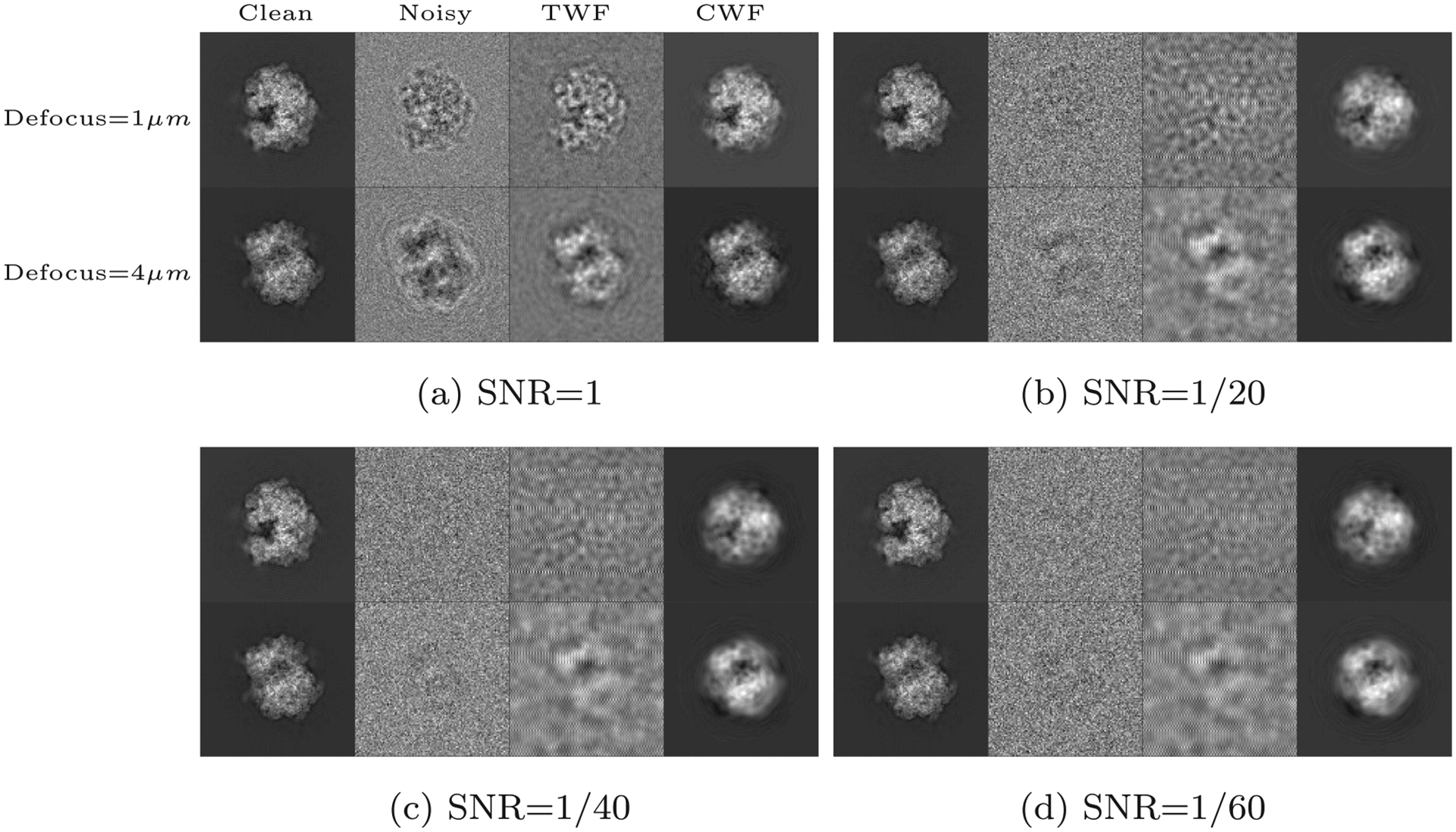
Synthetic white noise: A comparison of the denoising results of traditional Wiener filtering (TWF) and CWF for the synthetic dataset prepared from EMDB-6454, the P. falciparum 80S ribosome bound to E-tRNA. The dataset consists of 10,000 images of size 105 × 105, which are divided into 10 defocus groups, with the defocus value ranging from to . The two rows in each subfigure correspond to two clean images belonging to different defocus groups; the first one belongs to the group with the smallest defocus value of , while the second image belongs to the group with the largest defocus value of .
It is seen that TWF works very well at high SNR (⩾ 1), but deteriorates at lower SNR’s as expected. Note that the denoising results of TWF depend strongly on the defocus value. The location of the zeros in the CTF is such that images corresponding to high defocus values preserve low frequency information, while images corresponding to low defocus values retain more high frequency information. With CWF, there is no such strong dependence on the defocus value, since the covariance matrix is estimated using information from all defocus groups.
Fig. 2a shows the relative MSE of denoised images as a function of the SNR of the dataset. The MSE (norm of the difference between the denoised image and the original, clean image) shown here corresponds to the same range of SNR’s (from 1/60 to 1) as in Fig. 1. Fig. 2b shows the relative MSE of the denoised images as a function of the number of images used to estimate the covariance in the experiment. The covariance estimation improves as the number of images in the dataset increases, and so the denoising is also expected to improve, as seen from Fig. 2b.
Fig. 2.
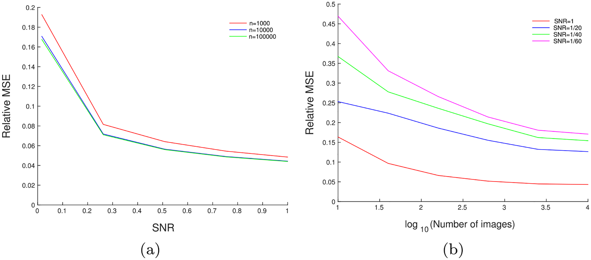
(a) Relative MSE versus the SNR, for a fixed number of images: The relative MSE of the denoised images as a function of the SNR, for synthetic data generated using EMDB-6454. The MSE reported here is averaged over all images. denotes the number of images used in the experiment. (b) Relative MSE versus the number of images, for a fixed SNR: The relative MSE of the denoised images as a function of the number of images, for synthetic data generated using EMDB-6454. The MSE reported here is averaged over all images.
The importance of the eigenvalue shrinkage procedure is elucidated in Fig. 3. Here, we compare the error in the estimated covariance with and without eigenvalue shrinkage, for varying number of images used in the experiment. The relative MSE of the estimated covariance is defined as
| (18) |
3.2. Simulated noisy dataset with colored noise
The noise that corrupts images in cryo-EM is not perfectly white, but often colored. To simulate this, we perform experiments with synthetic data generated from EMDB-6454 as described in 3.1, this time adding colored Gaussian noise with the noise response is the radial frequency) to each clean, CTF-affected projection image. Fig. 4 shows the denoised images for this case.
Fig. 4.
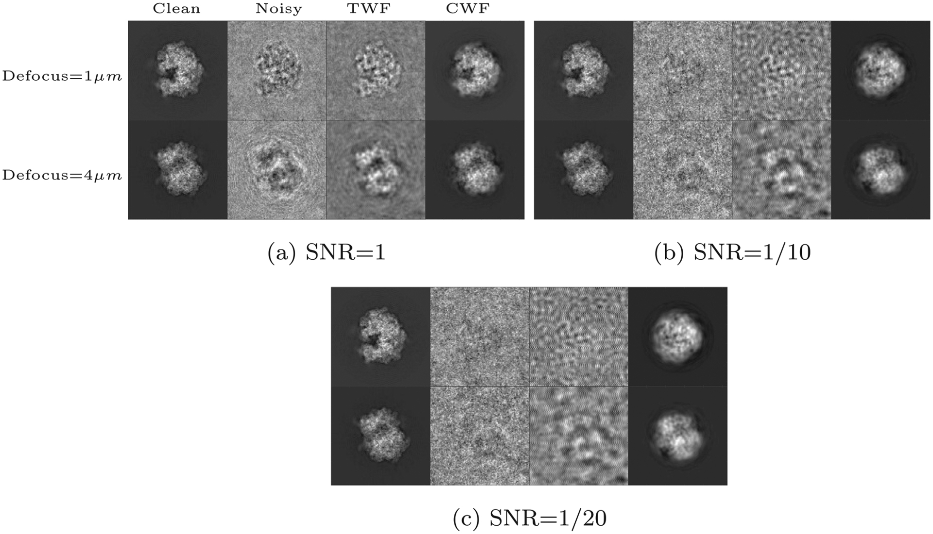
Synthetic colored noise: Denoising results of CWF for the synthetic dataset with additive colored Gaussian noise, prepared from EMDB-6454, the P. falciparum 80S ribosome bound to E-tRNA, as detailed in the caption of Fig. 1.
3.3. Experimental dataset - TRPV1
We apply CWF to an experimental dataset of the TRPV1 ion channel, taken using a K2 direct electron detector. It is available on the public database Electron Microscope Pilot Image Archive (EMPIAR) as EMPIAR-10005, and the 3D reconstruction is available on EMDB as EMDB-5778, courtesy of Liao et al. (Liao et al., 2013). The dataset consists of 35,645 motion corrected, picked particle images of size 256 × 256 pixels with a pixel size of 1.2156 Å. Using 20 cores, calculating the Fourier Bessel coefficients took 312 s while covariance estimation and Wiener filtering together took 574 s. The result is shown in Fig. 5. CWF retains 384 eigenvalues of .
Fig. 5.
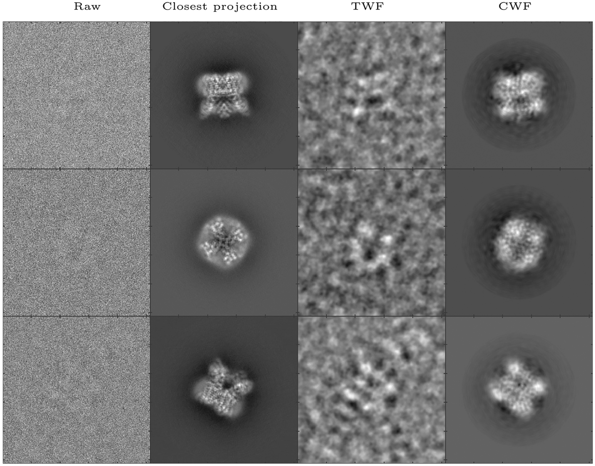
Denoising an experimental dataset of TRPV1 (Liao et al., 2013): Here we show, for three images in the dataset, the raw image, the closest true projection image generated from the 3D reconstruction of the molecule (EMDB 5778), the denoised image obtained using TWF, and the denoised image obtained using CWF. In this experiment, 35,645 images of size 256 × 256 belonging to 935 defocus groups were used. The amplitude contrast is 10%, the spherical aberration is 2 mm, and the voltage is 300 kV.
3.4. Experimental dataset - 80S ribosome
We apply CWF to an experimental dataset of the Plasmodium falciparum 80S ribosome bound to the anti-protozoan drug emetine, taken using a FEI FALCON II 4k × 4k direct electron detector. The raw micrographs and picked particles are available on the public database EMPIAR as EMPIAR-10028, and the 3D reconstruction is available on EMDB as EMDB-2660, courtesy of Wong et al. (2014). The dataset we used was provided by Dr. Sjors Scheres, and consists of 105,247 motion corrected, picked particle images of size 360 × 360 with a pixel size of 1.34 Å. Using 20 cores, calculating the Fourier Bessel coefficients took 731 s while covariance estimation and Wiener filtering together took 385 s. The result is shown in Fig. 6. CWF retains 962 eigenvalues of .
Fig. 6.
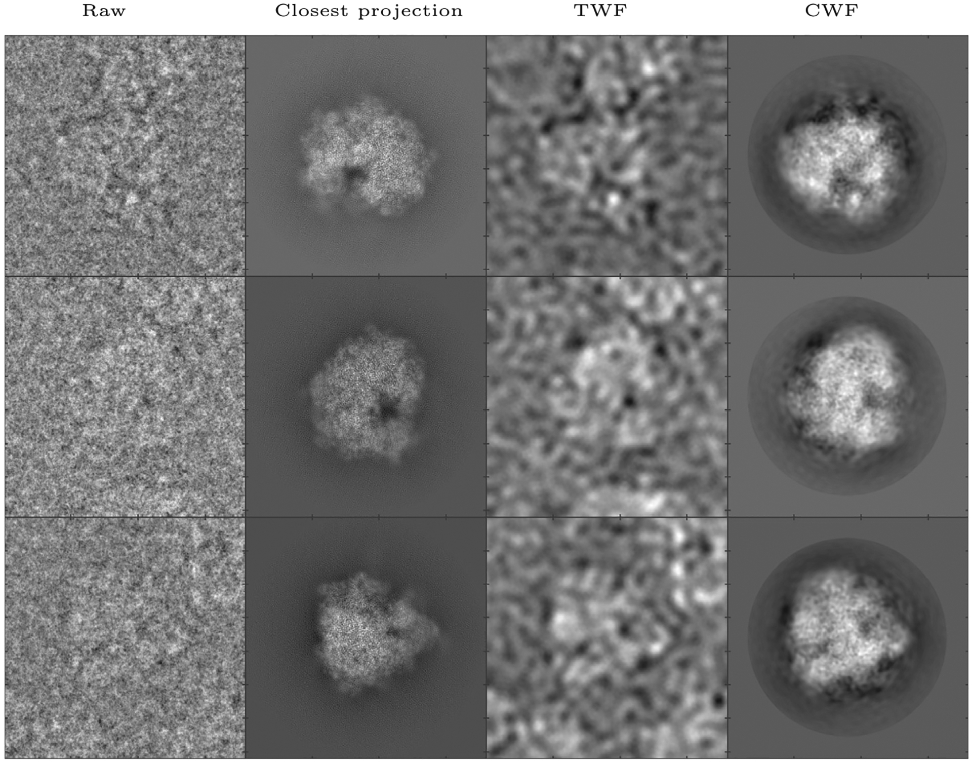
Denoising an experimental dataset of the 80S ribosome (Wong et al., 2014): Here we show, for three images in the dataset, the raw image, the closest true projection image generated from the 3D reconstruction of the molecule (EMDB 2660), the denoised image obtained using TWF, and the denoised image obtained using CWF. In this experiment, the first 30000 images out of the 105,247 images in the dataset were used for covariance estimation. The images are of size 360 × 360 and belong to 290 defocus groups. The amplitude contrast is 10%, the spherical aberration is 2mm, and the voltage is 300 kV.
3.5. Experimental dataset -
We apply CWF to an experimental dataset of the Inositol 1, 4, 5-triphosphate receptor 1(IP3R1) provided by Dr. Irina Serysheva, obtained using the older Gatan 4k × 4k CCD camera (Ludtke et al., 2011). The 3D reconstruction obtained from this dataset is available on EMDB as EMDB-5278. The dataset consists of 37,382 images of size 256 × 256 pixels with a pixel size of 1.81 Å. Using 20 cores, calculating the Fourier Bessel coefficients took 429 s while covariance estimation and Wiener filtering together took 589 s. The result is shown in Fig. 7. CWF retains 290 eigenvalues of .
Fig. 7.
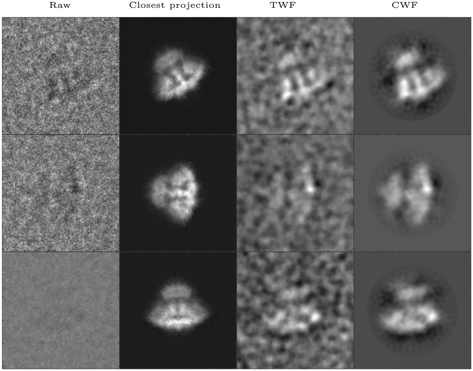
Denoising an experimental dataset of IP3R1 (Ludtke et al., 2011): Here we show, for three images in the dataset, the raw image, the closest true projection image generated from the 3D reconstruction of the molecule (EMDB 5278), the denoised image obtained using TWF, and the denoised image obtained using CWF. In this experiment, 37,382 images of size 256 × 256 belonging to 851 defocus groups were used. The amplitude contrast is 15%, the spherical aberration is 2 mm, and the voltage is 200 kV.
3.6. Experimental dataset −70 S ribosome
We apply CWF to an experimental dataset of the 70S ribosome provided by Dr. Joachim Frank’s group (Agirrezabala et al., 2012). This heterogeneous dataset consists of 216,517 images of size 250 × 250 pixels with a pixel size of 1.5 Å, obtained using the older TVIPS TEMCAM-F415 (4k × 4k) CCD detector. The 3D reconstruction obtained from this dataset is available on EMDB as EMDB5360. Using 20 cores, calculating the Fourier Bessel coefficients took 1174 s while covariance estimation and Wiener filtering together took 113 s. The result is shown in Fig. 8. CWF retains 219 eigenvalues of .
Fig. 8.
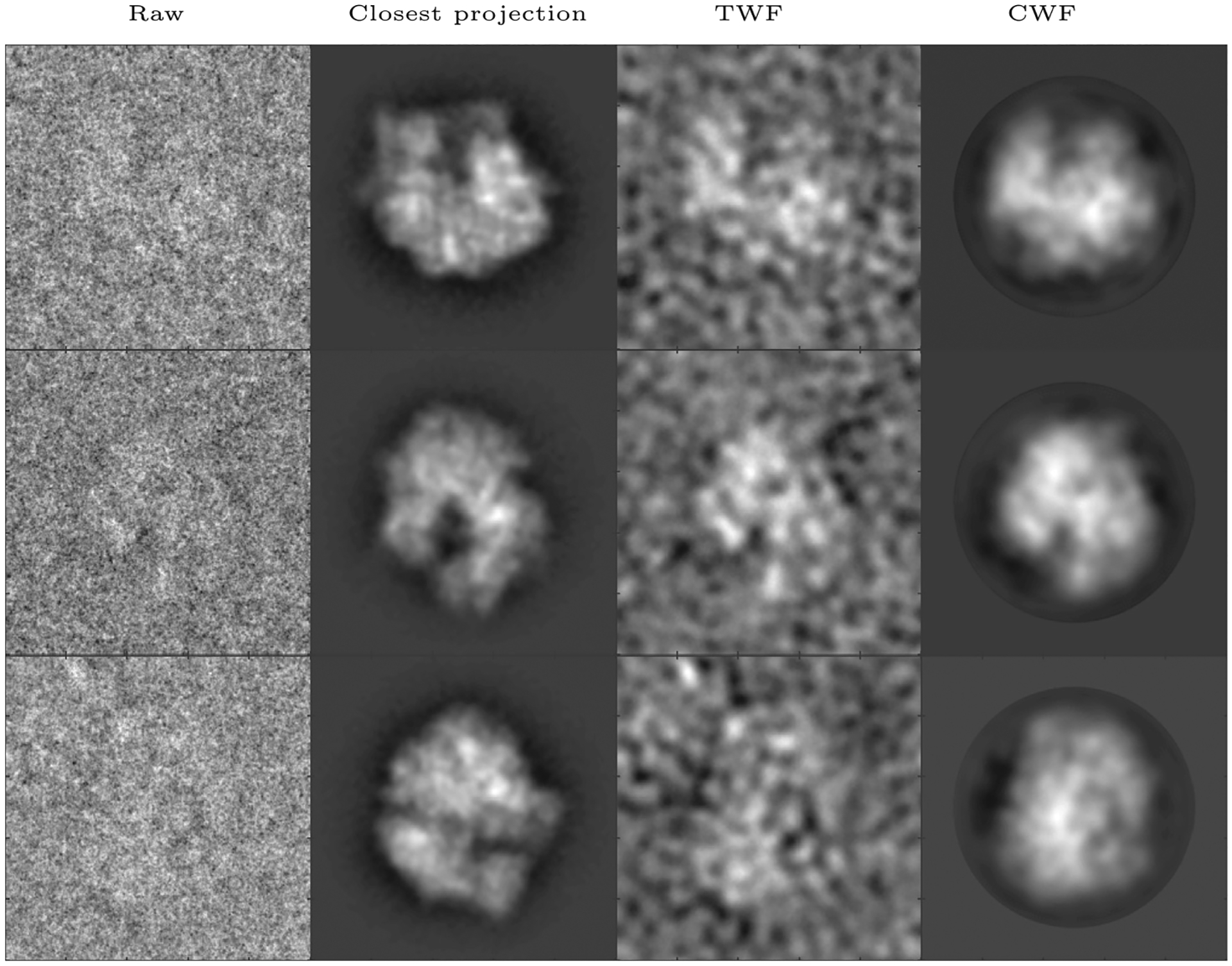
Denoising an experimental dataset of 70S (Agirrezabala et al., 2012): Here we show, for three images in the dataset, the raw image, the closest true projection image generated from the 3D reconstruction of the molecule (EMDB 5360), the denoised image obtained using TWF, and the denoised image obtained using CWF. In this experiment, the first 99,979 images out of the 216,517 images in the dataset were used for covariance estimation. The images are of size 250 × 250 and belong to 38 defocus groups. The amplitude contrast is 10%, the spherical aberration is 2.26 mm, and the voltage is 300 kV.
3.7. Outlier detection
In the cryo-EM pipeline, a significant amount of time is spent on discarding outliers by visual inspection after the particle picking step. CWF provides an automatic way to classify picked particles into “good” particles and outliers. The classifier uses the contrast of a denoised image to determine if it is an outlier.
The specimen particles can be at various depths in the ice layer at the time of imaging, so the acquired projection images can have different contrasts. The contrast can be modeled as an additional scalar parameter for each acquired noisy projection image as in Eq. (19), typically as a uniformly distributed random variable spread about its mean at 1.
| (19) |
We absorb the contrast into and estimate in this case, using the same procedure as before. We perform an experiment with synthetic data generated using EMDB-6454 with additive colored Gaussian noise at SNR = 1/20, and 10% of the projection images are replaced by “outliers”, that is, pure noise images containing no signal. Fig. 9c shows the estimated mean image , and Fig. 9d shows the top 6 principal components of the estimated covariance , also known as eigenimages. Fig. 9a and b show a sample of raw and denoised images respectively. High contrast images enjoy a higher SNR and are thus of interest for subsequent steps of the pipeline. On the other hand, outlier images, which typically have low contrast after denoising, can be automatically detected by a linear classifier after CWF and discarded from the dataset. In the experiment shown in Fig. 9a and b, a classifier with a threshold of 0.95 for the contrast discards 95% of the outliers, while 3% of the inliers are also discarded in the process.
Fig. 9.
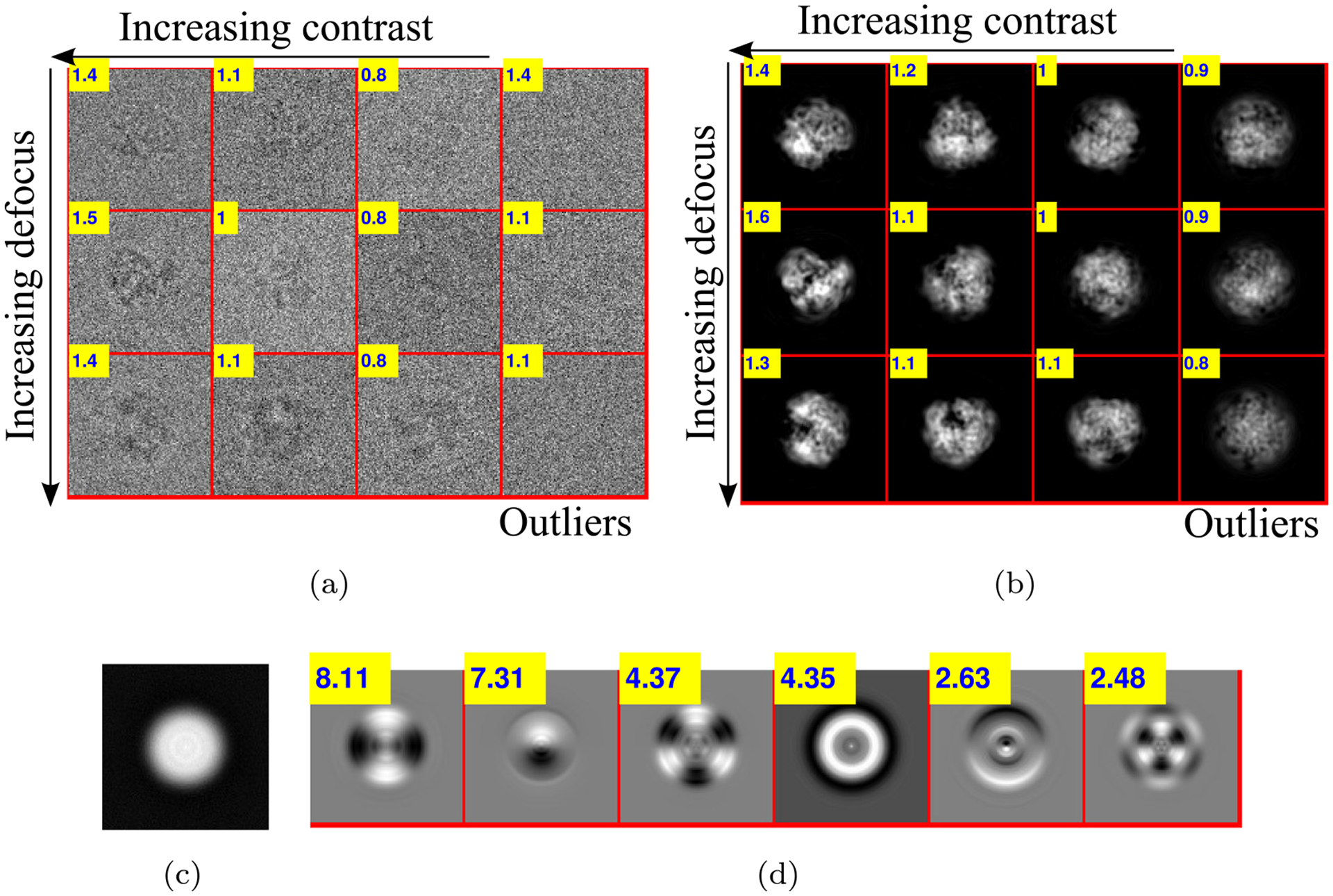
(a) Raw images: A sample of synthetic data generated using EMDB-6454 with additive colored Gaussian noise at SNR = 1/20.10% of the projection images are replaced by pure noise. The contrast parameter ranges from 0.75 to 1.5. The outliers are shown in the last column. Inset in a yellow box is the contrast of each image. (b) Denoised images: The denoised images using CWF. Notice the low contrast outliers in the last column. (c) Estimated mean image. (d) Top 6 eigenimages: Inset in a yellow box is the corresponding eigenvalue.
One can also use a different classifier based on features like the relative energy of the image before and after denoising, etc. However, outliers that look like particles, for example, images belonging to a different class of a heterogeneous dataset which act as “contaminants”, are difficult to detect using this method.
4. Conclusion
In this paper we presented a new approach for image restoration of cryo-EM images, CWF, whose main algorithmic components are covariance estimation and deconvolution using Wiener filtering. CWF performs both CTF correction, by correcting the Fourier phases and amplitudes of the images, as well as denoising, by eliminating the noise thereby improving the SNR of the resulting images. In particular, since CWF applies Wiener filtering in the data-dependent basis of principal components (“eigenimages”), while TWF applies Wiener filtering in the data-independent Fourier basis, we see in numerical experiments that CWF performs better than TWF, and considerably better at high noise levels. We demonstrated the ability of CWF to restore images for several experimental datasets, acquired with both CCD detectors and the state-of-the-art direct electron detectors.
Due to the high noise level typical in cryo-EM images, 2D classification is performed before estimating a 3D ab initio model. Class averages enjoy a higher SNR and are used to estimate viewing angles and obtain an initial model. For future work, it remains to be seen whether the resulting denoised images from CWF can be directly used to estimate viewing angles, without performing classification and averaging. Another possible future direction is integration of CWF into existing 2D class averaging procedures in order to improve their performance.
Acknowledgements
We are thankful to Maofu Liao, Sjors Scheres, Irina Serysheva and Joachim Frank for generously providing us with the experimental datasets. We thank Xiaochen Bai for answering our questions about the 80 dataset. We are grateful to Yoel Shkolniskly and Zhizhen Zhao for help with the code. We also thank Zhizhen Zhao for reviewing earlier versions of this manuscript, and for numerically expressing isotropic linear operators such as the CTF in the Fourier-Bessel basis. We thank Fred Sigworth and Joakim Andén for many helpful discussions about this work. We also thank Joakim Andén for pointing out the symmetrization required for the linear system to be solved by conjugate gradient. We are grateful to both reviewers and the editor for their helpful comments. The authors were partially supported by Award Number R01GM090200 from the NIGMS, FA9550-12-1-0317 and FA9550-13-1-0076 from AFOSR, LTR DTD 06-05-2012 from the Simons Foundation, and the Moore Foundation Data-Driven Discovery Investigator Award.
Footnotes
While in Eq. (9) is PSD, the new effective operator in the LHS of Eq. (11) is not necessarily PSD in general. In order to use conjugate gradient, we solve the system , where , in which the operator acting on in the LHS is PSD. is then obtained from the estimated .
In the case of astigmatism, where the CTF deviates slightly from radial isotropy this is a good approximation to obtain low resolution denoised images
References
- Agirrezabala X, Liao HY, Schreiner E, Fu J, Ortiz-Meoz RF, Schulten K, Green R, Frank J, 2012. Structural characterization of mRNA-tRNA translocation intermediates. Proc. Nat. Acad. Sci 109 (16), 6094–6099. 10.1073/pnas.1201288109, arXiv:http://www.pnas.org/content/109/16/6094.full.pdf, URL http://www.pnas.org/content/109/16/6094.abstract. [DOI] [PMC free article] [PubMed] [Google Scholar]
- Andén J, Katsevich E, Singer A, 2015. Covariance estimation using conjugate gradient for 3d classification in CRYO-EM. In: IEEE 12th International Symposium on Biomedical Imaging (ISBI), p. 200. 10.1109/ISBI.2015.7164051. [DOI] [PMC free article] [PubMed] [Google Scholar]
- Bai XC, McMullan G, Scheres SH, 2015. How cryo-EM is revolutionizing structural biology. Trends Biochem. Sci 40 (1), 49–57. [DOI] [PubMed] [Google Scholar]
- Bhamre T, Zhang T, Singer A, 2015. In: IEEE 12th International Symposium on Biomedical Imaging (ISBI), pp. 1048–1052. 10.1109/ISBI.2015.7164051. [DOI] [PMC free article] [PubMed] [Google Scholar]
- Box GEP, 1976. Science and statistics. J. Am. Stat. Assoc 71 (356), 791–799. 10.1080/01621459.1976.10480949, URL http://www.tandfonline.com/doi/abs/10.1080/01621459.1976.10480949. [DOI] [Google Scholar]
- Donoho D, Gavish M, Johnstone IM, Optimal shrinkage of eigenvalues in the spiked covariance model, CoRR abs/1311.0851 URL arxiv.org/abs/1311.0851. [DOI] [PMC free article] [PubMed]
- Frank J, 1996. Chapter 3 - Two-dimensional averaging techniques. In: Three-Dimensional Electron Microscopy of Macromolecular Assemblies. Academic Press, Burlington, pp. 54–125, URL http://www.sciencedirect.com/science/article/pii/B9780122650406500035. [Google Scholar]
- Frank J, Radermacher M, Penczek P, Zhu J, Li Y, Ladjadj M, Leith A, 1996. SPIDER and WEB: processing and visualization of images in 3D electron microscopy and related fields. J. Struct. Biol 116 (1), 190–199. [DOI] [PubMed] [Google Scholar]
- Kam Z, 1980. The reconstruction of structure from electron micrographs of randomly oriented particles. J. Theor. Biol 82 (1), 15–39. 10.1016/0022-5193(80)90088-0, URL http://idc311-www.sciencedirect.com/science/article/pii/0022519380900880. [DOI] [PubMed] [Google Scholar]
- Katsevich E, Katsevich A, Singer A, 2015. Covariance matrix estimation for the cryo-EM heterogeneity problem. SIAM J. Imaging Sci. 8 (1), 126–185. 10.1137/130935434, arXiv: 10.1137/130935434, URL 10.1137/130935434. [DOI] [PMC free article] [PubMed] [Google Scholar]
- Kritchman S, Nadler B, 2008. Determining the number of components in a factor model from limited noisy data. Chemometr. Intell. Lab. Syst 94, 19–32. 10.1016/j.chemolab.2008.06.002. [DOI] [Google Scholar]
- Kühlbrandt W, 2014. Cryo-EM enters a new era. eLife 3, e03678. 10.7554/eLife.03678, URL http://www.ncbi.nlm.nih.gov/pmc/articles/PMC4131193/. [DOI] [PMC free article] [PubMed] [Google Scholar]
- Liao M, Cao E, Julius D, Cheng Y, 2013. Structure of the TRPV1 ion channel determined by electron cryo-microscopy. Nature 504 (7478), 107–112. 10.1038/nature12822, URL http://europepmc.org/articles/PMC4078027. [DOI] [PMC free article] [PubMed] [Google Scholar]
- Ludtke S, Tran T, Ngo Q, Moiseenkova-Bell V, Chiu W, Serysheva I, 2011. Flexible architecture of IP3R1 by cryo-EM. Structure 19 (8), 1192–1199. 10.1016/j.str.2011.05.003, URL http://www.sciencedirect.com/science/article/pii/S0969212611001808. [DOI] [PMC free article] [PubMed] [Google Scholar]
- MacKay DJC, 2004. Chapter 46 - Deconvolution. In: Information Theory, Inference and Learning Algorithms. Cambridge University Press, Cambridge, UK, pp. 550–551 [Google Scholar]
- Marčenko VA, Pastur LA, 1967. Distribution of eigenvalues for some sets of random matrices. Math. USSR-Sbornik 1 (4), 457–483. 10.1070/sm1967v001n04abeh001994. [DOI] [Google Scholar]
- Milne JL, Borgnia MJ, Bartesaghi A, Tran EE, Earl LA, Schauder DM, Lengyel J, Pierson J, Patwardhan A, Subramaniam S, 2013. Cryo-electron microscopy - A primer for the non-microscopist. FEBS J. 280 (1), 28–45. [DOI] [PMC free article] [PubMed] [Google Scholar]
- Nogales E, 2016. The development of cryo-EM into a mainstream structural biology technique. Nat. Meth 13 (1), 24–27. 10.1038/nmeth.3694, Historical Commentary [DOI] [PMC free article] [PubMed] [Google Scholar]
- Park W, Chirikjian GS, 2014. An assembly automation approach to alignment of noncircular projections in electron microscopy. IEEE Trans. Autom. Sci. Eng 11 (3), 668–679. 10.1109/TASE.2013.2295398. [DOI] [Google Scholar]
- Penczek PA, 2010. Chapter two - Image restoration in cryo-electron microscopy. In: Jensen GJ (Ed.), Cryo-EM, Part B: 3-D Reconstruction, Methods in Enzymology, vol. 482. Academic Press, pp. 35–72, URL http://www.sciencedirect.com/science/article/pii/S0076687910820026. [DOI] [PMC free article] [PubMed] [Google Scholar]
- Sigworth FJ, Principles of cryo-EM single-particle image processing, Microscopy arXiv:http://jmicro.oxfordjournals.org/content/early/2015/12/23/jmicro.dfv370.full.pdf+html, doi: 10.1093/jmicro/dfv370. URL http://jmicro.oxfordjournals.org/content/early/2015/12/23/jmicro.dfv370.abstract. [DOI] [PMC free article] [PubMed] [Google Scholar]
- Sorzano C, Jonic S, Núñez-Ramírez R, Boisset N, Carazo J, 2007. Fast, robust, and accurate determination of transmission electron microscopy contrast transfer function. J. Struct. Biol 160 (2), 249–262. 10.1016/j.jsb.2007.08.013, URL http://www.sciencedirect.com/science/article/pii/S104784770700202X. [DOI] [PubMed] [Google Scholar]
- Sorzano CO, Vargas J, Otón J, Abrishami V, de la Rosa-Trevín JM, del Riego S, Fernández-Alderete A, Martínez-Rey C, Marabini R, Carazo JM, 2015. Fast and accurate conversion of atomic models into electron density maps. AIMS Biophys. 2 (20150102), 8–20. 10.3934/biophy.2015.1.8, URL http://www.aimspress.com/biophysics/article/198.html. [DOI] [Google Scholar]
- Tang G, Peng L, Baldwin PR, Mann DS, Jiang W, Rees I, Ludtke SJ, 2007. Eman2: An extensible image processing suite for electron microscopy. J. Struct. Biol 157 (1), 38–46. 10.1016/j.jsb.2006.05.009, software tools for macromolecular microscopy, URL http://www.sciencedirect.com/science/article/pii/S1047847706001894. [DOI] [PubMed] [Google Scholar]
- van Heel M, Harauz G, Orlova EV, Schmidt R, Schatz M, 1996. A new generation of the IMAGIC image processing system. J. Struct. Biol 116 (1), 17–24. [DOI] [PubMed] [Google Scholar]
- van Heel M, Gowen B, Matadeen R, Orlova EV, Finn R, Pape T, Cohen D, Stark H, Schmidt R, Schatz M, Patwardhan A, 2000. Single-particle electron cryo-microscopy: towards atomic resolution. Q. Rev. Biophys 33 (4), 307–369 [DOI] [PubMed] [Google Scholar]
- Wong W, Bai X-C, Brown A, Fernandez IS, Hanssen E, Condron M, Tan YH, Baum J, Scheres SH, 2014. Cryo-EM structure of the Plasmodium falciparum 80s ribosome bound to the anti-protozoan drug emetine. eLife 3, e03080. 10.7554/eLife.03080, URL http://www.ncbi.nlm.nih.gov/pmc/articles/PMC4086275/. [DOI] [PMC free article] [PubMed] [Google Scholar]
- Zhao Z, Singer A, 2014. Rotationally invariant image representation for viewing direction classification in cryo-EM. J. Struct. Biol 186 (1), 153–166. 10.1016/j.jsb.2014.03.003, URL http://www.sciencedirect.com/science/article/pii/S1047847714000549. [DOI] [PMC free article] [PubMed] [Google Scholar]
- Zhao Z, Shkolnisky Y, Singer A, 2016. Fast steerable principal component analysis. IEEE Transactions on Computational Imaging 2 (1), 1–12. 10.1109/TCI.2016.2514700. [DOI] [PMC free article] [PubMed] [Google Scholar]


