Accelerated multislice MRI with patterned excitation

Abstract

Purpose:

Accelerate multi-slice 2D MRI by using radiofrequency (RF) pulses that simultaneously act on different slices to combine contrast preparation and image acquisition.

Theory & Methods:

MRI applications often require the use of multiple RF pulses to generate desired contrast and prepare the signal for readout. Examples are the use of inversion pre-pulses to generate T₁ contrast, or the use of spin-echo (SE) preparations to generate T₂ or diffusion contrast. In multi-slice MRI, this separation of contrast preparation and readout can render scans time-inefficient and lengthy. We introduce a class of pulse sequences that overcomes this inefficiency by combining contrast preparation and signal readout. This is accomplished by using RF pulses that manipulate the magnetization of multiple slices simultaneously, and a gradient crusher scheme that selects a target slice for readout.

Results:

Feasibility of the method was demonstrated for spin-echo based measurement of water diffusion and tissue pulsation in human brain at 3 Tesla. Increases in time-efficiency and reductions in scan time were highly dependent on specific implementation and reached as high as 25% and 53% respectively.

Conclusion:

A novel approach to multi-slice MRI is demonstrated that reduces scan time for specific applications.

INTRODUCTION

MRI can flexibly generate a variety of contrasts to accentuate different aspects of tissue composition, physiology, and structure. This is done by a series of radiofrequency (RF) pulses and magnetic field gradient pulses that are played out in a specific sequence with specific timings. This pulse sequence serves to both manipulate the contrast, as well encode spatial information into the signal to generate an image. These two functions can be achieved sequentially, or concurrently.

Many of the early MRI applications were based on a sequential approach and generated T₁ and T₂ contrast with an RF inversion recovery or 90⁰-180⁰ RF spin echo (SE) preparation period (1). This approach continues to form the basis of many of the current clinical brain imaging techniques. For example, diffusion-weighted MRI uses a preparation phase that combines a 90⁰-180⁰ SE preparation with strong gradient pulses to create diffusion contrast (2,3). Typically, preparation is immediately followed by a localization segment where spatial information is encoded and MRI signal is collected (an ‘image acquisition’ segment). Generally, these methods allow excellent control of contrast but may be time inefficient as delays integral to signal preparation can be significant, so that a substantial fraction of the scan time is spent waiting for tissue contrast to establish and not acquiring data.

On the other hand, steady state free precession (SSFP) is a class of techniques (4–9) that performs both functions concurrently and has improved time-efficiency; however the contrast generated is often more difficult to interpret and generally sub-optimal. This is in part due to the various types of NMR echoes that contribute to the SSFP signal and determine image contrast (10).

In the following, we describe a new class of imaging methods that offers high time efficiency while also allowing excellent control of contrast. Application to the measurement of water diffusion and tissue pulsations is demonstrated in human brain at 3 Tesla.

THEORY

The new approach, here referred to as “Patterned Multi-slice Excitation” (PME) MRI, is an adaptation of multi-slice MRI that allows for more time-efficient generation of contrasts that require more than one RF pulse to generate, including SE- and stimulated echo (STE)-based techniques. Of note, the term ‘excitation’ in our description of PME is used liberally to include any proton spin rotation, including the generation and refocusing of transverse magnetization, and the inversion of longitudinal magnetization. PME changes each RF pulse’s excitation pattern to not just act on a single target slice, but also manipulate (‘prepare’) the magnetization of upcoming slices in the multi-slice acquisition sequence or ‘slice acquisition protocol’. Therefore, while acquiring data for a specific slice, the magnetization of upcoming (‘to-be-imaged’) slices is altered to provide a way of generating contrast in a time-efficient manner. The slice pattern targeted with each RF pulse, together with the slice acquisition protocol (i.e., the temporal order of scanning the individual slices in the slice stack), dictates the sequence of RF pulses that each slice experiences in succession and provides flexibility in generating the desired contrast. As each RF pulse is followed by image acquisition, it increases time efficiency compared to standard SE and STE MRI by reducing the number of exclusive RF pulse intervals required for each slice. Unlike SSFP, it allows strict control of the types and number of echo signals that contribute to each image.

Applied to the measurement of SE signals, PME allows substantial shortening of scan time compared to conventional SE MRI (Figure 1). The latter requires two RF pulse intervals to acquire data for a single slice, with one RF pulse exciting a given slice to convert longitudinal magnetization into transverse magnetization, followed by dephasing period, and a subsequent, delayed, second pulse serving to refocus this magnetization (Figure 1a), followed by a rephasing and acquisition period. With PME, each RF pulse performs these two functions for two separate slices in the slice acquisition protocol at once (Figure 1b): One component of the RF pulse refocuses the target slice, while a second component excites an upcoming slice in the acquisition protocol. Thus, what otherwise would require a separate dephasing and rephasing/acquisition interval for each slice, is accomplished more efficiently by collapsing these two segments into one and still produce the desired SE-type contrast. As a result, the slice-to-slice repetition time (sTR) is reduced. An important element in this approach is the gradient crusher following the RF pulse, which serves to both eliminate (‘dephase’) signal originating from outside the target slice and refocus the SE signal that has been excited in a previous interval.

Figure 1.

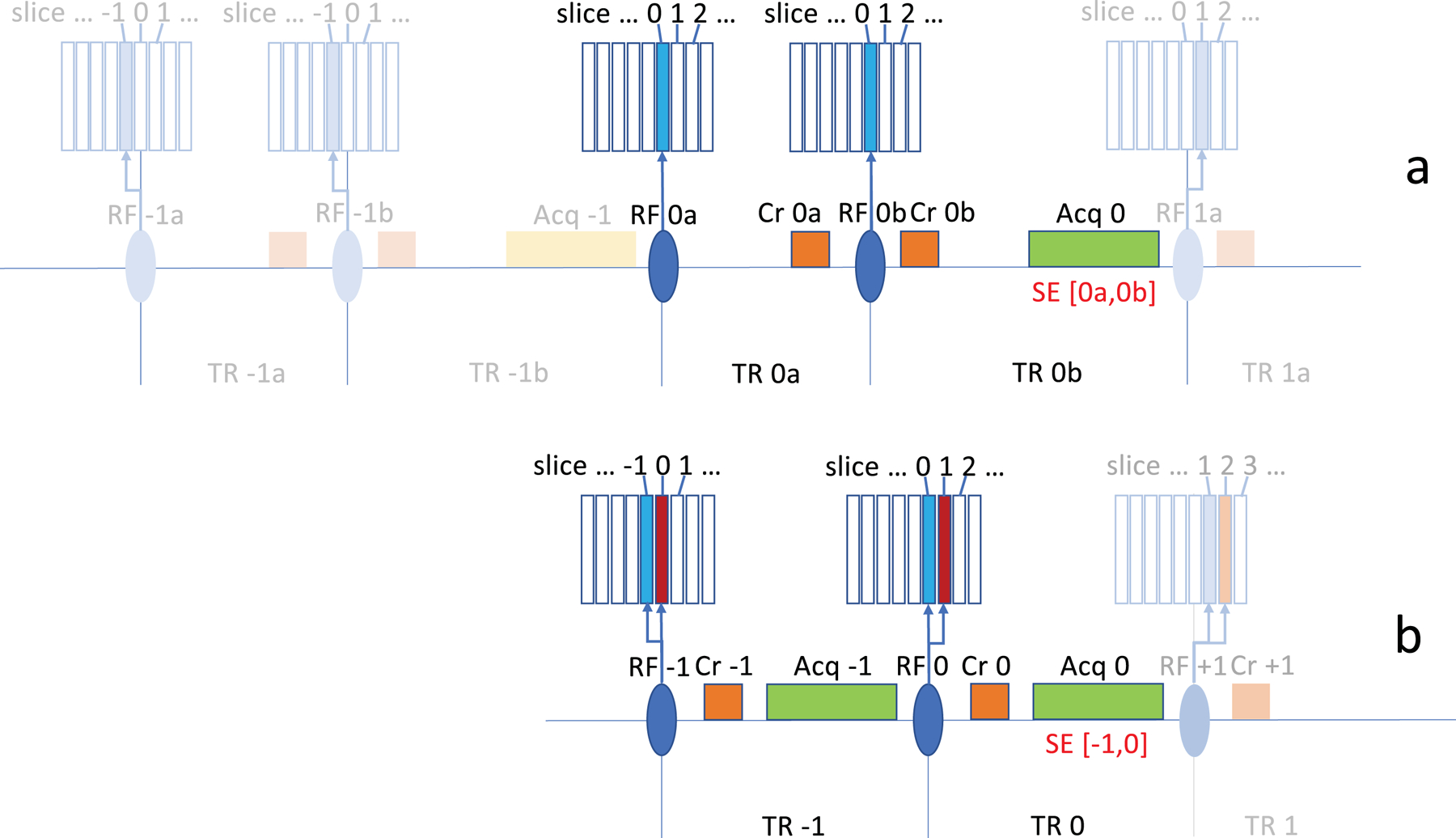
Basic principle of patterned multi-slice excitation exemplified with 2-slice excitation for SE acquisition. In conventional sequential multi-slice acquisition for spin echo MRI (a), two RF pulse intervals ‘TR na’ and ‘TR nb’ (following ‘RF na’ and ‘RF nb’) are used to acquire data for a specific slice (‘Acq n’). Two gradient crushers (‘Cr na’ and Cr ‘nb’) are used to eliminate gradient echo signals and select the spin echo (SE) signal. This signal is indicated as ‘SE [na,nb]’, a spin echo signal that results from pulses ‘RF na’ and ‘RF nb’. On the subsequent repetitions in this example, the slice location is shifted by one slice width based on a sequential slice acquisition protocol, and the slice repetition time (sTR) is the sum of ‘TR na’ and ‘TR nb’. In a patterned multi-slice excitation (b), the target slice ‘n’ is refocused while one additional slice is excited (‘n+1’, red), to be acquired in the subsequent pulse interval. Acquisition in each interval ‘n’ is preceded by a crusher ‘Cr n’ which suppresses gradient echo (GE) signals, and leads to the generation of just a SE signal from pulses in intervals ‘n-1’ and ‘n’, indicated as ‘SE [n-1,n]’. Using a sequential slice acquisition protocol as with the conventional approach, the pattern is shifted by one slice width on subsequent repetitions. The slice repetition time is equal to a single pulse interval TR. Slice select gradients (not shown here) accompany the RF excitations.

Flip angles or slice thicknesses do not need to be identical for the two slice excitations performed within each RF pulse. RF pulses can be designed to use a 180°−90° combination to maximize the SE signal. Excitation of the set of slices with each repetition can but does not need to be accomplished with a single RF pulse. Excitation can be done sequentially using multiple pulses, which allows shifting of the SE refocusing time (‘echo top’) relative to the image acquisition window (Figure S1).

Many variants are possible, for example the two excited slices in the case of the sequential acquisition protocol above can be separated in space to increase T₂-weighting. This increased spatial separation would increase the time between when a slice experiences the 90° and 180° pulses (e.g. from 1 to 2 sTR), and subsequently also the echo time at which the signal is observed (in this example in the 4^th instead of the 2^nd interval after the 90° pulse).

Furthermore, with each RF excitation, more than two slices can be excited simultaneously, resulting in spins within the same slice experiencing more than two RF pulses during execution of the slice acquisition protocol. The temporal order in which they experience these pulses is counter to the order of the excitation pattern in the slice acquisition table. For example, a [180⁰, 90⁰] pattern in the acquisition table (meaning applying a flip angle of 180^o to slice n in the table as well as a flip angle of 90^o to slice n+1) is experienced as a 90⁰-180⁰ temporal RF pulse sequence. Three pulse variants can for example be used to generate a stimulated echo (STE). A stimulated echo with a mixing time (TM) of two TR periods (Figure 2) can be generated by using a [90°, 0°, 90°, 90°] excitation pattern in the slice acquisition table (applying flip angles of 90°, 0°, 90°, 90° to slices n, n+1, n+2, and n+3 respectively on repetition n). Specificity to the STE signal by reducing contributions of other signals is possible by using flip angles close to 90⁰ and by varying gradient crusher moment and/or direction on subsequent pulse intervals (see Table S1).

Figure 2.

Example of stimulated echo (STE) generation with a 3-slice excitation pattern ‘x0xx’. In addition to the slice under study, an adjacent slice as well as a slice 3 slice positions over is excited. As a result, in each pulse sequence interval ‘n’, a stimulated echo is generated that has seen pulses at ‘n’, ‘n-1’, and ‘n-3’, indicated as ‘STE [n-3, n-1, n]’. The single slice gap (‘null excitation’) leads to lengthening of the STE TM by one TR, increasing from 1 to 2 TRs.

Longer TE or TM and periods can be generated by having one or more of the pulses affecting slices longer in advance of their time of acquisition. This may need to be accompanied by a modified gradient crusher modulation pattern (Table S1). Three-pulse sequences can also be used to generate an SE signal with inversion-recovery or saturation-recovery weighting, for example by generating a [180°, 90°, 180°] or [90°, 90°, 180°] excitation pattern.

Several initial applications are envisioned. For example, similar to 3D SSFP-based diffusion MRI (for review see (11)), a large crusher amplitude can be used to introduce diffusion contrast. Unlike diffusion-weighted (DW) SSFP, the proposed PME approach applied to STE acquisition (Figure 2) allows long TM STEs to be selectively generated, increasing diffusion contrast and its interpretation: Since a specific signal pathway is selected in PME, the accurate diffusion weighting factor (‘b-value’) can be computed. Similarly, using a large crusher in the PME SE example shown above introduces diffusion contrast and allows diffusion-weighted MRI with high time-efficiency: A slice is scanned for each RF pulse interval. Sample DW imaging implementations are discussed below.

The use of large crusher gradients in SE and STE MRI also increases sensitivity to subtle tissue displacement, and has particularly strong effects on image phase. This has been exploited with techniques like DENSE (displacement encoding with stimulated echoes) and SSFP for the measurement of brain pulsations and elastography (8,12–14). Below we show that this may be more efficiently done with the PME concept using an SE approach (Figure 1b).

METHODS

PME MRI was implemented and evaluated on a 3 T Siemens Prisma (Siemens Healthineers, Erlangen, Germany) equipped with a 32-channel head coil and an AS82 gradient set with a maximum amplitude of 80 mT·m⁻¹ and 200 T·m⁻¹·s⁻¹ maximum slew rate. Gradient duty cycle was limited to about 35% at the maximum gradient strength of 52 mT·m⁻¹ we used in the applications described below. A pulse-oximeter signal, recorded with a BIOPAC MP150 system (Biopac, Goleta, CA, USA), served as an indicator of cardiac phase for the analysis of brain pulsations induced by the cardiac cycle (see below).

Scans were performed on n=19 healthy volunteers (14 female, 5 male, aged 29.4 ± 8.8 years) under an IRB-approved protocol. Anatomical reference scans were performed with sagittal MPRAGE at 1 mm isotropic resolution. Sixteen of these volunteers were scanned with the displacement imaging protocol. The diffusion protocol, which took us longer to develop, was acquired on 5 subjects, 2 of which were also scanned with the displacement imaging protocol.

The PME implementation evaluated here used an EPI readout after a crusher gradient and used 2- and 3-slice excitation versions analogous to Figures 1b and 2, for SE and STE implementations, respectively. For the STE implementation, the gradient crusher was modulated in direction over repetitions (sTRs) to eliminate SE signals (analogous to Table S1, see below). For the SE implementations, the gradient crusher’s amplitude or direction was only varied over volume repetitions (vTRs). Depending on the application, crushers also served to generate tissue displacement or diffusion contrast. The crushers gradient’s effective direction provided sensitization to different water diffusion or tissue displacement directions (see below). All applications use an interleaved slice acquisition protocol. This facilitated the incorporation of lipid suppression, accomplished by alternating the slice frequency offset and slice select gradient polarity on subsequent excitations (15,16).

PME was accomplished by combining a slice selection gradient with a frequency modulated pulse similar to that used in simultaneous multi-slice (SMS) MRI (17). PME excitations extending beyond an edge of the slice stack were adjusted to properly excite slices at the opposing edge, i.e., their center frequencies were cyclically adjusted. This avoided having some of slices not experiencing the full excitation sequence on the upcoming scan repeats through the slice stack. Only data from the first n sTRs in the experiment contained no signal, where n is 1 for SE [−1,0], and as high as 6 for the STE [−6,−5,0] example discussed below.

Measurement of brain tissue pulsations associated with the cardiac cycle

Vascular pulsations with the cardiac cycle lead to subtle brain tissue movement that can be measured with phase contrast MRI using spin echoes or stimulated echoes (18,19). PME has the potential to increase scan speed and facilitate capturing the complex spatio-temporal patterns of this movement. To demonstrate this, we implemented a 2-slice PME excitation generating an SE, combined with crusher gradients of 150 ms·mT·m⁻¹. This was achieved with a crusher amplitude and duration of 52.1 mT·m⁻¹ and 2.88 ms, respectively. The required [180°, 90°] PME pattern in the interleaved acquisition table required a [180°, 0°, 90°] PME spatial pattern. For this purpose, a 4 ms long PME pulse with time-bandwidth product (TBWP) of 4 was used for the 90° component (excitation) of the pulse. The time-bandwidth product for the 180° (refocusing) component of the pulse was increased to 5.2, yielding a 30% thicker refocusing slice thickness for the given slice select gradient amplitude. This served to minimize undesirable signal losses from slice profile imperfections and off-resonance, considering the use of alternating slice select gradient polarity over shots (for lipid suppression).

Image readout was performed with single shot EPI with 2 mm isotropic resolution using rate-3 SENSE acceleration (20). Fourty-nine axial-oblique slices were collected with 25% slice gap along the AC-PC direction, using 63 ms TE (at center of EPI acquisition window) an sTR of 40 ms (1960 ms vTR) and rate-3 SENSE acceleration (21), see also Table 1. Acquisition bandwidth was 250 kHz, matrix size was 120×90 over 240×180 mm² field-of-view. Multiple (n=200) repetitions were collected for each of 3 orthogonal crusher orientations (in separate scans) in order to abundantly sample the full range of possible delays between cardiac systole and the displacement-sensitive period of each acquired slice (16). This resulted in a total scan time of 392 s for each of three experiments sensitive to three orthogonal displacement directions.

Table 1.

Scan parameters and resulting diffusion b-values for the various scans used in this experiment.

	Diffusion imaging									Displacement encoding
resolution [mm3]	3.03			2.53			2.03			2.03
scan type	conventional SE	PME SE	PME STE	conventional SE	PME SE	PME STE	conventional SE	PME SE	PME STE	PME SE
volume TR (vTR) [ms]	3800	1800	1376	4200	2021	1645	4900	2444	2068	1960
slice TR (sTR) [ms]	84.4	40.0	32.0	89.4	43.0	35.0	104.3	52.0	44.0	40.0
number of slices	45	45	43	47	47	47	47	47	47	49
TE [ms]	59.8	66.5	50.4	63.0	72.1	55.3	70.2	84.0	68.3	63.0
EPI train length [ms]	15.31			20.88			30.60			24.96
crusher moment high / low [ms·mT·m−1]	801.8 / 40.0	656.9 / 30.0	285.0 / 30.0	776.2 / 40.0	626.0 / 30.0	275.0 / 40.0	737.8 / 50.0	570.0 / 40.0	245.0 / 50.0	150.0 / -
crusher amplitude high / low [mT·m−1]	46.2 / 2.3	45.6 / 2.1	44.9 / 4.7	46.2 / 2.4	45.5 / 2.2	44.6 / 6.5	46.2 / 3.1	45.2 / 3.2	43.9 / 9.0	52.1 / -
crusher duration (δ) [ms]	16.36	14.40	6.35	16.81	13.77	6.17	15.98	12.61	5.58	2.88
crusher spacing (Δ) [ms]	29.36	40.00	160.00	30.34	43.00	175.00	33.56	52.00	220.00	40.00
b-value high / low [s·mm−2]	1157 / 3	1136 / 2	1113 / 12	1135 / 3	1131 / 3	1136 / 24	1162 / 5	1157 / 6	1134 / 47	64 / -

Measurement of water diffusion

Two and three-slice PME implementations analogous to Figures 1b and 2 respectively were used to generate SE- and STE-based diffusion contrast. For the SE implementation, diffusion weighting was varied by changing crusher amplitude and/or direction on successive vTRs according to a 12-direction cycling scheme and 2 b-values (b=1157 an b=5.7 s·mm⁻²). The cycling was repeated multiple times (n=32 for low-b and n=180 for high-b) to evaluate the required number of averages to derive parametric maps. Crusher durations of 12.61 ms were used with amplitudes of 45.2 mT·m⁻¹ and 3.2 mT·m⁻¹ for high- and low-b diffusion weightings, respectively. Other parameters include 84.0 ms TE (center of the EPI acquisition window), 52 ms sTR, 2444 ms vTR, isotropic 2 mm resolution, 30.6 ms EPI readout duration using 250 kHz acquisition bandwidth, 47 axial-oblique slices along AC-PC direction, using 20% slice gap, and rate-2 SENSE acceleration. Matrix size was 120×90 over 240×180 mm² field-of-view.

For comparison, conventional (no PME) SE DW MRI was performed as well using identical EPI readout, 70.2 ms TE and 104.2 ms sTR. The TE was the minimum possible to approximately yield the same diffusion b-value as used in the PME-SE. The sTR was then set to the minimum as dictated by the gradient duty cycle limits.

Lower spatial resolution acquisitions were performed as well: A 2.5 mm isotropic resolution (96×72 matrix) PME SE version with 1131 s·mm⁻² high- and 2.6 s·mm⁻² low-b values, and a 3 mm isotropic resolution version (80×60 matrix) with 1136 s·mm⁻² high- and 2.3 s·mm⁻² low-b value. Echo times were 71.2 and 66.5 ms for 2.5 and 3.0 mm resolutions, respectively, sTRs were 43.0 and 40.0 ms. The equivalent conventional SE DW MRI used respectively 63.0 and 59.8 ms TE, and 89.4 and 86.7 ms TR at those same 2.5 and 3.0 mm resolutions, respectively. Only 6 diffusion directions were used in 3-mm acquisitions. Other parameters are as listed above; Table 1 gives an overview and additional details.

A 3-slice PME excitation was used to evaluate STE-based DW MRI with a 5 sTR TM period. This requires a 90°−90°−0°−0°−0°−0°−90° order of RF excitations and thus a [90°, 0°, 0°, 0°, 0°, 90°, 90°] PME pattern in the slice acquisition table. EPI acquisitions were performed at the 2, 2.5 and 3 mm isotropic spatial resolutions as above, with crusher duration and amplitude of 5.58 ms and 43.91 mT·m⁻¹ respectively, at 2 mm resolution. (Note that the substantially longer diffusion time in PME STE DW MRI required shorter duration gradients to achieve similar b-value.) Other parameters include 68.3 ms TE and 44.0 mm sTR. Again, cyclical excitation was performed to avoid incomplete excitations at the beginning of the slice stack. A six-direction diffusion weighting scheme was used for all STE resolutions. In contrast to the SE implementation, cycling through this scheme was performed on successive pulse intervals (sTRs). This in effect resulted in the diffusion gradients simultaneously generating diffusion weighting as well as implicitly suppress unwanted SE signals (Figure S2). On successive repetitions of the slice stack, the same slice received a different diffusion weighting to ensure each slice was sampled at the full set of possible diffusion weightings. To this end, the number of slices was chosen not to have any common factors with the number of diffusion directions, so that the sequence of directions could be continued in a cyclical manner over the MR volume repetitions.

Data analysis

Data was analyzed with IDL v8.8.3 (Harris Geospatial, Broomfield, CO, USA). For tissue pulsation measurements, images were first registered to the last volume in the acquired series with an encoding gradient in the readout direction (in-plane registration only, to avoid mixing data from different slices, and therefore different cardiac phases). The registration was based on image magnitude, after which the rotation and translation findings were applied to the complex data. For each slice independently, 50% of the repetitions that showed the smallest phase change over repetitions was identified, thus identifying a subset of data minimally affected by cardiac pulsatile effects. Voxel-wise trends (up to 4^th order polynomial) were then computed using that most-stable 50% of the data. After spatial smoothing (Gaussian, 4 voxels) of the fitted trends, the trends were removed from all timeseries data. This included temporal mean phase, predominantly originating from B₀ inhomogeneity. Subsequently, images were sorted according to their time of acquisition as compared to the preceding peak of systole as estimated from the pulse-oximeter signal. For this purpose, the latter was time shifted by −250 ms to provide an approximate correction for its delay with ECG (22). Note that this does not account for the latency between cardiac beat and arrival of the resulting blood pressure wave in the brain.

Acquisition timing relative to the nearest subsequent heartbeat was also extracted from the pulse-oximeter measurement, which allowed inclusion of a second copy of the data in this sorted set. This allowed for calculating the signal at negative latency values. As the heartbeat is not strictly periodic, this procedure is expected to give more accurate results for displacement values immediately prior to the heartbeat than equating these to the results at long latency times.

To filter out outliers, the sorted data were compared to a temporally convolved (Gaussian weighting function, width chosen to achieve averaging over approximately 10 samples) version of the sorted data, based on which outliers were identified as exceeding 2.5 SD in the difference between filtered and unfiltered sorted data. Remaining data were thereafter again convolved with a Gaussian weighting function for averaging purposes, typically with a full width at half maximum of 0.1 s. Both convolutions accounted for the non-equidistant sampling resulting from the sorting of the data.

Diffusion data was analyzed based on EPI magnitude images. Voxel-wise mean diffusivity (MD), fractional anisotropy (FA), diffusion tensor matrix and fiber orientation maps were generated as described in (23).

To allow comparison of the sensitivity of the three diffusion imaging methods, relative temporal signal-to-noise ratio (tSNR) and relative temporal variance (each accounting for differences in vTR) in each experiment was computed for each voxel in an ROI that approximately covered white matter. This ROI was defined as voxels in the brain in which fractional anisotropy exceeded 0.25 for all three experiment types (conventional SE, PME SE and PME STE) at that spatial resolution. For high-b data, temporal SNR is computed per diffusion direction (12 directions for 2.0 and 2.5 mm data; 6 for 3.0 mm data), and then averaged over diffusion directions and voxels. A single tSNR value per voxel is calculated for the low-b data in the same ROI, and then averaged over voxels. Results are subsequently corrected for the volume TR to yield tSNR per unit time. The resulting mean value per volunteer is then normalized to the value found for the conventional SE diffusion experiment for that volunteer and resolution.

RESULTS

Brain tissue pulsations

Sample results for PME-based measurement of brain tissue pulsations with the cardiac cycle are shown in Figure 3, Figure 4 and Figure S2. Results show good qualitative correspondence to previous reports (14,18). In-plane, a centropetal displacement following systole was observed that reached 20–50 µm for each 40 ms sTR and lasted 100–200 ms, leading to an estimated total displacement of 100–200 µm (Figure 4). Through-plane, displacement following systole was most prevalent in the head-to-foot direction and strongest near the center of the most inferior slices (Figure S2). To illustrate robustness of the method, results for the same slice taken from the data acquired with left-right encoding, for all volunteers (n=16), are shown in Figure S3.

Figure 3.

Tissue displacement with cardiac cycle measured with PME SE according to Figure 1b. A single slice out of the 49-slice stack is shown (MPRAGE and the first EPI image shown at the top). Cardiac-timing dependent displacement as a function of displacement encoding direction is shown, in µm per sTR (40 ms in these experiments). Top row: Anterior-posterior (AP) encoding; Second row: Left-right (LR) encoding; Third row: head-foot (HF) encoding. Bottom row: Total displacement per sTR, is calculated as the root-mean squares combination of the three encoding directions. An approximation of the outline of the brain, in red on the left-most image in each row, was extracted from the MP-RAGE anatomical reference volume.

Figure 4.

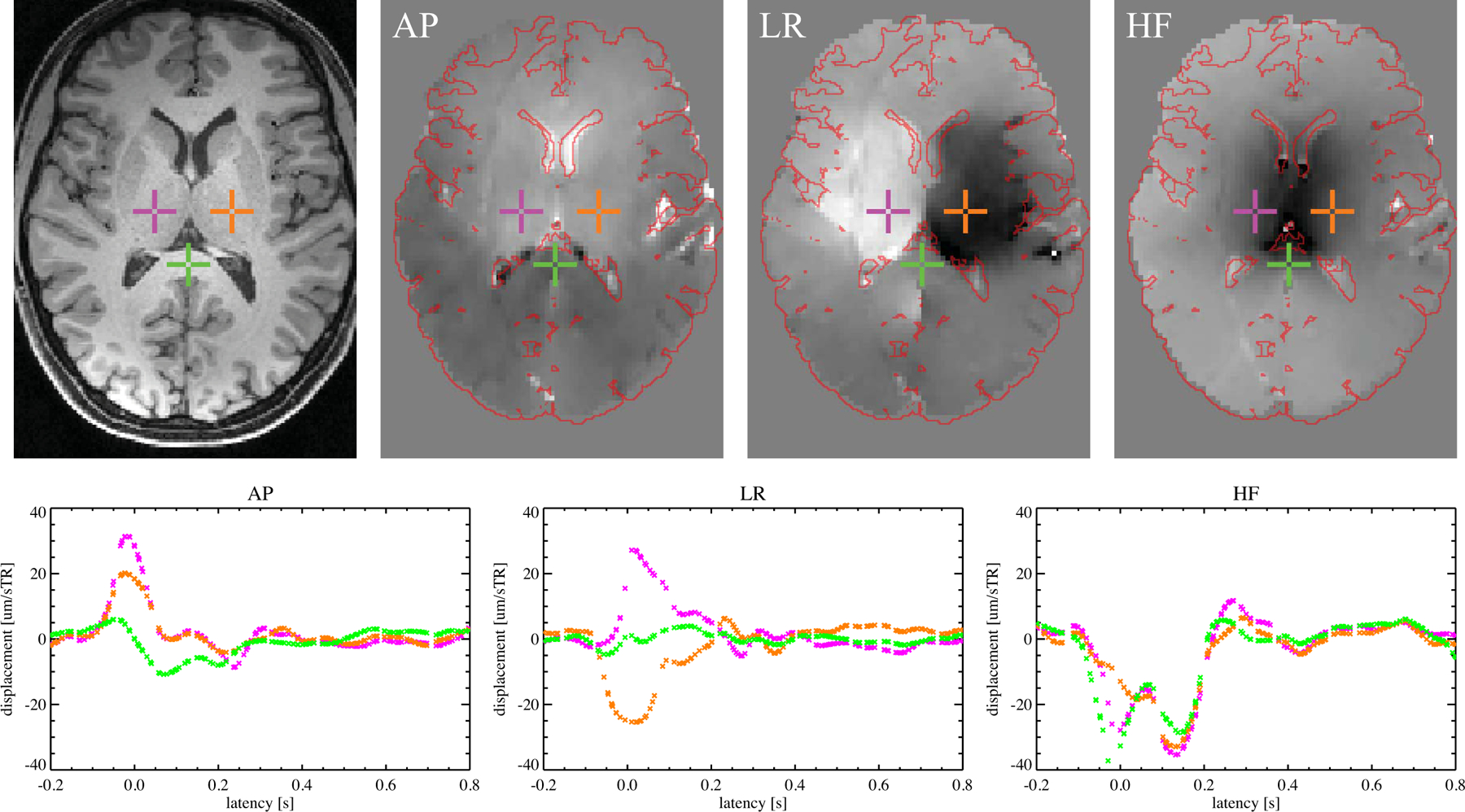
Tissue displacement as a function of latency with respect to cardiac event for three voxels from a single slice. Anatomical reference (left) and displacement maps for this slice for the 0.0–0.1 s latency bin from the experiments with gradient in AP, LR and HF directions are shown in the other three panels in the top row. (Displacement grayscale range was ±25, ±25 and ±40 µm per sTR, respectively, for the AP, LR and HF maps. Approximate brain outline, in red, was extracted from localizer.) For three voxels, highlighted using colored crosses in the top row, the displacement as a function of latency is shown in plots in the bottom row, using the same colors, for respectively a gradient in the AP, LR and HF directions.

Diffusion-weighted MRI

Sample results for PME-based measurement of water diffusion are shown in Figures 5 and 6. Figure 5 shows diffusion direction, FA and MD for 8 out of 47 slices for one of the 2.0 mm resolution PME SE datasets. Across parameter settings, high quality maps of diffusion direction were obtained for both STE and SE PME approaches that showed good qualitative correspondence to conventional (non-PME) technology (Figure 6). For the PME SE data a 3 mm resolution, SNR of the individual DW maps was sufficiently high to allow good quality MD, FA and diffusion direction maps with as little as 13 s worth of data (combining 6 b=1136 s·mm⁻² maps + 1 b=2.3 s·mm⁻² map). PME STE data could be acquired even faster, in under 10 s for the 7 shots required, but at the cost of a notable sensitivity loss.

Figure 5.

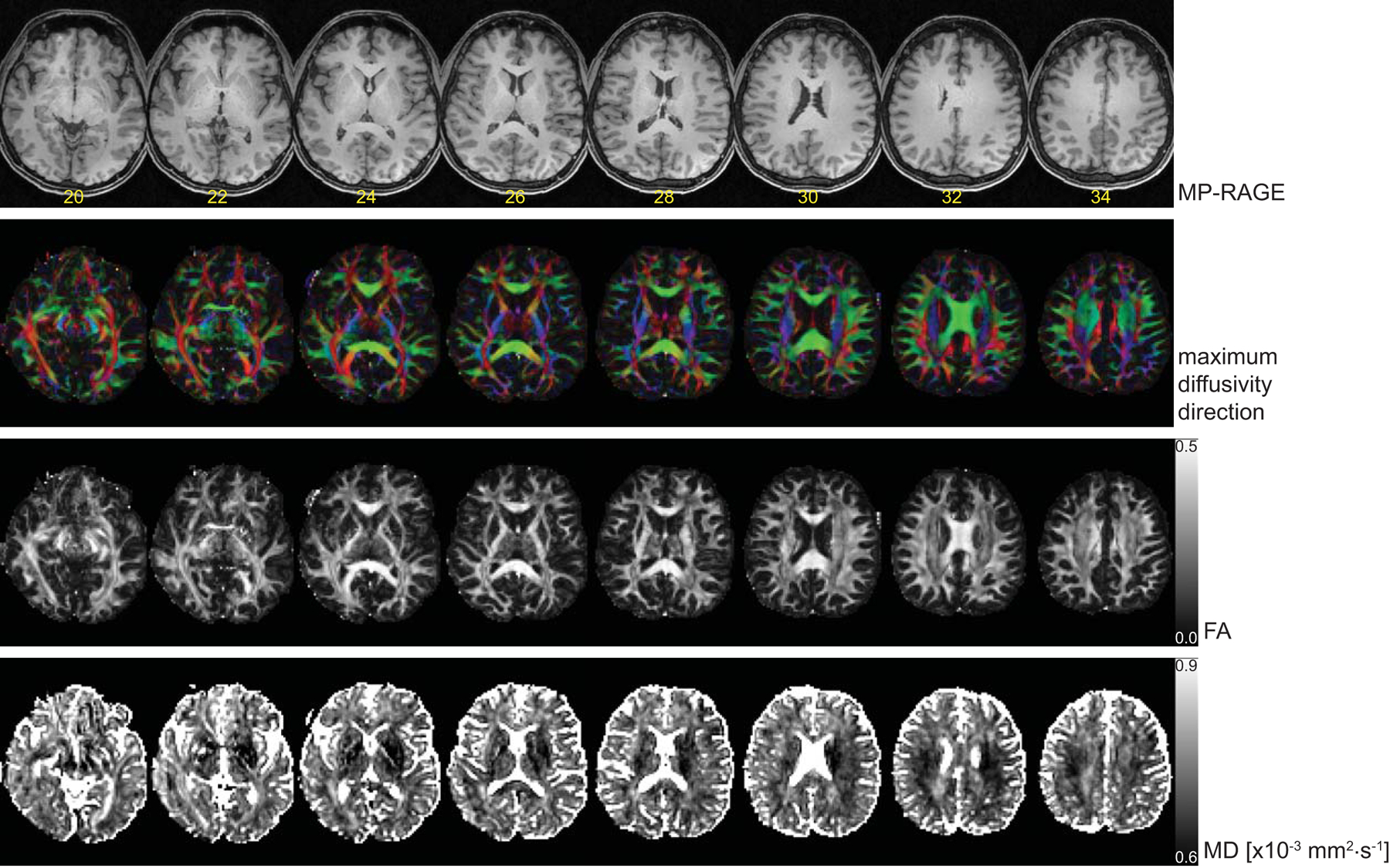
Sample results for 2 mm resolution PME SE DW MRI. Top row shows MPRAGE localizer with slice number superimposed. Second row: The diffusion direction color maps. Third row: Fractional anisotropy (FA) maps. Bottom row: Mean diffusivity (MD).

Figure 6.

DW PME MRI with SE and STE acquisition schemes compared to conventional DW SE MRI. Top left: Anatomical localizer. Top row: Diffusion direction color maps at 3.0 mm isotropic resolution. Middle row: 2.5 mm isotropic resolution. Bottom row: 2.0 mm isotropic resolution. Acquisition time for the data used as the basis for each map is printed below each image (format mm:ss). At 3.0 mm resolution, PME SE MRI has sufficient sensitivity to allow acquisition of orientation maps in as little as 13 seconds. Equivalent conventional SE MRI requires about 27 s for this resolution. STE-based PME DW MRI can be performed even faster, in 10 seconds in this example, but at the cost of approximately a two-fold SNR loss associated with stimulated echo generation. MPRAGE for this slice is shown in the top-left, the three remaining columns show PME SE, PME STE and conventional SE based diffusion data.

Quantitative comparison of tSNR per unit time (Table 2) showed a favorable performance of PME SE versus conventional SE as well, with improvements ranging between 13% and 38%. PME STE showed inferior performance compared to both SE versions. This is attributed to the approximately 50% signal loss associated with stimulated echo signal generation. A more detailed analysis of the signal variance in these diffusion data can be found in Figure S4 and Table S2. To demonstrate that PME also allows notably higher b-values to be used, yielding equivalent performance in a comparison with conventional SE, one set of 2.5 mm isotropic resolution experiments with a b-value of approximately 2500 s·mm⁻² was performed, see Figure S5.

Table 2.

Relative temporal SNR (tSNR) per unit time for PME SE and PME STE when compared to the conventional SE diffusion experiment at the same resolution. Results are mean ± standard error over volunteers (n=5) after averaging over voxels in an ROI that approximately covers white matter in the various experiments.

Resolution [mm]	PME SE		PME STE
	low-b	high-b	low-b	high-b
3.0	1.25 ± 0.02	1.38 ± 0.08	0.79 ± 0.03	0.81 ± 0.04
2.5	1.16 ± 0.05	1.26 ± 0.08	0.86 ± 0.02	1.00 ± 0.06
2.0	1.13 ± 0.03	1.18 ± 0.02	0.82 ± 0.01	0.95 ± 0.02

DISCUSSION

We presented a class of pulse sequences, called PME MRI, that allows time-efficient generation of various contrasts in multi-slice MRI. Two examples were provided to demonstrate where the novel approach may be valuable, namely the measurement of brain tissue pulsations and water diffusion. In these implementations, collapsing of multiple pulse sequence segments into one allowed a gain in scan speed over conventional approaches. The extent of this gain is dependent on the precise implementation. The largest gains are possible for STE-based MRI, as PME allows collapsing three or more pulse intervals into one, as compared to two pulse intervals into one for SE-based MRI.

Applied to the measurement of brain tissue displacement with the cardiac cycle, PME offers advantages over conventional multi-slice MRI as it eliminates the need for a separate contrast preparation segment in the pulse sequence. Depending on the required level of displacement sensitivity, this allows substantial improvement in time-efficiency compared to conventional (non PME) approaches. This translates into an improved temporal resolution for capturing the temporal dynamics of brain tissue displacement and/or a reduced scan time. Up to now, time-efficient (EPI-based) displacement measurement techniques have employed STE-based DENSE methodology (14,18), which may have advantages over SE when extremely high displacement sensitivity is required or high-performance gradients are not available. Incorporation of PME into multi-slice STE (14, 19) allows improvements in time efficiency in excess of 50% as 3 pulse sequence segments can be collapsed into one (not shown here for tissue pulsation measurement). Nevertheless, compared to SE, STE based DENSE (with or without PME) has a substantial (~50%) signal loss associated with stimulated echo generation, and poorer temporal resolution (without PME).

For DW MRI, as with displacement encoding, contrast generation increases scan time. The most common technique used for DW MRI is multi-slice SE where diffusion preparation is accomplished with a pair of strong gradient pulses around the refocusing pulse (2). These gradients typically take up a sizable portion of the RF pulse interval. One of these pulses dephases the MRI signal, while the other rephases it, and in total twice as many pulses as acquired slices are needed. With PME, each pulse simultaneously serves to dephase one slice and rephase another, halving the number of diffusion-sensitizing pulses needed. Compared to conventional SE acquisition, our 2 mm resolution PME implementation reduced time required per slice by 53%. This allowed reduction of the vTR from 4.9 to 2.4 s, bringing it closer to the around one second TR considered optimal for efficient use of tissue magnetization (24). The latter was reflected in an up to 18% increased tSNR per unit time. An even larger tSNR increase of up to 38% was observed for the high b-value 3 mm resolution experiment. These tSNR gains allow substantial reductions in scan time, and are in line with expectations when taking into account the increased data sampling rate ($\sqrt{\left(T{R}_{conv-SE}/T{R}_{PME-SE}\right)}$ expected gain), while correcting for the longer TE of PME SE (additional T₂* decay) and shorter TR (increased T₁ saturation). Gains will vary depending on various parameters, including tissue T₁ and T₂ values, available gradient strength and duty cycle limitations, the desired b-value, and spatial resolution. Accounting for TR and TE differences between the PME SE and conventional SE sequences, the tSNR ratio can be estimated as $\frac{e^{-\left(T{E}_{PME-SE}/T_2\right)}\left(1-e^{-\left(vT{R}_{PME-SE}/T_1\right)}\right)}{e^{-\left(T{E}_{conv-SE}/T_2\right)}\left(1-e^{-\left(vT{R}_{conv-SE}/T_1\right)}\right)}\sqrt{\left(vT{R}_{conv-SE}/vT{R}_{PME-SE}\right)}$. Assuming white matter T₁ and T₂ at 3 T to be 800 ms and 63 ms respectively, the expected relative tSNR per unit time for PME SE as compared to conventional SE is estimated to be 1.18, 1.15 and 1.09 for 3.0, 2.5 and 2.0 mm isotropic resolution, respectively, in line with the low-b data reported in Table 2.

Here we chose the conventional SE parameters for a given EPI readout duration and diffusion b-value to achieve minimum TE and sTR allowed within the gradient duty cycle. Since the shorter TE (as compared to PME SE) reduced diffusion gradient separation, somewhat larger diffusion gradients were required to achieve a similar b-value, which somewhat constrained sTR due to gradient duty cycle limitations.

Under particular conditions (e.g. very high b-value, several thousand s·mm⁻², or the lack of high performance gradient hardware), DW MRI may require long TE values and lead to excessive signal loss due to T₂ decay. STE-based multi-slice acquisition may ameliorate this problem as it allows increasing b-value by increasing TM rather than TE. As a result, signal loss may be reduced because of the much slower T₁ decay that occurs during TM. This comes at the price of an up to 50% signal loss inherent to the STE generation mechanism. In addition, conventional STE requires long magnetization preparation periods that reduce time-efficiency (although this may be alleviated by ‘bunching’ preparations and acquisitions of sets of slices (25)). Alternatively, 3D SSFP allows rapid STE-sensitized DW MRI with moderately high b-values but is sensitive to motion due to its multi-shot nature (9,11). Furthermore, the various signal pathways that contribute to the SSFP signal make it difficult to control and quantify the effective b-value. PME-based DW MRI overcomes both these issues and allows time-efficient, long TM STE MRI with full brain coverage. Furthermore, signal contributions can be limited to a single echo pathway, thereby improving interpretation and quantification.

Like SSFP, the PME approach does not readily allow measurement at the echo top, which in the examples shown above coincides with the RF excitation pulses. This introduces modest T₂* weighting and associated signal loss. With certain PME implementations, it is possible to overcome this. This is accomplished by shifting the STE and SE signals out from under the RF pulse (Figure S1). A drawback of this approach is a minor loss in efficiency due to the reduced time available for image acquisition.

Although implementation of PME does not dictate the use of specific flip angles (like 90⁰ and 180⁰), for the implementations shown here they exceed those typically used in 3D SSFP. Therefore, RF power requirements and tissue deposition may be increased. Similarly, RF power in PME MRI exceeds that used in conventional multi-slice MRI as more slices are excited per unit time. For the 3 T applications discussed above, power was well below selective absorption rate (SAR) safety limits. For 3 mm isotropic resolution PME SE, SAR reached approximately 50% of allowable limits, and was less for STE and higher-resolution scans. However, at high field (7 T and above), SAR limits may constrain the range of possible PME applications. Analogous to simultaneous multi-slice (SMS), which uses similar multiplexed pulses, power (and SAR) will scale linearly with the inverse of vTR (26). There is no SAR penalty for using the combined pulse in PME SE versus a separate 90⁰ and 180⁰ pulse in the conventional SE sequence, as long as the combined slices are sufficiently separated in space. The SAR penalty solely comes from the reduction in vTR. Under specific conditions (when adjacent slices are excited with the same flip angle) RF excitation may be simplified and power deposition reduced, removing some of this limitation. In addition, lengthening the RF pulse may also ameliorate this limitation although at a cost of reducing time-efficiency. Another, related potential issue is that combined pulses may lead to a transmit voltage that exceeds the capability of the RF amplifier. This would also be ameliorated by lengthening the pulse, or alternatively RF pulses could be split up to excite individual slices in the PME pattern sequentially in time.

The single-shot EPI acquisition windows shown in the sample implementations presented here may be too long to fit in a TR that would provide optimal CNR. However, for applications where large crushers are not required (e.g. for T₁ and T₂ weighting), motion sensitivity is reduced, and multi-shot acquisition with reduced window duration may be practical.

Another potential area of PME application is rapid asymmetric spin-echo (ASE) MRI (27,28), which provides a combination of T₂ and T₂* weighting and may be less susceptible to venous artifacts and B₀ field inhomogeneities than purely T₂-weighted MRI. At the same time, PME based ASE MRI can provide whole brain coverage with better time resolution than is available with conventional ASE MRI. This can find potential use in applications where excellent temporal resolution is desired, such as fMRI or bolus-tracking based on intravenously injected contrast agents (29).

Although not investigated here, PME is compatible with SMS MRI (17) as long as the slice separation of the latter is larger than the extent of the pattern excited with PME. This may not be the case for STE based diffusion- and T₁- weighted MRI when long TMs or post-inversion delays are used. In those cases, combination of PME with strong SMS acceleration may require sophisticated slice-interleaving schemes that may not always be practical. In addition, combining SMS with PME may lead to diminishing tSNR gains when vTR is reduced to well below tissue T₁ values due to increasing saturation of the longitudinal magnetization. The resulting increase in the number of excited slices per sTR will also lead to a corresponding (linear) increase in SAR, so a doubling of SAR for rate-2 SMS for example. Since power was generally below 50% of allowed SAR for the PME scans in this work at 3 T, PME could therefore have been combined with multiband 2 for the protocols used in our experiments.

While the above PME implementation used an interleaved slice excitation scheme of shifting the excitation pattern on successive RF pulses, this is not strictly required. The interleaved scheme (as well as a sequential slice acquisition scheme) allows easily interpretable relationship between PME pattern and the time-sequence of RF pulses each imaged slice experiences (a traversal through the spatial excitation pattern counter to the slice order). This becomes more complicated when other slice excitation schemes are used.

STE- and SE-based MRI are the most obvious applications of PME, as they require more than one RF excitation pulse and readily allow suppression of signal that is excited but not targeted to be measured in a specific pulse sequence interval. In the current study, this was accomplished with a crusher gradient which also served to generate the desired contrast. If this ‘outside’ signal originates from a sufficiently remote location, it may be possible to omit the crusher and separate the unwanted and desired GRE signals through parallel imaging reconstruction. This may be useful for GRE experiments that require a slice selective magnetization preparation, e.g. when using an inversion pre-pulse to generate T₁ contrast. Alternatively, elimination of unwanted signals may be facilitated by PME slice excitations that are separated in time (as exemplified in Figure S1), by inserting (a) gradient pulse(s) between the individual RF pulses. This then provides flexibility to select the signal of interest.

CONCLUSION

A new class of pulse sequences is introduced that allows multi-slice MRI with increased time-efficiency. Sample applications demonstrate time-efficient measurement of water diffusion and tissue pulsations in human brain at 3 Tesla.

REFERENCES

- 1.Bydder GM, Steiner RE. NMR imaging of the brain. Neuroradiology 1982;23(5):231–240. [DOI] [PubMed] [Google Scholar]
- 2.Stejskal EO, Tanner JE. Spin Diffusion Measurements: Spin Echoes in the Presence of a Time-Dependent Field Gradient. J Chem Phys 1965;42(1):288-+. [Google Scholar]
- 3.Le Bihan D Molecular diffusion nuclear magnetic resonance imaging. Magn Reson Q 1991;7(1):1–30. [PubMed] [Google Scholar]
- 4.Deoni SC, Peters TM, Rutt BK. High-resolution T1 and T2 mapping of the brain in a clinically acceptable time with DESPOT1 and DESPOT2. Magn Reson Med 2005;53(1):237–241. [DOI] [PubMed] [Google Scholar]
- 5.Hawkes RC, Patz S. Rapid Fourier imaging using steady-state free precession. Magn Reson Med 1987;4(1):9–23. [DOI] [PubMed] [Google Scholar]
- 6.Patz S Some factors that influence the steady state in steady-state free precession. Magn Reson Imaging 1988;6(4):405–413. [DOI] [PubMed] [Google Scholar]
- 7.Gyngell ML. The application of steady-state free precession in rapid 2DFT NMR imaging: FAST and CE-FAST sequences. Magn Reson Imaging 1988;6(4):415–419. [DOI] [PubMed] [Google Scholar]
- 8.Guenthner C, Sethi S, Troelstra M, van Gorkum RJH, Gastl M, Sinkus R, Kozerke S. Unipolar MR elastography: Theory, numerical analysis and implementation. NMR Biomed 2020;33(1):e4138. [DOI] [PMC free article] [PubMed] [Google Scholar]
- 9.Merboldt KD, Bruhn H, Frahm J, Gyngell ML, Hanicke W, Deimling M . MRI of “diffusion” in the human brain: new results using a modified CE-FAST sequence. Magn Reson Med 1989;9(3):423–429. [DOI] [PubMed] [Google Scholar]
- 10.Echoes Hennig J. - how to generate, recognize, use or avoid them in MR-imaging sequences. Part 2: Echoes in imaging sequences. Conc Magn Reson 1991;3(4):179–192. [Google Scholar]
- 11.McNab JA, Miller KL. Steady-state diffusion-weighted imaging: theory, acquisition and analysis. NMR Biomed 2010;23(7):781–793. [DOI] [PubMed] [Google Scholar]
- 12.Aletras AH, Ding S, Balaban RS, Wen H. DENSE: displacement encoding with stimulated echoes in cardiac functional MRI. J Magn Reson 1999;137(1):247–252. [DOI] [PMC free article] [PubMed] [Google Scholar]
- 13.Adams AL, Kuijf HJ, Viergever MA, Luijten PR, Zwanenburg JJM. Quantifying cardiac-induced brain tissue expansion using DENSE. NMR Biomed 2019;32(2):e4050. [DOI] [PMC free article] [PubMed] [Google Scholar]
- 14.Sloots JJ, Biessels GJ, Zwanenburg JJM. Cardiac and respiration-induced brain deformations in humans quantified with high-field MRI. Neuroimage 2020;210:116581. [DOI] [PubMed] [Google Scholar]
- 15.Gomori JM, Holland GA, Grossman RI, Gefter WB, Lenkinski RE. Fat suppression by section-select gradient reversal on spin-echo MR imaging. Work in progress. Radiology 1988;168(2):493–495. [DOI] [PubMed] [Google Scholar]
- 16.Sloots JJ, Froeling M, Biessels GJ, Zwanenburg JJM. Dynamic brain ADC variations over the cardiac cycle and their relation to tissue strain assessed with DENSE at high-field MRI. Magnetic Resonance in Medicine 2022;88(1):266–279. [DOI] [PMC free article] [PubMed] [Google Scholar]
- 17.Larkman DJ, Hajnal JV, Herlihy AH, Coutts GA, Young IR, Ehnholm G. Use of multicoil arrays for separation of signal from multiple slices simultaneously excited. J Magn Reson Imaging 2001;13(2):313–317. [DOI] [PubMed] [Google Scholar]
- 18.Sloots JJ, Froeling M, Biessels GJ, Zwanenburg JJM. Dynamic brain ADC variations over the cardiac cycle and their relation to tissue strain assessed with DENSE at high-field MRI. Magn Reson Med 2022;88(1):266–279. [DOI] [PMC free article] [PubMed] [Google Scholar]
- 19.Greitz D, Wirestam R, Franck A, Nordell B, Thomsen C, Stahlberg F. Pulsatile brain movement and associated hydrodynamics studied by magnetic resonance phase imaging. The Monro-Kellie doctrine revisited. Neuroradiology 1992;34(5):370–380. [DOI] [PubMed] [Google Scholar]
- 20.de Zwart JA, van Gelderen P, Kellman P, Duyn JH. Application of sensitivity-encoded echo-planar imaging for blood oxygen level-dependent functional brain imaging. Magn Reson Med 2002;48(6):1011–1020. [DOI] [PubMed] [Google Scholar]
- 21.Pruessmann KP, Weiger M, Scheidegger MB, Boesiger P. SENSE: sensitivity encoding for fast MRI. Magn Reson Med 1999;42(5):952–962. [PubMed] [Google Scholar]
- 22.Foo JYA, Wilson SJ, Dakin C, Williams G, Harris MA, Cooper D. Variability in time delay between two models of pulse oximeters for deriving the photoplethysmographic signals. Physiological Measurement 2005;26(4):531–544. [DOI] [PubMed] [Google Scholar]
- 23.O’Donnell LJ, Westin CF. An introduction to diffusion tensor image analysis. Neurosurg Clin N Am 2011;22(2):185–196, viii. [DOI] [PMC free article] [PubMed] [Google Scholar]
- 24.Moeller S, Pisharady Kumar P, Andersson J, Akcakaya M, Harel N, Ma RE, Wu X, Yacoub E, Lenglet C, Ugurbil K. Diffusion Imaging in the Post HCP Era. J Magn Reson Imaging 2021;54(1):36–57. [DOI] [PMC free article] [PubMed] [Google Scholar]
- 25.Fritz FJ, Poser BA, Roebroeck A. MESMERISED: Super-accelerating T(1) relaxometry and diffusion MRI with STEAM at 7 T for quantitative multi-contrast and diffusion imaging. Neuroimage 2021;239:118285. [DOI] [PubMed] [Google Scholar]
- 26.Barth M, Breuer F, Koopmans PJ, Norris DG, Poser BA. Simultaneous multislice (SMS) imaging techniques. Magn Reson Med 2016;75(1):63–81. [DOI] [PMC free article] [PubMed] [Google Scholar]
- 27.Stables LA, Kennan RP, Gore JC. Asymmetric spin-echo imaging of magnetically inhomogeneous systems: theory, experiment, and numerical studies. Magn Reson Med 1998;40(3):432–442. [DOI] [PubMed] [Google Scholar]
- 28.Baker IR, Hoppel BE, Stem CE, Kwong KK, Weiskoff RM, Rosen BR. Dynamic functional imaging of the complete human cortex using gradient echo and asymmetric spin echo echo-planar MRI. Proc ISMRM 1993;3:1400. [Google Scholar]
- 29.Rosen BR, Belliveau JW, Vevea JM, Brady TJ. Perfusion imaging with NMR contrast agents. Magn Reson Med 1990;14(2):249–265. [DOI] [PubMed] [Google Scholar]
Associated Data
This section collects any data citations, data availability statements, or supplementary materials included in this article.