Restructuring effects of industrial and energy structures on sectoral CO₂ emission peak trajectories in China

Summary

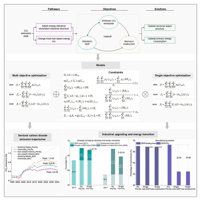
Economic sectors are pivotal in achieving China’s dual carbon goals; nevertheless, the combined impact of industrial and energy consumption structures on sectors’ peak pathways remains unresolved. We extend the optimization of separate industrial and energy structures to a multi-objective dynamic input-output optimization model. Findings indicate the following. (1) China’s energy-related CO₂ emissions are projected to peak in 2028, reaching a volume of 10.06–10.25 Gt. The contribution of industrial structure upgrading to this peak is three times greater than that of energy structure transformation. (2) Approximately 40% of sectors can delay their peaks until after 2030 without impeding China’s overall peaking before 2030. (3) Compared with the single objective of minimizing CO₂ emissions, China can not only achieve its carbon peak earlier but also enhance its average annual gross domestic product (GDP) growth rates by more than 0.26 percentage points and increase the non-fossil energy use’s share by at least 2.78%.

Graphical abstract

Highlights

• •GDP grows by over 0.26 percentage points compared with solely minimizing CO₂
• •40% of sectors may peak after 2030 without impeding China peaking before 2030
• •Pareto-optimal structures better advance industrial upgrades and energy transition
• •Emphasizing industrial upgrading is crucial for China’s carbon peaking efforts

Energy policy; Energy sustainability; Energy systems; Environmental policy

Introduction

China has committed to reaching a CO₂ emission peak by 2030 and achieving carbon neutrality by 2060, known as the “30 · 60” dual carbon goals, in response to global climate change.^1,2,3 In 2021, China’s energy-related CO₂ emissions from economic sectors and residential sources reached 9.67 Gt, excluding process-related emissions. The economic sectors contributed 9.22 Gt CO₂, accounting for 95.43% of the nation’s total energy-related CO₂ emissions.⁴ These sectoral emissions are integral to meeting the ambitious “30 · 60” dual carbon goals. Diverse economic sectors exhibit varying CO₂ emissions due to differences in production processes, technology levels, products, and their roles in the national economy. Notably, in 2021, sectors such as power generation and energy-intensive manufacturing (including sectors of chemicals, non-metallic minerals, and metal smelting) emerged as the primary emission sources, representing 54.35% and 25.60% of total energy-related CO₂ emissions, respectively. Given this scenario, it has become imperative to analyze the future CO₂ emission trajectories of individual sectors. Understanding their peak times and emission volumes is crucial for formulating targeted emission policies. Such policies will facilitate the timely achievement of the dual carbon goals and ensure alignment with the established schedule.

The concept of reaching a peak in CO₂ emissions aims to curb the rate of increase in such emissions. Specifically, altering the composition of economic output and energy consumption mix is crucial for lowering CO₂ emissions through structural adjustments.⁵ Over the past few decades, China’s rise in CO₂ emissions has been propelled by an output structure heavily reliant on energy and a predominant use of coal for energy generation.^6,7 Consequently, it is imperative to overhaul both the output composition and energy consumption structure within China’s economic sectors to attain the desired CO₂ emission peak.^8,9 However, this restructuring effort is not as straightforward as merely reducing emissions from high-intensity sectors (i.e., coal and oil) while boosting low-carbon alternatives (e.g., natural gas and renewable energy). It involves navigating various factors, such as the dynamic input-output balance of economic sectors, production capabilities, and the potential for clean energy adoption. Moreover, as the pursuit of a CO₂ emission peak aligns with sustainable development objectives, other considerations, such as gross domestic product (GDP) growth and employment security, must not be overlooked during the structural adjustment process. Therefore, a comprehensive examination is needed to determine the optimal direction for adjusting output and energy consumption structures across all economic sectors, striking a balance between maximum emission reduction, optimal output levels, and maintaining high employment rates to ensure that China achieves its nationwide CO₂ emission peak target before 2030.

Recently, China’s trajectory toward CO₂ emission reduction has drawn significant attention. Table S1 provides an overview of existing studies examining emission peaks both nationally and across various sectors. At the national level, these studies have primarily focused on China’s emission peak volumes, timings, and trajectories. However, there exists inconsistency regarding the projected peak times. While some researchers suggest that China will peak before 2030,^10,11,12 others argue that the peak might occur after 2030.^13,14,15 This lack of consensus may stem from the inability of national-level analyses to fully capture the nuanced peak strategies required for different economic sectors. Given China’s rapid industrialization and urbanization, economic statuses, production activities, and CO₂ emission characteristics vary significantly.¹⁶ Thus, it is imperative to uncover sector-specific peak strategy requirements to address emissions reduction goals effectively.

At the sectoral level, complex technological and economic interdependencies exist among various economic sectors.¹⁷ Some studies utilized input-output methods to analyze CO₂ emissions.^18,19 However, while this approach effectively delineates inter-industry connections, it falls short in capturing the optimal adjustment direction of inter-sectoral correlations to meet policy objectives such as CO₂ emission peaking targets.²⁰ To address the issue, several studies have proposed optimization models based on input-output tables to identify optimal peaking pathways for economic sectors, considering inter-industry correlations. Currently, two main perspectives dominate this field: single-objective and multi-objective optimization.^21,22

In the realm of single-objective optimization, studies have primarily employed models based on input-output analysis^23,24 and dynamic computable general equilibrium models.^25,26 While these studies account for inter-sectoral relationships, they mainly prioritize a single policy objective, such as maximizing economic benefits or minimizing costs. They do not offer guidance on adjusting inter-sectoral relationships and emission reduction pathways to simultaneously fulfill multiple conflicting policy objectives like economic growth, CO₂ emission reduction, and employment increase while ensuring national CO₂ emission peaking. Although some studies consider multiple policy objectives, they have transformed multi-objective problems into single-objective ones by adopting scalar approaches, such as weighted sum approaches, ε-constraint methods, and goal programming methods.^27,28,29 The utilization of scalar methods can significantly simplify the model-solving difficulty. However, these approaches present difficulties in considering trade-offs between objectives and do not guarantee to find distinct Pareto optimal solutions that represent the Pareto front adequately.³⁰ This can result in the loss of trade-off information among multiple conflicting objectives.³¹

Some studies have attempted to combine multi-objective optimization models with input-output analysis to determine the optimal adjustment direction for either the industrial structure or energy consumption structure separately. However, these studies have fallen short in simultaneously optimizing both the energy consumption mix and industrial structure as decision variables.^32,33 For example, when focusing solely on optimizing the industrial structure, changes in the energy consumption structure are merely a byproduct of the optimized industrial structure.^21,34 Conversely, when solely optimizing the energy consumption structure, accounting for the impact of supply and demand relationships among economic sectors on energy consumption adjustments becomes challenging.³⁵ This limitation may lead to inaccurate estimations of the optimal levels of CO₂ emission reduction potential, value-added growth, and employment increments across economic sectors. Therefore, simultaneous optimization of both the industrial and energy structures is necessary.

To address this research gap, our study explores China’s optimal sectoral CO₂ emission peak pathways by simultaneously optimizing industrial and energy consumption structures at the sectoral level. We accomplish this by developing a CO₂ emission-economy-employment dynamic multi-objective optimization model, which decomposes the national peak target into 28 economic sectors (including service sectors such as traffic services, wholesales, and other services, as listed in Table S2). Our study aims to elucidate how various economic sectors can achieve their CO₂ emission peaks by adjusting sectoral output growth rates and implementing internal energy substitution, all while considering the trade-offs among China’s overall peak target, economic development, and employment growth.

The main contributions of this study are as follows. (1) To address concerns among stakeholders, particularly local governments, regarding the potential impact of achieving a carbon peak on GDP and employment, we have developed a dynamic input-output multi-objective optimization model. This model resolves the challenges encountered by previous studies, which struggled to achieve Pareto optimality in CO₂ emissions, economic output, and employment across all economic sectors in China.^23,25 Our findings indicate that even while striving to reach a carbon peak by 2030, China’s economy and employment can maintain an average annual growth of over 5.3% and 0.5%, respectively. This quantitative evidence updates policymakers’ understanding and helps overcome cognitive barriers, facilitating China’s deeper decarbonization efforts.

(2) Our study overcomes the bottleneck of simultaneously optimizing industrial and energy consumption structures at the sectoral level, achieving Pareto optimal coordination of industrial upgrading, energy transition, and energy security.^21,32 We determine the optimal annual adjustment magnitude for the output of all 28 economic sectors in China and the consumption structure of the four primary types of energy. Additionally, we identify the potential for nurturing strategic emerging industries during the peak-reaching process and the maximum decrease in the ratio of added value in high-carbon, high-energy-consuming industries. Furthermore, we assess the contribution of optimal energy structure adjustments to the stable transition of China’s energy security toward a predominance of non-fossil fuels. These findings offer a systematic and refined basis for decision-making regarding China’s orderly peak in reaching the industry level, accelerating progress toward high-end manufacturing, and providing valuable insights for China’s long-term economic and energy transformation.

Results

The prospective carbon peak trajectories for China

The non-dominated sorting particle swarm optimization (NSPSO) algorithm³⁶ was utilized to solve the proposed dynamic input-output multi-objective model. To evaluate the convergence and uniformity of the algorithm, the center distance ($CD$) and spacing ($SP$) metrics were employed.³⁷ Table S13 presents the statistical information from 50 independent runs using the same data and parameters listed in Table S3. Based on the solution set of the run closest to the average values of $CD$ and $SP$, Figure 1A illustrates 100 groups of Pareto-optimal solutions in the objective space.

Figure 1.

Pareto front and final solutions

(A) 100 groups of Pareto-optimal solutions for multi-objective optimization in low carbon preference (Pre-Lc), economic preference (Pre-Ec), employment preference (Pre-Em), and equality preference (Pre-Eq), and the solutions solely focused on minimizing CO₂ emissions (single min-CO₂), maximizing GDP (single max-GDP), or employment (single max-employment) in the three-dimensional objective space.

(B) Comparison of both CO₂ emission and GDP objectives between Pareto-optimal solution in the equality preference (Pre-Eq) and solution of single min-CO₂.

(C) Comparison of both CO₂ emission and employment objectives between Pareto-optimal solution of Pre-Eq and solution of single min-CO₂.

(D) Comparison of both GDP and employment objectives between Pareto-optimal solution of Pre-Eq and solution of single min-CO₂.

See also Table S13.

To facilitate decision-making, it is crucial to select final solutions from the Pareto solution set. Considering the first three objectives of the model, we establish four types of preferences: low carbon preference (Pre-Lc), economic preference (Pre-Ec), employment preference (Pre-Em), and equality preference (Pre-Eq). Ensuring the dynamic input-output balance constraint of sectors is paramount, making the fourth objective ($f_4$) equally important alongside the priority objective for each preference. Using the multiplicative preference relations method,³⁸ the preference information provided by decision makers is transformed into priority weights ($w_h$) for the objectives, as outlined in Table 1.

Table 1.

Solution sets with different decision preferences

Preferences	Criteria rankinga	Weights $\left(w_1,w_2,w_3,w_4\right)$	$f_1$ (Gt)	$f_2$ (trillion Yuan)	$f_3$ (billion person)
Low carbon preference (Pre-Lc)	$f_4\approx f_1\succ f_2\approx f_3$	(0.499, 0.001, 0.001,0.499)	173.0	2740.7	14.8
Economic preference (Pre-Ec)	$f_4\approx f_2\succ f_1\approx f_3$	(0.001, 0.499, 0.001, 0.499)	173.6	2750.2	14.9
Employment preference (Pre-Em)	$f_4\approx f_3\succ f_1\approx f_2$	(0.001, 0.001, 0.499,0.499)	173.6	2750.2	14.9
Equality preference (Pre-Eq)	$f_4\approx f_1\approx f_2\approx f_3$	(0.250, 0.250, 0.250,0.250)	173.6	2750.2	14.9

Cumulative CO₂ emission (f₁), GDP (f₂), and employment (f₃) from 2018 to 2035 in low carbon preference (Pre-Lc), economic preference (Pre-Ec), employment preference (Pre-Em), and equality preference (Pre-Eq) when the cumulative dynamic input-output balance deviations (f₄) is equally important alongside the priority objective. See also Table S13 and Data S11.

^a$f_1\succ f_2$ represents that $f_1$ is strictly more important than $f_2$, while $f_1\approx f_2$ means that $f_1$ is as important as $f_2$.

The objective values of Pre-Ec are identical to those of Pre-Em and Pre-Eq, indicating undifferentiated results regardless of the ranking of the economic and employment objectives. Employing the multi-criteria tournament decision-gain analysis method (MTD-GAM),³⁹ the solutions for the four preferences in the three-dimensional objective space are delineated in Figure 1.

According to the optimization results, China’s energy-related CO₂ emissions from economic sectors and residents are projected to peak from 2026 to 2030, with a volume ranging from 10.06 to 10.25 Gt (see Figure 2). The most likely year for China’s CO₂ emissions to peak is 2028, occurring with a frequency of 30.5% among 5,000 solutions (see Figure S1), followed by 2029, with a frequency of 25.6%. On average, the CO₂ peak value is estimated to be 10.12 Gt. Compared to developed countries, China—as a developing nation—currently exhibits a high CO₂ emission energy structure and a high energy consumption economic sector structure (see Table S15). The anticipated volume of emissions at the time of reaching its carbon peak is substantial, ranging from 10.06 to 10.25 Gt, with a later peak timing. In contrast, the United States reached its peak at an emission volume of 5.88 Gt, while Japan reached its peak at 1.29 Gt (see Figure S2).

Figure 2.

Energy-related CO₂ emissions trajectory of China (2010–2035)

CO₂ emissions for multi-objective optimization in low carbon preference (Pre-Lc), economic preference (Pre-Ec), employment preference (Pre-Em), and equality preference (Pre-Eq). Emissions for solely minimizing CO₂ emissions (single min-CO₂), maximizing GDP (single max-GDP), or employment (single max-employment).

See also Figures S1–S3; Tables S1, S3, and S15.

Compared to optimization results solely focused on minimizing CO₂ emissions, maximizing GDP, or maximizing employment, the multi-objective Pareto-optimized structures of sectors and energy can facilitate better trade-offs among CO₂ emissions, economic growth, and employment in China as it works toward its carbon peak. After multi-objective optimization, China’s projected carbon peak in 2028 (10.11 Gt) experiences a slight increase of 0.7% compared to the carbon peak in 2025 (10.04 Gt) optimized with the single objective of minimum CO₂ (see Figure 2). However, cumulative GDP and employment can increase by 2.78% and 2.21%, respectively (see Figure 1D). The average annual growth rates could increase by 0.26 and 0.21 percentage points from 2018 to 2030, respectively. This outcome can significantly alleviate concerns among stakeholders, especially local governments, regarding the impact of peaking CO₂ emissions on GDP and employment.

Between 2018 and 2030, sectors reaching their carbon peak (namely power, petroleum, smelting metals, chemicals, and non-metallic minerals) exhibit slightly higher peak carbon volumes under multi-objective optimization compared to single-objective optimization aimed solely at minimizing CO₂ emissions, with an increase of 1.28%–1.73%. Nonetheless, these sectors still achieve their peaks as scheduled (see Figure S3B). However, by 2030, the carbon intensity of these high-carbon sectors under multi-objective optimization could decrease by an additional 0.08% compared to the reduction achieved under single-minimum CO₂ optimization (see Figure S3A).

Furthermore, compared to single-objective optimization, multi-objective optimization significantly enhances China’s CO₂ emissions performance in both industrial and energy structures. From 2018 to 2035, in comparison to optimization results exclusively focused on minimizing CO₂ emissions (single min-CO₂), maximizing GDP (single max-GDP), or employment (single max-employment), the structures achieved through multi-objective optimization (Mo Pre-Eq) achieve reductions in CO₂ emission intensity of 1.68%, 0.08%, and 0.08%, respectively (see Figure 3A). Additionally, per-capita employment-related CO₂ emissions decrease by 1.13%, 0.24%, and 0.24%, respectively (see Figure 3B).

Figure 3.

CO₂ emissions according to GDP and employment in equality preference (Pre-Eq)

(A) Reduction in CO₂ emission intensity by multi-objective optimization (Mo Pre-Eq) compared to single-objective optimization of minimum CO₂ (single min-CO₂), maximum GDP (single max-GDP), or employment (single max-employment).

(B) Reduction in per-capita employment-related CO₂ emissions by multi-objective optimization compared to single-objective optimization of minimum CO₂, maximum GDP, or employment.

See also Figure S3.

Carbon dioxide emission peak paths for economic sectors

Sectoral CO₂ emission trajectories

In contrast to existing studies that solely provide information on the CO₂ emission peak of a nation^10,13 or a single sector,^24,40 this study divides the national economy into 28 distinct economic sectors (see Table S2). Consequently, both the peak times and volumes at the national and sectoral levels can be determined. Using the decision maker’s Pre-Eq as an example, we further analyze all 28 sectors’ CO₂ emission trajectories.

Sectors with CO₂ emission peaks before 2018

Through sectoral output structure and energy mix optimization, the CO₂ emissions of specific sectors peaked before 2018. Among these, the coal mining, textile, and papermaking sectors reached their peaks in 2013 (see Figures 4A and 4B). However, in the business-as-usual (BAU) scenario, CO₂ emissions from the coal mining, textile, and papermaking sectors fail to peak before 2035. Due to strictly constrained targets for coal consumption and renewable energy development, the coal mining sector exhibited the highest peak values of 701.4 Mt in 2012. Conversely, with improvements in energy efficiency, sectors such as gas, wearing, and timber saw their CO₂ emissions peak around 2008 (see Figures 4C and 4D).

Figure 4.

CO₂ emission trajectories for sectors peaking before 2018 in equality preference (Pre-Eq) and business-as-usual (BAU) scenario

(A) CO₂ emission trajectories of the coal mining and petroleum extracting sectors.

(B) CO₂ emission trajectories of the foods, textile, and papermaking sectors.

(C) CO₂ emission trajectories of the gas and nonmetal ores sectors.

(D) CO₂ emission trajectories of the timber, metal mining, and wearing sectors.

See also Figure S4.

Sectors with CO₂ emission peaks in the period (2018–2030)

In decision-making based on the Pre-Eq, five heavy-industry sectors are projected to peak during the period 2018–2030 (see Figures 5A and 5B). The power and petroleum sectors reach peak volumes of 3.5 Gt in 2021 and 2.8 Gt in 2024, respectively (see Figure 5A). The energy consumption structure refers to primary energy sources, including coal, oil, natural gas, and primary electricity. This study’s optimization of the energy consumption structure considers the electrification of end-use energy in the transportation sector and its impact on CO₂ emissions in the power sector.

Figure 5.

CO₂ emission trajectories for sectors peaking in the period 2018–2035 in equality preference (Pre-Eq) and business-as-usual (BAU) scenario

(A) CO₂ emission trajectories of the power and petroleum sectors.

(B) CO₂ emission trajectories of the chemicals, non-metallic minerals, and smelting metals sectors.

(C) CO₂ emission trajectories of the construction sector.

(D) CO₂ emission trajectories of the agriculture and wholesales sectors.

See also Figures S3 and S4, Table S1 and Data S11.

Meanwhile, three energy-intensive manufacturing sectors, namely chemicals (S12), non-metallic minerals (S13), and smelting metals (S14), are expected to reach their CO₂ emission peaks in 2029, 2029, and 2024, respectively (see Figure 5B). The primary reason for this trend is the significant decrease in output shares of these sectors by over 20.0% during the peaking process (see Data S6).

Sectors with CO₂ emission peaks in the period 2031–2035

The agriculture, construction, and wholesales sectors are projected to peak between 2030 and 2035 (see Figures 5C and 5D). Following structural optimizations, agriculture and wholesales sectors are expected to reach their peak CO₂ emissions in 2031 and 2033, respectively, emitting 66.3 Mt and 92.1 Mt (see Figure 5D). The construction sector is also anticipated to reach its peak CO₂ emissions by 2031 (see Figure 5C). Notably, emissions from the construction sector may experience a rapid increase from 2020 to 2031, driven by a 59.84% rise in the sector’s value added (see Data S11). In 2018, the Chinese government explicitly proposed new infrastructure construction projects, particularly in the transportation and power sectors. New infrastructure has emerged as a pivotal driver of China’s economic growth. Although new residential construction may face potential bottlenecks, ample opportunity for urban expansion persists. China’s urbanization rate stood at 66.16% in 2023,⁴¹ indicating significant potential for further growth compared to the approximately 80% level in developed countries.⁴² Renovation of old urban areas and continued infrastructure development will remain key drivers of the sector’s output. Therefore, despite advancements in green building practices, CO₂ emissions from the construction sector are expected to rise.

Sectors without CO₂ emission peaks before 2035

In Pre-Eq decision-making, ten sectors—mainly the high-tech and equipment manufacturing industry sectors (S15–S20), traffic services sector (S26), and other services sector (S28)—are projected to fail to reach their CO₂ emission peaks before 2035 (see Figure 6).

Figure 6.

CO₂ emission trajectories for sectors peaking after 2035 in equality preference (Pre-Eq) and business-as-usual (BAU) scenario

(A) CO₂ emission trajectories of the traffic services and other services sectors.

(B) CO₂ emission trajectories of the general machinery and electrical machinery sectors.

(C) CO₂ emission trajectories of the transport equipment, communication, and other manufacture sectors.

(D) CO₂ emission trajectories of the metal products, measuring instrument, and water sectors.

See also Data S6, S7, S8, S9, and S10.

First, as with per-capita GDP, the demand for transportation in the traffic services sector is expected to keep rising.^43,44 Moreover, hydrogen, particularly green hydrogen derived from renewable sources, holds the potential as a clean energy alternative for China’s transportation industry.^45,46,47 However, challenges persist in hydrogen production, storage, and transportation.^48,49 In essence, decarbonizing transportation comes with significant costs and technical difficulties,⁵⁰ maintaining high pressure for emission reduction within China’s transportation network. Consistent with findings by Chen et al.¹⁴ and Yu et al.,⁴⁰ CO₂ emissions from traffic services are expected to continue rising until 2035 (see Figure 6A).

Second, in line with China’s Outline of the Fourteenth Five-Year Plan for National Economic and Social Development (referred to as the “14th Five-Year Plan”), many high-tech and equipment manufacturing sectors have been identified as strategic emerging industries driving China’s economic growth. These sectors are characterized by their potential for substantial output growth and low-carbon energy consumption structures. From 2017 to the projected peak in 2028, the output share of these strategic emerging industries in China is forecasted to increase from 16.26% to 18.18% (see Data S6). Notably, the coal consumption share in these sectors is expected to decrease significantly, from 10.43% to 3.27%. In comparison, the shares of natural gas and other clean energies are anticipated to rise from 89.57% to 96.73% (see Data S7, S8, S9, and S10). CO₂ emissions from these sectors are projected to continue increasing beyond 2020, with no clear peak expected until 2035 (see Figures 6B–6D). Despite this upward trend in CO₂ emissions, these industries are largely low-emission sectors, contributing less than 5.0% to the total national emissions. Consequently, this trend does not hinder China’s ability to achieve its scheduled carbon peak.

Impact of inter-sectoral carbon dioxide emissions

To assess the influence of changes in one sector’s CO₂ emissions on others, Figures 7 and 8 display direct and indirect CO₂ emissions, respectively. Direct emissions from one sector, driven by activities in other sectors, are the output-induced emissions included in the total output. In contrast, indirect emissions of a sector represent the demand-induced emissions embedded within other sectors. During the process of emission peaking, direct CO₂ emissions are primarily attributed to the petroleum, chemicals, non-metallic minerals, smelting metals, and power sectors (see Figure 7). The notable direct CO₂ emissions from these sectors are driven by the increasing final demand for low-carbon and high-value-added sectors such as construction, high-tech, equipment manufacturing (S16–S19), and other services. Indirect CO₂ emissions from these sectors collectively constitute approximately 80% of the total (see Figure 8).

Figure 7.

Proportion of direct sectoral CO₂ emissions driven by other sectors

Direct CO₂ emissions in 2017, peak years (2027 in low carbon preference (Pre-Lc) and 2028 in equality preference (Pre-Eq)), and 2035.

See also Figures S3 and S4.

Figure 8.

Share of indirect CO₂ emissions induced by sector

(A) Share of indirect CO₂ emissions by sector in the low carbon preference (Pre-Lc).

(B) Share of indirect CO₂ emissions by sector in the equality preference (Pre-Eq).

See also Figure S4.

With the widespread adoption of green building standards, the portion of indirect CO₂ emissions stemming from construction is projected to gradually decline from 39.2% in 2017 to approximately 33.0% by 2027 or 2028 (see Figure 8). However, the shares of indirect emissions from the high-tech and equipment manufacturing sectors (S16–S19) and other services exhibit upward trajectories. Notably, the high-tech and equipment manufacturing sectors (S16–S19) can experience the most substantial growth rates, rising from 17.9% in 2017 to 28.6% (Pre-Eq) or 29.0% (Pre-Lc) by the peak year. This trend may be attributed to the structural shift toward digital, intelligent, and green development in the economy, resulting in rapid investments in strategic emerging industries.

Changes in sectoral output structure, energy consumption mix, and employment

Structural changes in sectoral output

Between 2017 and the peak years (2027 in Pre-Lc and 2028 in Pre-Eq), the output proportions of the agricultural and heavy-industry sectors undergo varying degrees of decline following economic restructuring. As depicted in Figure 9, the output shares of power (S22) and petroleum (S11) experience the most pronounced decreases, plummeting by over 43.0% (Pre-Lc) and 47.0% (Pre-Eq), respectively. Conversely, sectors witnessing output proportion increases are predominantly the high-tech and equipment manufacturing sectors (S16–S20) and other services sectors (S28). Notably, the measuring instrument sector (S20) exhibits the most substantial output growth, reaching 35.0% (Pre-Lc) and 37.0% (Pre-Eq).

Figure 9.

Structural changes in sectoral output from 2017 to the peak year

Change of output shares for different economic sectors in the low carbon preference (Pre-Lc) and equality preference (Pre-Eq).

See also Data S6.

These shifts are primarily influenced by China’s industrial policy aimed at “reducing overcapacity and adjusting its economic structure.” Leading up to the peak years, the expansion of output in the petroleum and power sectors is managed to some extent, with an annual average growth rate of less than 1.2%. In contrast, the measuring instrument sector is expected to maintain a growth rate of approximately 10.0%, supported by policies promoting the development of strategic emerging industries.

Energy consumption mix changes in the peaking process

Even after adjusting the energy structure, China’s energy consumption mix remains predominantly fossil-based, constituting over 60% of primary energy (see Figure 10). Fossil energy is projected to peak in 2030, reaching a volume of 4.4 billion ton of standard coal equivalent (tce). Coal consumption peaked in 2014, while oil consumption peaked in 2021 (Pre-Lc) and 2022 (Pre-Eq). The shares of natural gas and non-fossil energy consumption are anticipated to witness significant growth, rising from 6.9% and 13.6% in 2017 to over 15.0% and 25.0% by 2030, respectively. Two key factors drive this transition to a low-carbon energy structure. First, China is poised to rigorously control fossil fuel consumption over the next decade, progressively reducing coal usage, increasing electric vehicle adoption, and curbing oil consumption. Second, bolstered by renewable energy policies and advancements in power generation technologies, carbon-free energy sources such as hydropower, wind power, and solar photovoltaics have experienced rapid development, effectively substituting fossil fuels.

Figure 10.

China’s energy consumption (1995–2035)

(A) China’s energy consumption in the low carbon preference (Pre-Lc).

(B) China’s energy consumption in the equality preference (Pre-Eq).

See also Data S7, S8, S9, and S10.

In contrast to the national-level energy structure optimization conducted by Yu et al.,⁵¹ this study focuses on optimizing the internal energy structure within individual sectors, considering sectoral input-output correlations. Based on the contribution of sectoral CO₂ emissions (see Figure S4), nine key sectors significantly influence changes in CO₂ emissions before and after the peak. These sectors include power (S22), petroleum (S11), energy-intensive sectors (S12–S14), construction (S25), and tertiary industry sectors (S26–S28). Figure 11 illustrates the changes in energy consumption structures, specifically within these nine sectors, from 2017 to the peak year.

Figure 11.

Changes in sectoral energy structure in the equality preference (Pre-Eq)

(A–I) Represents the energy structure changes in power, petroleum, energy-intensive manufacturing sectors, construction, and the tertiary industry sectors, respectively.

See also Figure S4, Table S2, Data S7, S8, S9, and S10.

Throughout the peak process, notable shifts occur in the energy structures of both heavy and tertiary industry sectors. Using Pre-Eq as an example, the tertiary industry sectors (S26–S28) markedly decrease their reliance on fossil fuel energy by over 14.0% (see Figures 11G–11I). Consequently, the proportion of non-fossil energy consumption surges by approximately 60.0% in the non-metallic minerals sector (see Figure 11D), followed by the chemicals sector (over 30%) (see Figure 11C) and traffic services sector (more than 40.0%) (see Figure 11G).

Structural changes in sectoral employment

During the process of achieving the CO₂ emission peak, the total employment figures exhibit a steady increase, rising from 776.4 million persons in 2017 to 869.2–872.1 million persons by 2035 in China. As industrial structure adjustments unfold, there is a notable shift of employees from high-carbon to low-carbon sectors. As outlined in Table 2, the employment rate within the tertiary industry sectors (S26–S28) is projected to reach 51.6%–53.3%, assuming a pivotal role in ensuring future employment security. The high-tech and equipment manufacturing sectors (S15–S20) are expected to witness the most substantial growth from 2017 to the peak year, with an increase of 37.5%–41.2%, emerging as the second preferred destination for labor transferred from other industry sectors. In contrast, the share of employment within the agriculture and energy-intensive manufacturing sectors (S12–S14) is anticipated to decline sharply, followed by the consumer goods manufacturing sectors (S6–S10).

Table 2.

Changes in employment shares by sector (unit: %)

Sectors(code)	2017	Pre-Lc		Pre-Eq
		Peak year (2027)	2035	Peak year (2028)	2035
Other Services (S28)	30.5	34.2	36.5	36.0	39.1
Agriculture (S1)	27.0	15.9	9.9	14.7	9.5
Wholesales (S27)	11.4	13.2	15.5	13.1	14.8
Construction (S25)	8.9	11.3	13.2	11.8	13.6
High-tech and equipment manufacturing (S15–S20)	7.4	10.4	11.4	10.1	10.6
Consumer goods manufacturing (S6–S10)	5.6	4.7	4.0	4.5	3.7
Energy-intensive manufacturing (S12–S14)	4.1	3.4	1.4	3.1	1.4
Traffic Services (S26)	3.0	4.2	5.5	4.1	5.1
Other sectors (S2–S5, S11, S21–S24)	2.2	2.6	2.4	2.5	2.3

Employment shares by sector. Change of employment shares for other services, agriculture, wholesales, construction, high-tech and equipment manufacturing, consumer goods manufacturing, energy-intensive manufacturing, traffic services, and other sectors before and after the peak in low carbon preference (Pre-Lc) and equality preference (Pre-Eq). See also Tables S2 and S9.

Uncertainty analysis

The multi-objective optimization model in this study comprises three types of parameters. The first category includes basic technical and economic parameters, such as the CO₂ emission coefficient $p_k$ and the maximum exploitable technological potential of non-fossil energy $E{P}_t$. The second category involves the government’s plan or target parameters, including the maximum primary energy consumption $T{E}_t$ in key years and the shares of different primary energy consumption ${\lambda }_t$ and ${\mu }_{kt}$. The last category contains the estimated parameters based on historical data, including the minimum annual growth rate of GDP $r_t$ and the growth rates of energy intensity ${\beta }_1$ and ${\beta }_2$. The first two parameter types are relatively stable; however, the latter has more uncertainty. Hence, the results of this study may be affected more by the uncertainty in the third parameter. Therefore, the sensitivity of the model’s main uncertainty parameters is analyzed to assess the robustness of the parameter sets and the reliability of the optimization results.

Minimal annual GDP growth rate

As a major developing country, to achieve the second “Centenary Goal,” China needs to maintain a growth rate of 5.0%–6.0% before 2030.⁵² According to recent data, the average GDP growth rate from 2021 to 2023 reached 5.5%.⁵³ Yu et al.⁵⁴ and Lu et al.⁵⁵ have set China’s minimum GDP growth rate above 5.0% until 2030. Thus, the baseline scenario of minimal annual GDP growth rates (R₀) is set at 5.5% for 2021–2025 and 5.0% for 2026–2030, respectively (see Table S10). Based on the baseline settings, the low GDP growth scenario (R_L) and high GDP growth scenario (R_H) are set up by decreasing and increasing by 0.5 percentage points, respectively.

Minimum annual energy intensity improvement rate (${\beta }_2$)

The baseline scenario of energy intensity improvement is 1.67% per year (scenario EI₀) and minimum annual energy intensity improvement rate (${\beta }_2$) is 0.7. The energy intensity improves by 2.0% (${\beta }_2=0.64$) and 1.11% (${\beta }_2=0.8$) per year in the faster improvement scenario (scenario (EI_H) and lower improvement scenario (scenario EI_L), respectively, which refer to the relevant settings.^51,56

After analyzing the parameter settings, we found that China’s peak time and volume of CO₂ emissions are significantly influenced by the minimum annual GDP growth rate and energy intensity improvement (see Figure 12). Under a low GDP growth scenario (R_L), the peak of CO₂ emissions is expected in 2026 (frequency: 42.2%), with a volume ranging from 10.00 to 10.18 Gt. Conversely, under a high GDP growth scenario (R_H), the peak is projected around 2030 (frequency: 46.7%), with a volume between 10.19 and 10.30 Gt, approximately 1.3% higher than the baseline scenario (BL₀) (see Figure 12B). In the scenario with faster energy efficiency improvement (EI_L), the CO₂ emission peak is likely to occur by 2025 (frequency: 72.8%), with volumes ranging from 10.04 to 10.14 Gt. Conversely, in the slower energy efficiency improvement scenario (EI_H), the peak is anticipated around 2030, with a range of 10.15–10.31 Gt, nearly 0.9% higher than the baseline scenario (see Figure 12C).

Figure 12.

Sensitivity analysis results for China’s overall carbon dioxide emissions

(A) Peak time, peak volume, and the most likely peak time in the baseline scenario (BL₀) with minimal annual GDP growth rates (R₀), minimum annual energy intensity improvement rate (EI₀).

(B) Peak time, peak volume, and the most likely peak time in a low GDP growth scenario (R_L) and a high GDP growth scenario (R_H).

(C) Peak time, peak volume, and the most likely peak time in the faster energy efficiency improvement scenario (EI_L) and lower energy efficiency improvement scenario (EI_H).

See also Table S10.

In essence, reducing the minimum GDP growth rate by 0.5 percentage points and improving energy efficiency by 0.3 percentage points annually compared to the baseline scenario results in an emission peak three years earlier under the low GDP growth scenario compared to the high GDP growth scenario, with a peak volume reduced by approximately 1.0%.

At the sectoral level, we focused on sectors peaking between 2018 and 2035 to analyze changes in peak time and volume (see Figure 13). Notably, the petroleum, power, and energy-intensive manufacturing sectors (S12–S14) exhibit the highest sensitivity to peak times. When the minimum annual GDP growth rate is adjusted by ±0.5 percentage points, sectors including petroleum, power, chemicals, and non-metallic minerals experience shifts in CO₂ emission peaks ranging from one to six years earlier or one to five years later (see Figures 13A–13D). Similarly, when the minimum annual growth rate of energy intensity improvement is increased by 0.3 or reduced by 0.5 percentage points per year, sectors such as petroleum, power, and smelting metals reach their emission peaks two to five years earlier or delay peaking by four to six years. Conversely, under scenarios of slowed GDP growth and sharp improvements in energy intensity, sectors such as agriculture and wholesales may experience delayed peak times and increased peak volumes (see Figures 13P and 13R). This dynamic arises from the significant contribution of petroleum, power, and energy-intensive manufacturing sectors (S12–S14) to China’s CO₂ emissions. To expedite the peak of CO₂ emissions, growth rates in these sectors need to be constrained. In contrast, tertiary industry sectors, characterized by low CO₂ emissions and high value-added features, can be developed to ensure stable economic growth.

Figure 13.

Sensitivity analysis results of sectoral carbon dioxide emissions

(A–I) Changes of peak time in the sectors peaking between 2018 and 2035 under the baseline scenario (BL₀), the low GDP growth scenario (R_L) and high GDP growth scenario (R_H) and the faster energy efficiency improvement scenario (EI_L) and lower energy efficiency improvement scenario (EI_H), respectively.

(J–R) Changes of peak volume in these sectors under the baseline scenario (BL₀), the low and high GDP growth scenario (R_L and R_H), the faster and lower energy efficiency improvement scenario (EI_L and EI_H), respectively.

See also Table S10.

Discussion

Multi-objective optimized structure contributes to industrial upgrading and energy transition

Multi-objective optimization of industrial structure, compared to single-objective optimization, significantly contributes to China’s industrial upgrading. From 2017 to 2030, after multi-objective optimization, the value-added and employment shares of strategic emerging industries (S15–S20) and the tertiary industry (S26–S28) increase from 61.86% and 52.28% to 70.05% and 69.55%, respectively (see Figure 14A). Conversely, the GDP and employment shares of the energy conversion sectors (S11 and S22) and the energy-intensive sectors (S12–S14) decrease from 12.33% and 4.80% to 8.83% and 1.84%, respectively (see Figure 14B). Multi-objective trade-off optimization, in contrast to optimization solely aimed at minimizing CO₂ emissions, reveals additional value-added potential of 1.88% and 0.43% in sectors, along with increased employment potential of 9.90% and 27.04%. These optimized outcomes imply significant industrial upgrades in China.

Figure 14.

Comparison of the contribution of multi-objective and single-objective optimization to industrial upgrading and energy transformation

(A) Growth in the value-added and employment shares of strategic emerging industries and the tertiary industry after multi-objective optimization, compared to single-objective optimization.

(B) Reduction in the value-added and employment shares of energy conversion sectors and energy-intensive sectors after multi-objective optimization.

(C) Enhancements in GDP per employment and CO₂ emission efficiency (GDP created per unit of CO₂ emissions) in the manufacturing sector.

(D) Additional low-carbon energy potentials from Pareto optimal energy consumption structure.

See also Data S7, S8, S9, S10, and S11.

Furthermore, multi-objective industrial structure optimization leads to enhancements in GDP per employment and CO₂ emission efficiency (GDP created per unit of CO₂ emissions) in the manufacturing sector (S6–S20) by 65.10% and 66.19%, respectively (see Figure 14C). Compared to optimization targeting solely GDP or employment maximization, these results unlock more than 0.65% and 23.89% additional potential for labor output efficiency and CO₂ emissions efficiency improvement, respectively. This highlights that the Pareto-optimal structure achieved through multi-objective trade-offs better advances China’s manufacturing industry toward higher levels.

Multi-objective optimization proves more effective in facilitating China’s energy transition than single-objective optimization. Results from structural multi-objective optimization indicate that from 2017 to 2030, the share of non-fossil energy consumption in China is projected to rise from 13.60% to 25.74%, while coal consumption is expected to decline from 60.60% to 43.58% and crude oil consumption from 18.90% to 14.74% (see Figure 14D). Compared to optimization solely focused on maximizing GDP or employment, multi-objective trade-off Pareto optimization reveals additional low-carbon energy potentials of at least 2.78%, 0.76%, and 5.09%. This underscores the effectiveness of multi-objective optimization in aligning with China’s planned target for a non-fossil energy consumption structure (25%) and advancing energy transition efforts.

Contribution of collaborative multi-objective optimization of industrial and energy structures to the carbon peak of China and its economic sectors

The contribution of industrial structure upgrading to China’s timely achievement of its carbon peak exceeds that of the low-carbon transition of energy structures by more than 3-fold. After multi-objective optimization from 2017 to the peak year (2028), industrial structure upgrading contributes 456.3% to China’s carbon peak, whereas the contribution from the low-carbon transition of energy structures is 143.2% (see Figure 15A). Furthermore, the gap between their contributions widens progressively (see Figure 15B).

Figure 15.

Decomposition of CO₂ emission-driving factors before and after the peak

(A) Contribution to emission reductions from changes in the GDP, industrial structure (IS), energy intensity (EI), energy consumption structure (ES), and CO₂ emission coefficient (EC).

(B) Contribution to emission reductions from changes in the industrial structure and energy consumption structure by year.

See also Table S14.

Regarding the higher contribution of industrial restructuring to China’s carbon reduction compared to energy structure transformation, two primary reasons can be identified. Firstly, despite the inherent challenges associated with industrial restructuring, particularly considering technological advancements and potential market demand, China has made significant progress in its low-carbon transformation of industrial structures. The output value of energy-intensive and carbon-intensive sectors such as cement, iron and steel and building materials has significantly contracted as traditional infrastructure projects near completion.⁵⁷ Concurrently, the output value of strategic emerging industries has rapidly increased, with the value-added contribution of these industries to China’s GDP exceeding 13% in 2022.⁵⁸ This industrial upgrading has unlocked substantial potential for carbon emission reduction. Specifically, changes in industrial structure reduced carbon emissions by 153.19 million tonnes from 2007 to 2016⁵⁷ and by 260.99 million tonnes from 2017 to 2018.⁵⁹

Secondly, constrained by its energy resource endowment, China relies heavily on coal to ensure a secure energy supply. It is challenging to significantly reduce the proportion of coal consumption within a short time frame.⁶⁰ Even by the anticipated carbon peak year of 2028, coal consumption in China is expected to remain around 46%, significantly higher than the levels in developed countries such as the USA (11.4%) and the UK (2.9%) in 2021. Consequently, in the short term, the transition in China’s energy structure will have a limited impact on CO₂ emissions reduction.^61,62

From a sectoral perspective (see Table S14), the contribution to emission reductions from changes in the energy structure within the consumer goods manufacturing sectors (S6-S10) and the wholesales sectors (S27) (1361.81%) is significantly higher than that resulting from changes in their outputs due to industrial restructuring (691.35%). Furthermore, industrial upgrading plays a significant role in achieving carbon peaks in the energy conversion sector (S11 and S22) and energy-intensive sectors (S12–S14).

Conclusion

To ensure China meets its carbon peak target, this study proposes optimizing industrial and energy structures simultaneously in a multi-objective optimization model. This approach aims to achieve balanced and orderly emission peaks across economic sectors by dynamically considering input-output balance constraints. By redesigning emission peak pathways through optimal adjustments to industrial and energy structures, the following conclusions emerge.

• 1)Approximately 40% of China’s economic sectors can peak after 2030 while maintaining specific GDP growth rates (e.g., not less than 5.0% during 2025–2030) and increasing employment. These sectors include low-carbon, high-value-added service industries and strategic emerging sectors. This adjustment does not hinder China from reaching its national CO₂ emission peak target ahead of schedule. This is attributed to emission-intensive sectors like power, petroleum, and three energy-intensive manufacturing sectors (S12–S14) being primary CO₂ emission sources in China, which will peak earlier than 2030 with optimized industrial and energy structures.
• 2)The results from our proposed multi-objective model offer significant advantages for China in achieving its scheduled carbon peak by balancing economic growth and boosting employment compared to single-objective optimization approaches. By integrating multiple objectives, our model enhances China’s CO₂ emission performance. Compared to three single-objective optimization approaches (minimizing CO₂ emissions, maximizing GDP, and maximizing employment), our multi-objective optimization yields notable improvements. From 2018 to 2030, average annual GDP and employment growth rates increase by 0.26 and 0.21 percentage points, respectively. Moreover, per-capita employment CO₂ emissions and carbon intensity decrease by 0.35%–1.18% and 0.10%–0.85%, respectively. Specifically, the strategic emerging and tertiary industry sectors see significant gains, with added value and employment shares increasing by 1.88% and 9.90%, respectively. Conversely, the proportion of added value from low value-added, high-carbon, and high-energy-consuming sectors drops by 0.43%. Additionally, non-fossil energy consumption rises by 2.78%, while coal and crude oil consumption declines by 0.76% and 5.09%, respectively.
• 3)Upgrading sectoral output structures emerge as crucial for achieving carbon peaks in China, highlighting the need to avoid overreliance on energy structure adjustments for CO₂ emission reduction. Following multi-objective optimization, the contribution of industrial structure upgrading to China’s carbon peak reaches 456.3%, surpassing the 143.2% contribution from low-carbon energy structure transformation. Notably, low-carbon energy structure transformation plays a pivotal role in carbon peaking for consumer goods manufacturing sectors (S6–S10) and wholesales sectors (S27). Conversely, adjusting output structures is vital to carbon peaking in high-carbon and high-energy-consuming economic sectors (S11–S14 and S22).

The potential impact of this study is as follows. We address the concerns of local governments and companies regarding the impact of carbon peaking on GDP and employment in China. We demonstrate that achieving a carbon peak ahead of schedule is feasible while maintaining robust average annual GDP and employment growth rates of over 5.3% and 0.5%, respectively. By employing multi-objective optimization, our study provides clarity on the annual optimal adjustment range for output and primary energy structures across all sectors in China. These findings serve as a valuable decision-making tool for promoting industrial upgrades and low-carbon energy transformation in the country.

The directions for future work are as follows. This study’s framework, based on dynamic input-output multi-objective modeling, holds promise for addressing similar challenges in energy, environmental, and economic systems beyond carbon peaking. Future research avenues include exploring technical pathways for achieving carbon neutrality in economic sectors considering conflicting objectives such as cost, benefit, and CO₂ emission reduction. Additionally, there is potential to investigate the orderly development of renewable energy at regional levels, offering insights into sustainable energy transitions and environmental stewardship.

Based on the findings of this study, we suggest the following policy implications. First, to further advance the decrease in national peak volume while ensuring the timely carbon peak, the Chinese government should prioritize attention to five key sectors: power, petroleum, chemicals, non-metallic minerals, and smelting metals. These sectors are projected to achieve carbon peaks between 2021 and 2029.

Second, to safeguard energy supply security, China must annually decrease the proportion of fossil energy consumption during the carbon peak period. Specifically, from 2017 to the peak year (2028), coal consumption should decrease by a minimum of 2.4% annually, oil consumption by over 1.8% annually, and non-fossil energy consumption should increase by an average of 5.2% annually. Within the manufacturing sector, coal consumption should be reduced by 0.04% annually, while non-fossil energy consumption should increase by 5.5% annually.

Third, to meet the policy objective of “ensuring employment for residents,” the Chinese government should prioritize tertiary industry sectors and high-tech and equipment manufacturing sectors (S15–S20). By the peak year, the employment rate in tertiary industry sectors (S26–S28) should surpass 50.0%. High-tech and equipment manufacturing sectors (S15–S20) should sustain an increase of over 37.0% from 2017 to the peak year. Nationally, these sectors represent the future employment landscape, necessitating urgent attention from the Chinese government to enhance talent cultivation and reserves.

Limitations of the study

This study has two limitations. First, the national economy is aggregated into 28 economic sectors. Obtaining more detailed data, such as energy consumption data for the subsectors of the tertiary industry, could enable a more refined delineation of sectors within the tertiary industry. This, in turn, would facilitate the design of more precise peaking pathways. Second, the utilization rate of clean energy is significantly influenced by the usage cost of renewable energy.^63,64 Future research could explore the impact of varying renewable energy usage costs on energy structure adjustments, provided that the necessary data are available.

STAR★Methods

Key resources table

REAGENT or RESOURCE	SOURCE	IDENTIFIER
Deposited data
Input-output tables of China for 2012 and 2017	National Bureau of Statistics of China	https://data.stats.gov.cn/
GDP, sectoral value-added, and power generation installed capacity	China Statistical Yearbook for 2020	https://data.stats.gov.cn/
sectoral employees	China Economic Census Yearbooks and China Population Census Yearbook	https://data.stats.gov.cn/
Sectoral primary energy consumption	China Energy Statistical Yearbooks from 2009 to 2019	https://www.nea.gov.cn/
Data generated by this study (optimal sectoral output, energy consumption, value-added)	This study (supplemental information)	Data S6, S7, S8, S9, S10, and S11
Software and algorithms
MATLAB R2020b	MathWorks	https://www.mathworks.com/products/matlab.html
Origin 2017	OriginLab	https://www.originlab.com/OriginProLearning.aspx
NSPSO, MTD-GAM	This study (supplemental information)

Resource availability

Lead contact

Further information and requests for resources and reagents should be directed to and will be fulfilled by the lead contact, Shiwei Yu (yusw@cug.edu.cn or ysw81993@sina.com).

Materials availability

This study did not generate new unique materials.

Data and code availability

• •This study analyzes existing, publicly available data, which are listed in the key resources table. The data generated by our analysis can be found in Data S6, S7, S8, S9, S10, and S11.
• •The code for the analysis was written in MATLAB and is available in this paper’s supplemental information.
• •Any additional information required to reanalyze the data reported in this study is available from the lead contact upon request.

Method details

CO₂ emission-economic-employment multi-objective optimization model

The framework of the proposed model

Different economic sectors exhibit varying technological and production process levels, resulting in significant differences in energy consumption even with similar sectoral output. Thus, efficient restructuring of a country’s economic output can achieve peak CO₂ emissions without diminishing total output.⁶⁵ The energy consumption of a sector is typically correlated with the goods or services it produces. Consequently, restructuring sector output often entails changes in the energy structure. Primary energy sources possess different carbon contents per unit calorific value, leading to variations in unit CO₂ emissions. Therefore, CO₂ emissions can be mitigated by adjusting the energy consumption structure without reducing total consumption.⁵¹

Adjusting the economic structure and energy mix represents fundamental measures for achieving sustainable development. While economic development remains the primary target of structural adjustments, safeguarding the environment and mitigating the adverse effects of CO₂ emissions on human survival and economic development are equally important objectives. However, economic development may exacerbate CO₂ emissions if carbon-intensive sectors contribute significantly to GDP. Restricting the output of carbon-intensive sectors could reduce emissions but might impede economic growth.²² Thus, economic development and CO₂ emissions reduction present conflicting objectives. Sustaining high levels of employment in China is paramount for facilitating structural transformation and ensuring social stability.³⁶ Industrial and energy structure adjustments constitute multi-objective optimization challenges.

Furthermore, restructuring output and energy consumption entails not only reducing emissions from intensive sectors and decreasing the share of fossil fuel consumption but also increasing output from low-carbon sectors and renewable energy sources, respectively. This adjustment process is influenced by factors such as the input-output balance among sectors and each sector’s production capacity. Failure to consider these factors can lead to structural economic imbalances and uncertainty, potentially harming economic development. Therefore, maintaining an input-output balance is crucial for the scientific development of a multi-objective optimization model for industrial and energy consumption structures.

Additionally, macro policies like industrial and energy structure adjustments often have enduring effects on socioeconomic environments. To measure the long-term effects of changes in industrial and energy consumption structures on CO₂ emission trajectories across different economic sectors, it is necessary to consider the dynamic input-output relationships among sectors.^66,67 This dynamic input-output balance serves as a critical constraint for achieving dynamic adjustments in economic structure.

Hence, we propose a CO₂ emission-economic-employment multi-objective model that integrates a dynamic input-output model with multi-objective optimization to analyze CO₂ emission peak pathways at the sectoral level. The framework of this proposed model is depicted in Figure S5.

Model assumptions

This study investigates the achievement of energy-related CO₂ emission peaks through structural optimization across the entire industrial sector. Given that the optimization process encompasses the energy consumption processes of all economic sectors, we propose the following three assumptions:

• 1)Basic assumptions of the input-output model: We adhere to the “pure” sector (homogeneity) assumption, wherein each industrial sector produces only one specific homogeneous product with constant returns to scale.
• 2)We solely consider CO₂ emissions from fossil fuel combustion, excluding process-related emissions such as those from cement production.
• 3)Exogenous technological progress: The direct consumption coefficient $A_t$ in the period from 2018 to 2035 is updated using the RAS method based on the Chinese input-output tables for 2012 and 2017.⁶⁸

Basic linear equations of the Leontief dynamic model

The static input-output model offers insights into the state of the economic system at a specific point in the past. However, industrial and energy restructuring aims to understand how changes in sectoral output and energy consumption influence future CO₂ emissions and economic growth, emphasizing the dynamic nature of adjustments.

The dynamic input-output model, an economic dynamic model, focuses on studying structural changes in economic sectors.⁶⁹ This model examines the quantity and internal relationship between capital investment in the previous period and sectoral output in the subsequent period. Dynamic models, including the dynamic input-output model, have found widespread application in carbon-related studies.^40,66

Given the dynamic nature of structural adjustment, this study employs the Leontief dynamic model⁷⁰ to investigate the repercussions of changes in sectoral output and energy consumption on the economy, energy, and environment from year $t$ to year $t+1$. The fundamental linear equations of the Leontief dynamic model are outlined as follows:

$$\left(I-A_t\right)X_t=Q_t\left(X_{t+1}-X_t\right)+{\tilde{F}}_t$$ (Equation 1)

$$\left(I-A_{ct}\right)X_t=G_t$$ (Equation 2)

Suppose there are $N$ sectors in the economy. $X_t={\left({\left(x_1\right)}_t,{\left(x_2\right)}_t,\cdots ,{\left(x_N\right)}_t\right)}^T$ is the total output vector in year $t$ with $N$ dimensions, where ${\left(x_j\right)}_t$ is the output of sector $j$. $X_t$ is a decision variable in the model, and $X_t\ge 0$. $A_t={\left({\left(a_{ij}\right)}_t\right)}_{N\times N}$ is the direct consumption coefficient matrix for year $t$ with $N\times N$ dimensions, where $a_{ij}$ denotes the direct consumption of sector $i$ per unit output of sector $j$. $I$ is the identity matrix with $N\times N$ dimensions. $\left(I-A_t\right)X_t$ refers to the final product or output. $Q_t={\left({\left(q_{ij}\right)}_t\right)}_{N\times N}$ is the investment coefficient matrix in year $t$ with $N\times N$ dimensions, where $q_{ij}$ represents the investment products of sector $i$ required per unit output of sector $j$.

$Q_t\left(X_{t+1}-X_t\right)$ is the capital formation vector in year $t$,namely the newly added capital in year $t$, which is used to expand the output scale ($\Delta X=X_{t+1}-X_t$) in year $t+1$. Capital formation connects the change in a sector’s output in year $t+1$ to the required capital investment in year $t$, reflecting the impact of sectoral output changes in year $t+1$ on capital formation in year $t$.

${\tilde{F}}_t$ is the final net product vector in year $t$ with $N$ dimensions. The sum of capital formation $Q_t\left(X_{t+1}-X_t\right)$ and the final net product ${\tilde{F}}_t$ is the final demand. $A_{ct}=\text{diag}\left[\sum _{i=1}^N{\left(a_{i1}\right)}_t,\sum _{i=1}^N{\left(a_{i2}\right)}_t,\cdots ,\sum _{i=1}^N{\left(a_{iN}\right)}_t\right]$ is a diagonal matrix of the intermediate input ratio with $N\times N$ dimensions. $\left(I-A_{ct}\right)X_t$ denotes the initial input vector for year $t$. $G_t={\left({\left(g_1\right)}_t,{\left(g_2\right)}_{t,\cdots ,}{\left(g_N\right)}_t\right)}^T$ is the value-added vector in year $t$ with $N$ dimensions, where ${\left(g_j\right)}_t=\left(1-\sum _{i=1}^N{\left(a_{ij}\right)}_t\right){\left(x_j\right)}_t$ is the added value of sector $j$.

Objective functions

• a)Minimum sectoral carbon dioxide emissions

In the context of addressing climate change, attaining a CO₂ emissions peak by 2030 represents a crucial milestone for China in its pursuit of carbon neutrality by 2060. Given that CO₂ emissions primarily stem from the production activities of economic sectors, these sectors wield significant influence over emissions control. Consequently, setting the minimum cumulative value of sectoral CO₂ emissions as the primary objective is imperative.

$$\min f_1=\sum _{t=1}^M\sum _{j=1}^N\sum _{k=1}^K{p}_k{\left(y_{jk}\right)}_t$$ (Equation 3)

where $Y_t={\left({\left(y_{jk}\right)}_t\right)}_{N\times K}$ is the primary energy consumption matrix for different economic sectors in year $t$ with $N\times K$ dimensions, and ${\left(y_{jk}\right)}_t$ is the consumption of energy $k$ in sector $j$ ($k=1,2,3,4$ refers to coal, oil, natural gas, and non-fossil energy, respectively). $Y_t$ is another decision variable in the model and $Y_t\ge 0$. $p_k$ denotes CO₂ emissions per unit of energy consumption $k$, which is an exogenous parameter. $p_k{\left(y_{jk}\right)}_t$ represents the CO₂ emissions from energy $k$ from sector $j$ in year $t$. $M$ represents the number of years in the planning period. $N$ represents the number of economic sectors. $K$ represents the number of primary energy types.

Residents' energy consumption is treated as an exogenous variable because it only accounted for 4.57% of total energy-related CO₂ emissions in 2021.⁴ The growth potential for direct CO₂ emissions from residents is limited, as their energy consumption is expected to be primarily dominated by electricity. Furthermore, residential energy consumption is anticipated to increase steadily, driven by China's urbanization and improving living standards.

• b)Maximum GDP

As a developing country, it is unrealistic for China to reduce its GDP significantly to achieve the CO₂ emission peak. The promotion of industrialization and urbanization requires a solid economic basis. Therefore, maximizing the cumulative value of China’s GDP is an essential goal.

$$\max f_2=\sum _{t=1}^M\sum _{j=1}^N\left({1-\left(a_{·j}\right)}_t\right){\left(x_j\right)}_t$$ (Equation 4)

where ${\left(x_j\right)}_t$ is the output of sector $j$ for year $t$. ${\left(x_j\right)}_t$ is a decision variable in the model and ${\left(x_j\right)}_t\ge 0$. ${\left(a_{·j}\right)}_t=\sum _{i=1}^N{\left(a_{ij}\right)}_t$ represents the intermediate input per unit output of sector $j$ for year $t$. $\left({1-\left(a_{·j}\right)}_t\right){\left(x_j\right)}_t={\left(g_j\right)}_t$ denotes the value-added of sector $j$ in year $t$. $\sum _{j=1}^N\left({1-\left(a_{·j}\right)}_t\right){\left(x_j\right)}_t$ is the GDP in year $t$. The GDP is calculated according to the production method.

• c)Maximum employment

During structural adjustment, labor- and carbon-intensive sectors might experience reduced job demands due to constraints on output growth. Conversely, low-carbon and high value-added sectors may witness increased employment opportunities as production capacity expands. Facilitating inter-sectoral labor shifts from labor- and carbon-intensive sectors to low-carbon and high value-added sectors holds significant importance in sustaining employment stability and social security. Thus, maximizing the cumulative value of employment is established as the third objective.

$$\max f_3=\sum _{t=1}^M\sum _{j=1}^N{\left(l_j\right)}_t\left({1-\left(a_{·j}\right)}_t\right){\left(x_j\right)}_t$$ (Equation 5)

where ${\left(l_j\right)}_t$ is the workforce required per unit value added of sector $j$ in year $t$, which is an exogenous parameter. ${\left(l_j\right)}_t\left({1-\left(a_{·j}\right)}_t\right){\left(x_j\right)}_t$ is the workforce of sector $j$ in year $t$.

Constraints

Economic sector linkage constraints

• a)Sectors’ dynamic input-output balance

In the broader economic system, distinct input and output linkages exist among various industrial sectors. Maintaining a supply-demand equilibrium between these sectors necessitates considering a dynamic input-output balance during industrial structure optimization. Utilizing the Leontief dynamic model (Equation 1), the dynamic input-output balance equations for the sectors are as follows:

$${\mathrm{X}}_{\mathrm{t}}-{\mathrm{A}}_{\mathrm{t}}{\mathrm{X}}_{\mathrm{t}}={\mathrm{Q}}_{\mathrm{t}}\left({\mathrm{X}}_{\mathrm{t}+1}-{\mathrm{X}}_{\mathrm{t}}\right)+{\mathrm{S}}_{\mathrm{t}}+{\mathrm{W}}_{\mathrm{t}},\mathrm{t}=1,\dots ,\mathrm{M}-1$$ (Equation 6)

where $X_t-A_t{X}_t$ represents the final product or output for all economic sectors in year $t$. $S_t={\left({\left(s_1\right)}_t,{\left(s_2\right)}_t,\cdots ,{\left(s_N\right)}_t\right)}^T$ and $W_t={\left({\left(w_1\right)}_t,{\left(w_2\right)}_t,\cdots ,{\left(w_N\right)}_t\right)}^T$ denote the consumption vector and net export vector in year $t$ with $N$ dimensions, respectively. The capital formation $Q_t\left(X_{t+1}-X_t\right)$, consumption $S_t$ (resident consumption and government consumption), and net export $W_t$ comprise the final demand, where the sum of consumption $S_t$ and net export $W_t$ is the final net product vector ${\tilde{F}}_t$, and $S_t+W_t={\tilde{F}}_t$.

According to the principles of dynamic input-output analysis, capital formation $C{S}_t$ mainly depends on current output, production capacity, and lag⁷¹ and is usually linearly correlated with sectoral output $X_t$^66,69, that is, $C{S}_t=Q_t\left(X_{t+1}-X_t\right)$. In other words, the value of capital formation $C{S}_t$ is determined by the sectoral output $X_t$. As $X_t$ is an endogenous variable, capital formation is also an endogenous variable in the model.

Leontief’s dynamic input-output model operates under the assumption of long-run equilibrium between input and output, requiring the economy to maintain equilibrium at all times. However, in reality, production and demand are not always balanced, leading the economic system to diverge from equilibrium. To address this limitation, Johnson⁷¹ introduces a disequilibrium feature to relax Leontief’s assumption. This adjustment involves amending the balance equations to accommodate short-term imbalances between production and demand rates. In the dynamic model, positive or negative deviation variables are employed to denote excess production over consumption.

In the dynamic model, in the case of the structural coefficients $A_t$ and $Q_t$、consumption $S_t$, and net export $W_t$ are exogenous; sector output $X_t$ is the only endogenous variable that exists as a unique feasible solution. Once $X_t$ is determined, the balance equation is confirmed. The constraints outlined in Equation 6 represent a series of strict equality constraints that are challenging to fulfill, contributing to the instability of the multi-objective dynamic input-output optimization model.⁷² To tackle such challenges, a moderate relaxation of constraints can render the original problem more manageable. Additionally, China employs error terms to address the balance between input and output during the compilation of input-output tables.

Therefore, the positive and negative deviation variables, $D_t^{+}$ and $D_t^{-}$, are introduced into Equation 6 to convert the strict equality constraints into inequality constraints.⁶⁷ This transformation expands the search range for feasible solutions. This induces a certain elasticity in the dynamic input-output balance, which is more in line with the reality of economic development. The new dynamic input-output balance constraints are as follows:

$$X_t-A_t{X}_t=Q_t\left(X_{t+1}-X_t\right)+S_t+W_t-D_t^{+}+D_t^{-},t=1,\dots ,M-1$$ (Equation 7)

where $D_t^{+}={\left({\left(d_1^{+}\right)}_t,{\left(d_2^{+}\right)}_t,\cdots ,{\left(d_N^{+}\right)}_t\right)}^T$ and $D_t^{-}={\left({\left(d_1^{-}\right)}_t,{\left(d_2^{-}\right)}_t,\cdots ,{\left(d_N^{-}\right)}_t\right)}^T$ denote the positive and negative deviation vectors of the dynamic input-output balance in year $t$ with $N$ dimensions, and ${\left(d_j^{+}\right)}_t$ and ${\left(d_j^{-}\right)}_t$ are the positive and negative deviations in sector $j$. $D_t^{+}$ and $D_t^{-}$ denote the degree to which the future economy deviates from the equilibrium in the short term, both determined by the decision variable $X_t$. $D_t^{+}$ and $D_t^{-}$ are also endogenous variables, with $D_t^{+},D_t^{-}\ge 0$. The minimum sum of the positive and negative deviations is described as an objective to ensure that the overall economy is as balanced as possible. Therefore, the dynamic input-output balance constraints can be transformed into Equation 8:

$$\min f_4=\sum _{t=1}^{M-1}{e}^T\left(X_t-A_t{X}_t-Q_t\left(X_{t+1}-X_t\right)-S_t-W_t\right)$$ (Equation 8)

where $e$ is the $N$-dimensional unit vector that aggregates the positive and negative deviations for all economic sectors in year t.

• b)Sectors’ production capacity

As sectoral output should not change dramatically because of the production capacity and inertia effect, the output expansion speed needs to be controlled within a reasonable range for industrial adjustments.

$${\varphi }_2{X}_{t-1}\le X_t\le {\varphi }_1{X}_{t-1},t=1,\dots ,M$$ (Equation 9)

where ${\varphi }_1$ and ${\varphi }_2$ are vectors of upper and lower limits of output growth rate with $N$ dimensions, respectively, which are exogenous parameters.

• c)Sectoral energy intensity

Technological progress is instrumental in energy conservation and emission reduction efforts. As new technologies are implemented, a sector’s energy utilization level typically continues to improve rather than remaining stagnant. However, to maintain production stability, it is essential to ensure that the enhancement in sectoral energy intensity falls within a reasonable range, thereby averting extreme fluctuations.

$${\alpha }_2{\left(E{I}_j\right)}_{t-1}\le {\left(E{I}_j\right)}_t\le {\alpha }_1{\left(E{I}_j\right)}_{t-1},j=1,\dots ,N,t=1,\dots ,M$$ (Equation 10)

where ${\left(E{I}_j\right)}_t=\sum _{k=1}^K{\left(y_{jk}\right)}_t/{\left(x_j\right)}_t\left({1-\left(a_{·j}\right)}_t\right)$, ${\left(E{I}_j\right)}_t$ is the energy consumption per unit added value of sector $j$ in year $t$. The value of ${\left(E{I}_j\right)}_t$ depends on the decision variables ${\left(y_{jk}\right)}_t$ and ${\left(x_j\right)}_t$, so ${\left(E{I}_j\right)}_t$ is an endogenous variable. ${\alpha }_1$ and ${\alpha }_2$ represent the upper and lower limits of the sectoral energy intensity growth rate, respectively, and are exogenous parameters.

Equation 10 introduces a set of nonlinear constraints that make solving the model complex. To enhance the searchability of the feasible region of the model, it is transformed into a group of linear constraints using a recursive method.

$${\alpha }_2^t{\left(E{I}_j\right)}_0\le {\left(E{I}_j\right)}_t\le {\alpha }_1^t{\left(E{I}_j\right)}_0,j=1,\dots ,N,t=1,\dots ,M$$ (Equation 11)

where ${\left(E{I}_j\right)}_0$ is the energy consumption per unit added value of sector $j$ in the base year. ${\alpha }_1^t$ and ${\alpha }_2^t$ are the $t$-th power of ${\alpha }_1$ and ${\alpha }_2$, respectively.

Although Equation 11 is in the form of a linear inequality, the ranges of parameters ${\alpha }_1^t$ and ${\alpha }_2^t$ are too large, which is still not conducive to searching for a solution to the model. Thus, it is necessary to narrow these ranges further as follows:

$${\beta }_2{\left(E{I}_j\right)}_0\le {\left(E{I}_j\right)}_t\le {\beta }_1{\left(E{I}_j\right)}_0,j=1,\dots ,N,t=1,\dots ,M$$ (Equation 12)

where ${\beta }_1$ and ${\beta }_2$ are the upper and lower limits of sectoral energy intensity ${\left(E{I}_j\right)}_t$ growth rate based on the level ${\left(E{I}_j\right)}_0$ of the base year 2017, respectively, and are exogenous parameters.

Finally, Equations 10 and 12 are jointly considered as constraints on sectoral energy intensity.

Resource supply constraints

• a)Labor supply

Inter-sectoral labor transfer and new employment opportunities may emerge in the process of industrial restructuring; however, the total number of employees cannot exceed the total labor supply available to the production sectors in society each year.

$$\sum _{j=1}^N{\left(l_j\right)}_t\left({1-\left(a_{·j}\right)}_t\right){\left(x_j\right)}_t\le T{L}_t,t=1,\dots ,M$$ (Equation 13)

where $\sum _{j=1}^N{\left(l_j\right)}_t\left({1-\left(a_{·j}\right)}_t\right){\left(x_j\right)}_t$ is the workforce of all economic sectors in year $t$. $T{L}_t$ denotes the total labor that society can supply to production sectors in year $t$, and is an exogenous variable.

• b)Exploitable non–fossil energy potential

The demand for fossil fuels, including coal, oil, and natural gas, can often be supplemented through imports. On the other hand, the supply of non-fossil energy sources such as nuclear, hydro, wind, photovoltaic, and biomass power, as well as other renewables, is primarily influenced by current technological advancements. Hence, it is essential to ensure that the total consumption of non-fossil fuels remains below the maximum exploitable technological potential.

$$\sum _{j=1}^N{\left(y_{jk}\right)}_t+{\left(R{E}_k\right)}_t\le E{P}_t,k=4,t=1,2,\dots ,M$$ (Equation 14)

where $\sum _{j=1}^N{\left(y_{jk}\right)}_t$ and ${\left(R{E}_k\right)}_t$, $k=4$ represent the amounts of non-fossil energy consumed by economic sectors and residents in year $t$, respectively. $E{P}_t$ denotes the maximum exploitable technological potential of non-fossil energy in year $t$. ${\left(R{E}_k\right)}_t$ and $E{P}_t$ are defined as exogenous variables.

Policy regulation constraints

• a)Minimum GDP growth requirement

As a developing country, China is undergoing industrialization and urbanization. Hence, to maintain sustainable and healthy economic development, economic growth should be stabilized within a reasonable range.⁷³

$${\mathrm{G}}_{\mathrm{t}}\ge \left(1+{\mathrm{r}}_{\mathrm{t}}\right){\mathrm{G}}_{\mathrm{t}-1},\mathrm{t}=1,2,\dots ,\mathrm{M}$$ (Equation 15)

where $G_t=\sum _{j=1}^N\left({1-\left(a_{·j}\right)}_t\right){\left(x_j\right)}_t$ represents GDP in year $t$. Because $G_t$ is a function of the decision variable $X_t$, whose value is determined by $X_t$, $G_t$ is an endogenous variable. $r_t$ is the lowest GDP growth rate in year $t$, and is an exogenous parameter.

• b)Carbon intensity reduction

To ensure the realization of its CO₂ emission peak, China set goals for maximum carbon intensity for 2020 and 2030. In the adjustment of sector output and energy structure, the carbon intensity in a specific year should fall below the planned values.

$$\frac{\sum _{\mathrm{j}=1}^{\mathrm{N}}\sum _{\mathrm{k}=1}^{\mathrm{K}}{\mathrm{p}}_{\mathrm{k}}{\left({\mathrm{y}}_{\text{jk}}\right)}_{\mathrm{t}}+\sum _{\mathrm{k}=1}^{\mathrm{K}}{\mathrm{p}}_{\mathrm{k}}{\left(\mathrm{R}{\mathrm{E}}_{\mathrm{k}}\right)}_{\mathrm{t}}}{{\mathrm{G}}_{\mathrm{t}}}\le \mathrm{C}{\mathrm{I}}_{\mathrm{t}},\mathrm{t}=1,2,\dots ,\mathrm{M}$$ (Equation 16)

where $\sum _{j=1}^N\sum _{k=1}^K{p}_k{\left(y_{jk}\right)}_t$ and $\sum _{k=1}^K{p}_k{\left(R{E}_k\right)}_t$ are the CO₂ emissions of all economic sectors and residents in year $t$, respectively. $C{I}_t$ denotes the planned highest CO₂ emissions per unit added value in the year $t$, and is an exogenous variable.

• c)Total energy consumption control

To control greenhouse gas emissions, China planned to control its maximum total primary energy consumption for 2020 and 2030. Thus, the total primary energy consumed by the economic sector and residents cannot exceed the planned total energy consumption for a specific year.

$$\sum _{\mathrm{j}=1}^{\mathrm{N}}\sum _{\mathrm{k}=1}^{\mathrm{K}}{\left({\mathrm{y}}_{\text{jk}}\right)}_{\mathrm{t}}+\sum _{\mathrm{k}=1}^{\mathrm{K}}{\left(\mathrm{R}{\mathrm{E}}_{\mathrm{k}}\right)}_{\mathrm{t}}\le \mathrm{T}{\mathrm{E}}_{\mathrm{t}},\mathrm{t}=1,2,\dots ,\mathrm{M}$$ (Equation 17)

where $\sum _{j=1}^N\sum _{k=1}^K{\left(y_{jk}\right)}_t$ and $\sum _{k=1}^K{\left(R{E}_k\right)}_t$ represent the total primary energy consumption of all economic sectors and residents in year $t$, respectively. $T{E}_t$ is the maximum energy consumption allowed in year $t$, and is an exogenous variable.

• d)Energy consumption proportion regulation

China’s coal-dominated energy structure stands as the primary driver behind its elevated CO₂ emissions. In a bid to expedite the attainment of the CO₂ emission peak, the Chinese government has established a maximum ratio for coal consumption and a minimum ratio for natural gas and non-fossil energy consumption. Consequently, these proportions must be taken into account when adjusting energy structures.

$$\frac{\sum _{\mathrm{j}=1}^{\mathrm{N}}{\left({\mathrm{y}}_{\text{jk}}\right)}_{\mathrm{t}}+{\left(\mathrm{R}{\mathrm{E}}_{\mathrm{k}}\right)}_{\mathrm{t}}}{\sum _{\mathrm{j}=1}^{\mathrm{N}}\sum _{\mathrm{k}=1}^{\mathrm{K}}{\left({\mathrm{y}}_{\text{jk}}\right)}_{\mathrm{t}}+\sum _{\mathrm{k}=1}^{\mathrm{K}}{\left(\mathrm{R}{\mathrm{E}}_{\mathrm{k}}\right)}_{\mathrm{t}}}\le {\lambda }_{\mathrm{t}},\mathrm{k}=1,\mathrm{t}=1,2,\dots ,\mathrm{M}$$ (Equation 18)

$$\frac{\sum _{\mathrm{j}=1}^{\mathrm{N}}{\left({\mathrm{y}}_{\text{jk}}\right)}_{\mathrm{t}}+{\left(\mathrm{R}{\mathrm{E}}_{\mathrm{k}}\right)}_{\mathrm{t}}}{\sum _{\mathrm{j}=1}^{\mathrm{N}}\sum _{\mathrm{k}=1}^{\mathrm{K}}{\left({\mathrm{y}}_{\text{jk}}\right)}_{\mathrm{t}}+\sum _{\mathrm{k}=1}^{\mathrm{K}}{\left(\mathrm{R}{\mathrm{E}}_{\mathrm{k}}\right)}_{\mathrm{t}}}\ge {\mu }_{\text{kt}},\mathrm{k}=3,4,\mathrm{t}=1,2,\dots ,\mathrm{M}$$ (Equation 19)

where $\sum _{j=1}^N{\left(y_{jk}\right)}_t$, ${\left(R{E}_k\right)}_t$ is the consumption of energy $k$ for all economic sectors and residents in year $t$, respectively. According to Equation 18, the consumption of coal should not exceed the planned maximum ratio ${\lambda }_t$. Equation 19 stipulates that the consumption of natural gas and non-fossil energy should not fall short of the planned minimum ratio ${\mu }_{kt}$, $k=3,4$, individually. ${\lambda }_t$ and ${\mu }_{kt}$ are exogenous parameters.

Model solving algorithm and constraint handling

Non-dominated sorting particle swarm optimization algorithm

Multi-objective evolutionary algorithms offer efficiency in tackling multi-objective problems.⁷⁴ By computing multiple solutions in parallel, a set of Pareto solutions can be obtained. Non-dominated sorting particle swarm optimization (NSPSO) combines traditional PSO with an evolutionary algorithm, utilizing global and individual optimization concepts to search for feasible Pareto solutions swiftly. As the most popular multi-objective evolutionary algorithm,⁷⁵ NSPSO has found extensive application in resolving multi-objective decision-making problems concerning economic, environmental, and energy issues.^51,76,77 Therefore, this study utilizes the NSPSO algorithm to address the established multi-objective model.

Constraint handling in NSPSO

Eleven constraint equations are outlined in Equations 9, 10, 11, 12, 13, 14, 15, 16, 17, 18, and 19. These constraints can be managed using a revised domination definition according to the study by Deb et al.⁷⁸ The distinction between feasible and infeasible solutions is based on the calculated constraint violation of each constraint.⁷⁹ Following the calculation method of constraint violations described by Deb,⁸⁰ for a given solution, the constraints described in Equations 9, 10, 11, 12, 13, 14, 15, 16, 17, 18, and 19 must be converted into the form of Equation 20 before calculating the constraint violations.

$$\begin{array}{l}{\mathrm{g}}_{\text{jt}}^{\mathrm{i}1}={\varphi }_2{\left({\mathrm{x}}_{\mathrm{j}}\right)}_{\mathrm{t}-1}-{\left({\mathrm{x}}_{\mathrm{j}}\right)}_{\mathrm{t}}\\ {\mathrm{g}}_{\text{jt}}^{\mathrm{i}2}={\left({\mathrm{x}}_{\mathrm{j}}\right)}_{\mathrm{t}}-{\varphi }_1{\left({\mathrm{x}}_{\mathrm{j}}\right)}_{\mathrm{t}-1}\\ {\mathrm{g}}_{\text{jt}}^{\mathrm{i}3}={\alpha }_2{\left(\mathrm{E}{\mathrm{I}}_{\mathrm{j}}\right)}_{\mathrm{t}-1}-{\left(\mathrm{E}{\mathrm{I}}_{\mathrm{j}}\right)}_{\mathrm{t}}\\ {\mathrm{g}}_{\text{jt}}^{\mathrm{i}4}={\left(\mathrm{E}{\mathrm{I}}_{\mathrm{j}}\right)}_{\mathrm{t}}-{\alpha }_1{\left(\mathrm{E}{\mathrm{I}}_{\mathrm{j}}\right)}_{\mathrm{t}-1}\\ {\mathrm{g}}_{\text{jt}}^{\mathrm{i}5}={\beta }_2{\left(\mathrm{E}{\mathrm{I}}_{\mathrm{j}}\right)}_0-{\left(\mathrm{E}{\mathrm{I}}_{\mathrm{j}}\right)}_{\mathrm{t}}\\ {\mathrm{g}}_{\text{jt}}^{\mathrm{i}6}={\left(\mathrm{E}{\mathrm{I}}_{\mathrm{j}}\right)}_{\mathrm{t}}-{\beta }_1{\left(\mathrm{E}{\mathrm{I}}_{\mathrm{j}}\right)}_0\\ {\mathrm{g}}_{\mathrm{t}}^{\mathrm{i}7}=\sum _{\mathrm{j}=1}^{\mathrm{N}}{\left({\mathrm{l}}_{\mathrm{j}}\right)}_{\mathrm{t}}\left({1-\left({\mathrm{a}}_{\text{cj}}\right)}_{\mathrm{t}}\right){\left({\mathrm{x}}_{\mathrm{j}}\right)}_{\mathrm{t}}-\mathrm{T}{\mathrm{L}}_{\mathrm{t}}\\ {\mathrm{g}}_{\mathrm{t}}^{\mathrm{i}8}=\sum _{\mathrm{j}=1}^{\mathrm{N}}{\left({\mathrm{y}}_{\text{jk}}\right)}_{\mathrm{t}}+{\left(\mathrm{R}{\mathrm{E}}_{\mathrm{k}}\right)}_{\mathrm{t}}-\mathrm{E}{\mathrm{P}}_{\mathrm{t}}\\ {\mathrm{g}}_{\mathrm{t}}^{\mathrm{i}9}=\left(1+{\mathrm{r}}_{\mathrm{t}}\right){\mathrm{G}}_{\mathrm{t}-1}-{\mathrm{G}}_{\mathrm{t}}\\ {\mathrm{g}}_{\mathrm{t}}^{\mathrm{i}10}=\left(\sum _{\mathrm{j}=1}^{\mathrm{N}}\sum _{\mathrm{k}=1}^{\mathrm{K}}{\mathrm{p}}_{\mathrm{k}}{\left({\mathrm{y}}_{\text{jk}}\right)}_{\mathrm{t}}+\sum _{\mathrm{k}=1}^{\mathrm{K}}{\mathrm{p}}_{\mathrm{k}}{\left(\mathrm{R}{\mathrm{E}}_{\mathrm{k}}\right)}_{\mathrm{t}}\right)/{\mathrm{G}}_{\mathrm{t}}-\mathrm{C}{\mathrm{I}}_{\mathrm{t}}\\ {\mathrm{g}}_{\mathrm{t}}^{\mathrm{i}11}=\sum _{\mathrm{j}=1}^{\mathrm{N}}\sum _{\mathrm{k}=1}^{\mathrm{K}}{\left({\mathrm{y}}_{\text{jk}}\right)}_{\mathrm{t}}+\sum _{\mathrm{k}=1}^{\mathrm{K}}{\left(\mathrm{R}{\mathrm{E}}_{\mathrm{k}}\right)}_{\mathrm{t}}-\mathrm{T}{\mathrm{E}}_{\mathrm{t}}\\ {\mathrm{g}}_{\mathrm{t}}^{\mathrm{i}12}=\left({\sum _{\mathrm{j}=1}^{\mathrm{N}}{\left({\mathrm{y}}_{\text{jk}}\right)}_{\mathrm{t}}+\left(\mathrm{R}{\mathrm{E}}_{\mathrm{k}}\right)}_{\mathrm{t}}\right)/\sum _{\mathrm{j}=1}^{\mathrm{N}}\sum _{\mathrm{k}=1}^{\mathrm{K}}{\left({\mathrm{y}}_{\text{jk}}\right)}_{\mathrm{t}}+\sum _{\mathrm{k}=1}^{\mathrm{K}}{\left(\mathrm{R}{\mathrm{E}}_{\mathrm{k}}\right)}_{\mathrm{t}}-{\lambda }_{\mathrm{t}}\\ {\mathrm{g}}_{\mathrm{t}}^{\mathrm{i}13}={\mu }_{3\mathrm{t}}-\left({\sum _{\mathrm{j}=1}^{\mathrm{N}}{\left({\mathrm{y}}_{\text{jk}}\right)}_{\mathrm{t}}+\left(\mathrm{R}{\mathrm{E}}_{\mathrm{k}}\right)}_{\mathrm{t}}\right)/\left(\sum _{\mathrm{j}=1}^{\mathrm{N}}\sum _{\mathrm{k}=1}^{\mathrm{K}}{\left({\mathrm{y}}_{\text{jk}}\right)}_{\mathrm{t}}+\sum _{\mathrm{k}=1}^{\mathrm{K}}{\left(\mathrm{R}{\mathrm{E}}_{\mathrm{k}}\right)}_{\mathrm{t}}\right)\\ {\mathrm{g}}_{\mathrm{t}}^{\mathrm{i}14}={\mu }_{4\mathrm{t}}-\left({\sum _{\mathrm{j}=1}^{\mathrm{N}}{\left({\mathrm{y}}_{\text{jk}}\right)}_{\mathrm{t}}+\left(\mathrm{R}{\mathrm{E}}_{\mathrm{k}}\right)}_{\mathrm{t}}\right)/\left(\sum _{\mathrm{j}=1}^{\mathrm{N}}\sum _{\mathrm{k}=1}^{\mathrm{K}}{\left({\mathrm{y}}_{\text{jk}}\right)}_{\mathrm{t}}+\sum _{\mathrm{k}=1}^{\mathrm{K}}{\left(\mathrm{R}{\mathrm{E}}_{\mathrm{k}}\right)}_{\mathrm{t}}\right)\end{array}$$ (Equation 20)

Here, $g_{jt}^{i1}$,…, $g_{jt}^{i6}$, $g_t^{i7}$,…, $g_t^{i14}$ are the fourteen groups of converted constraints for each solution $i$ in year $t$. The constraint violation $G_{jt}^{iv}$ or $G_t^{iv}$ of solution $i$ is calculated as follows:

$$G_{jt}^{iv}=\max \left(0,g_{jt}^{iv}\right)\text{,}v=1,2,\dots ,6,j=1,2,\dots ,N,t=1,2,\dots ,M$$ (Equation 21)

$$G_t^{iv}=\max \left(0,g_t^{iv}\right)\text{,}v=7,8,\dots ,14,t=1,2,\dots ,M$$ (Equation 22)

To compute the total constraint violation for solution $i$, all types of constraint violations should be summed. However, each constraint should be normalized for all solutions since the unit scale in different constraints may be different.

To simplify the calculation, constraint violations of the same type for solution $i$ are combined into one Equation.

$$\mathrm{C}{\mathrm{G}}^{\left(\mathrm{i}1\right)}=\sum _{\mathrm{v}=1}^2\sum _{\mathrm{t}=1}^{\mathrm{M}}\sum _{\mathrm{j}=1}^{\mathrm{N}}{\mathrm{G}}_{\text{jt}}^{\text{iv}}$$ (Equation 23)

$$\mathrm{C}{\mathrm{G}}^{\left(\mathrm{i}2\right)}=\sum _{\mathrm{v}=3}^4\sum _{\mathrm{t}=1}^{\mathrm{M}}\sum _{\mathrm{j}=1}^{\mathrm{N}}{\mathrm{G}}_{\text{jt}}^{\text{iv}}$$ (Equation 24)

$$\mathrm{C}{\mathrm{G}}^{\left(\mathrm{i}3\right)}=\sum _{\mathrm{v}=5}^6\sum _{\mathrm{t}=1}^{\mathrm{M}}\sum _{\mathrm{j}=1}^{\mathrm{N}}{\mathrm{G}}_{\text{jt}}^{\text{iv}}$$ (Equation 25)

$$\mathrm{C}{\mathrm{G}}^{\left(\text{ih}\right)}=\sum _{\mathrm{t}=1}^{\mathrm{M}}{\mathrm{G}}_{\mathrm{t}}^{\text{iv}},\mathrm{v}=7,8,\dots ,11,\mathrm{h}=4,5,\dots ,8$$ (Equation 26)

$$\mathrm{C}{\mathrm{G}}^{\left(\mathrm{i}9\right)}=\sum _{\mathrm{v}=12}^{14}\sum _{\mathrm{t}=1}^{\mathrm{M}}{\mathrm{G}}_{\mathrm{t}}^{\text{iv}}$$ (Equation 27)

The normalized constraint violation ${\overline{G}}^{ih}$ for solution $i$ is calculated using Equation 28:

$${\overline{\mathrm{G}}}^{\text{ih}}=\{\begin{array}{l}0\text{if}\text{all}\text{constra}\mathrm{int}\text{violations}\text{are}\text{equal}\text{to}0\\ \inf \text{if}\text{all}\text{constra}\mathrm{int}\text{violations}\text{are}\text{equal}\text{but}\text{not}\text{equal}\text{to}0\\ \mathrm{C}{\mathrm{G}}^{\left(\text{ih}\right)}/\underset{\mathrm{i}}{\max }\mathrm{C}{\mathrm{G}}^{\left(\text{ih}\right)}\text{others}\end{array},\mathrm{h}=1,2,\dots ,9$$ (Equation 28)

The total constraint violation $V^i$ for solution $i$ is calculated by Equation 29:

$${\mathrm{V}}^{\mathrm{i}}=\sum _{\mathrm{h}=1}^9{\overline{\mathrm{G}}}^{\text{ih}}$$ (Equation 29)

Final solution screening method

The multi-objective model yields a vast set of non-dominated Pareto solutions. To analyze changes in industrial structure, energy consumption, and employment during peak realization, it is necessary to select a few representative solutions from this set. The multi-criteria tournament decision-gain analysis method (MTD-GAM)³⁹ was employed for this purpose. MTD-GAM is a hybrid multi-attribute decision-making approach. Initially, Pareto solutions are sorted based on different preferences set by the decision maker regarding objectives. Subsequently, it assesses the gains and losses of all possible alternative candidate solutions to determine the final representative solutions.

Estimation methods for direct consumption and investment coefficients

Direct consumption coefficients

Technological progress typically influences CO₂ emissions in China’s economic sectors.^81,82 The RAS method serves as a commonly used approach to measure this effect,^68,83 frequently applied in updating input-output tables.^84,85

The direct consumption coefficients, representing the direct consumption of products from related sectors by one unit of output in a given sector, reflect the interplay of techniques and economic relationships among sectors. This study adopts the widely used RAS method to update these coefficients to measure the impact of technological progress on the future CO₂ emission trajectories of 28 economic sectors.

The RAS method functions as a dual proportional balancing technique, facilitating the revision and balancing of rows and columns within the input-output table.⁶⁸ The future direct consumption coefficient $A_1$ is calculated by $A_1=\hat{R}·A_0·\hat{S}$, where $A_0$ is the direct consumption coefficient in the base year. In this study, the diagonal matrices $\hat{R}$ and $\hat{S}$ are obtained from $A_{2017}=\hat{R}·A_{2012}·\hat{S}$, where $A_{2012}$ and $A_{2017}$ are computed by the input-output table in the years 2012 and 2017. The obtained diagonal matrices $\hat{R}$ and $\hat{S}$ are as follows:

$$\hat{\mathrm{R}}=\text{diag}\left(\text{RR}\right)$$ (Equation 30)

$$\hat{\mathrm{S}}=\text{diag}\left(\text{SS}\right)$$ (Equation 31)

where $RR$ and $SS$ are the row and column multiplier vectors, respectively, with $N$ dimensions. These values are listed in Table S11.

The average absolute error of all estimated direct consumption coefficients during 2018–2035 is less than 0.001. Due to space limitations, only the coefficients updated by RAS for 2030 are listed in Data S1.

Investment coefficients

Investment coefficients are an important component of dynamic input-output models. This study follows the method described by Li,⁸⁶ which establishes the relationship between the investment and direct consumption coefficients.

$${\mathrm{q}}_{\text{ij}}=\frac{{\mathrm{k}}_{\text{ij}}}{\Delta {\mathrm{x}}_{\mathrm{j}}}=\frac{\left(\Delta {\mathrm{Z}}_{\text{ij}}/{\sum }_{\mathrm{j}}^{\mathrm{N}}\Delta {\mathrm{Z}}_{\text{ij}}\right)·{\mathrm{k}}_{\mathrm{i}}}{\Delta {\mathrm{x}}_{\mathrm{j}}}$$ (Equation 32)

where $q_{ij}$ represents the investment products from sector $i$ that are used to increase the unit output of sector $j$. $k_{ij}$ is the investment product of sector $i$ to expand the production scale of sector $j$. $\Delta x_j$ is the total output increment of sector $j$ compared to the previous year. $\Delta Z_{ij}$ is the intermediate usage increment obtained from $\Delta Z_{ij}=a_{ij}\Delta x_j$. $k_i$ is the investment product of sector $i$. Because China’s input-output table is compiled only once every five years, annual output data are not available. Instead, $\Delta x_j$ is acquired based on the annual average growth rate of total output from 2012 to 2017.

Based on Equation 32, the investment coefficients from 2017 to 2035 are estimated. Due to space limitations, only the investment coefficients for 2030 are shown in Data S2.

Log Mean Divisia Index (LMDI) method

The LMDI is an exponential decomposition method commonly used to investigate CO₂ emission drivers.^78,79 This study considers the drivers of the economic aggregate, industrial structure, energy intensity, energy consumption structure, and CO₂ emission coefficient, as expressed by Equation 33.

$$\mathrm{C}=\sum _{\text{ij}}{\mathrm{C}}_{\text{ij}}=\sum _{\text{ij}}\mathrm{G}·\frac{{\mathrm{G}}_{\mathrm{i}}}{\mathrm{G}}·\frac{{\mathrm{E}}_{\mathrm{i}}}{{\mathrm{G}}_{\mathrm{i}}}·\frac{{\mathrm{E}}_{\text{ij}}}{{\mathrm{E}}_{\mathrm{i}}}·\frac{{\mathrm{C}}_{\text{ij}}}{{\mathrm{E}}_{\text{ij}}}=\sum _{\text{ij}}\mathrm{G}·\mathrm{I}{\mathrm{S}}_{\mathrm{i}}·\mathrm{E}{\mathrm{I}}_{\mathrm{i}}·\mathrm{E}{\mathrm{S}}_{\text{ij}}·\mathrm{E}{\mathrm{C}}_{\text{ij}}$$ (Equation 33)

where $C$ is the total CO₂ emissions of China. $C_{ij}$ denotes the CO₂ emissions of energy $j$ in sector $i$. $G$ and $G_i$ denote GDP and the value added of sector $i$, respectively. $E_i$ and $E_{ij}$ indicate the total energy use and the use of energy $j$, respectively. $I{S}_i$ and $E{I}_i$ indicate the value added share and energy intensity of sector $i$, respectively. $E{S}_{ij}$ and $E{C}_{ij}$ indicate the consumption share and CO₂ emission coefficient of energy $j$ in sector $i$, respectively.

Additive and multiplicative decomposition methods can be used to explore the absolute and relative changes in CO₂ emissions.⁸⁷ Thus, this study uses the former to investigate the peak drivers of China’s CO₂ emissions, as shown in Equation 34.

$$\Delta {\mathrm{C}}_{\text{tot}}={\mathrm{C}}^{\mathrm{t}}-{\mathrm{C}}^0=\Delta {\mathrm{C}}_{\text{GDP}}+\Delta {\mathrm{C}}_{\text{IS}}+\Delta {\mathrm{C}}_{\text{EI}}+\Delta {\mathrm{C}}_{\text{ES}}+\Delta {\mathrm{C}}_{\text{EC}}$$ (Equation 34)

where $C^t$ and $C^0$ indicate the CO₂ emissions at times t and 0, respectively. $\Delta C_{GDP}$, $\Delta C_{IS}$, $\Delta C_{EI}$, $\Delta C_{ES}$, and $\Delta C_{EC}$ represent the driving effects of economic activity (i.e., expansion of economic scale), industrial structure, energy consumption intensity, energy consumption structure, and CO₂ emission coefficients on the absolute CO₂ emission change ($\Delta C_{tot}$), respectively. Additionally, $\Delta C_{GDP}$, $\Delta C_{IS}$, $\Delta C_{EI}$, $\Delta C_{ES}$, and $\Delta C_{EC}$ can be calculated using Equation 35.

$$\begin{array}{l}\Delta {\mathrm{C}}_{\text{GDP}}=\sum _{\text{ij}}\frac{\left({\mathrm{C}}_{\text{ij}}^{\mathrm{t}}-{\mathrm{C}}_{\text{ij}}^0\right)}{\left(\ln {\mathrm{C}}_{\text{ij}}^{\mathrm{t}}-\ln {\mathrm{C}}_{\text{ij}}^0\right)}\ln \left(\frac{{\mathrm{G}}^{\mathrm{t}}}{{\mathrm{G}}^0}\right)\\ \Delta {\mathrm{C}}_{\text{IS}}=\sum _{\text{ij}}\frac{\left({\mathrm{C}}_{\text{ij}}^{\mathrm{t}}-{\mathrm{C}}_{\text{ij}}^0\right)}{\left(\ln {\mathrm{C}}_{\text{ij}}^{\mathrm{t}}-\ln {\mathrm{C}}_{\text{ij}}^0\right)}\ln \left(\frac{\mathrm{I}{\mathrm{S}}_{\mathrm{i}}^{\mathrm{t}}}{\mathrm{I}{\mathrm{S}}_{\mathrm{i}}^0}\right)\\ \Delta {\mathrm{C}}_{\text{EI}}=\sum _{\text{ij}}\frac{\left({\mathrm{C}}_{\text{ij}}^{\mathrm{t}}-{\mathrm{C}}_{\text{ij}}^0\right)}{\left(\ln {\mathrm{C}}_{\text{ij}}^{\mathrm{t}}-\ln {\mathrm{C}}_{\text{ij}}^0\right)}\ln \left(\frac{\mathrm{E}{\mathrm{I}}_{\mathrm{i}}^{\mathrm{t}}}{\mathrm{E}{\mathrm{I}}_{\mathrm{i}}^0}\right)\\ \Delta {\mathrm{C}}_{\text{ES}}=\sum _{\text{ij}}\frac{\left({\mathrm{C}}_{\text{ij}}^{\mathrm{t}}-{\mathrm{C}}_{\text{ij}}^0\right)}{\left(\ln {\mathrm{C}}_{\text{ij}}^{\mathrm{t}}-\ln {\mathrm{C}}_{\text{ij}}^0\right)}\ln \left(\frac{\mathrm{E}{\mathrm{S}}_{\text{ij}}^{\mathrm{t}}}{\mathrm{E}{\mathrm{S}}_{\text{ij}}^0}\right)\\ \Delta {\mathrm{C}}_{\text{EC}}=\sum _{\text{ij}}\frac{\left({\mathrm{C}}_{\text{ij}}^{\mathrm{t}}-{\mathrm{C}}_{\text{ij}}^0\right)}{\left(\ln {\mathrm{C}}_{\text{ij}}^{\mathrm{t}}-\ln {\mathrm{C}}_{\text{ij}}^0\right)}\ln \left(\frac{\mathrm{E}{\mathrm{C}}_{\text{ij}}^{\mathrm{t}}}{\mathrm{E}{\mathrm{C}}_{\text{ij}}^0}\right)\end{array}$$ (Equation 35)

In this study, a constant price was adopted for the year 2017. The energy-use structure indicates the consumption shares of coal, oil, natural gas, and non-fossil energy. Typically, the CO₂ emission coefficients for energy use remain unchanged in the short run. Therefore, the driving effect of the CO₂ emission coefficients are considered to be 0.

Data and parameters

Data sources

In this study, the base year is 2017, and optimization of sectoral output and primary energy consumption is conducted for the planning period spanning from 2018 to 2035. Historical data utilized in the model were sourced from various statistical databases. Specifically, data on GDP, sectoral value added, and installed power generation capacity were extracted from the China Statistical Yearbook (2020), Chinese input-output tables, and their extended versions. Sectoral primary energy consumption data were collected from the China Energy Statistical Yearbooks spanning from 2009 to 2019. Information regarding sectoral employees was obtained from the China Statistical Yearbook (2020), China Economic Census Yearbooks for 2018, 2013, 2008, and 2004, as well as the China Population Census Yearbook for 2010. Price-related data, including GDP and value added, were adjusted to constant prices in 2017 for consistency.

Parameter setting

Some exogenous parameters in the proposed model can be updated and set using the following three methods. The first is forecasting by trend extrapolation based on historical data, such as employment per unit of added value ${\left(l_j\right)}_t$, maximum labor force $T{L}_t$, and consumption $S_t$. The second involves existing methods, such as the direct consumption coefficient $A_t$, investment coefficient $Q_t$, and the upper and lower limits of the sectoral output growth rates ${\varphi }_1$ and ${\varphi }_2$. The third method includes the mandatory targets of the government’s energy conservation and emission reduction policies, such as the upper limit of total primary energy consumption $T{E}_t$, the upper and lower limits of the proportion of different energy consumption ${\lambda }_t$ and ${\mu }_{kt}$, and the carbon intensity reduction target $C{I}_t$. The details of these parameters and the methods used to determine them are listed in Table S12.

The direct consumption and investment coefficients for 2030 are shown in Data S1 and S2. The values of other parameters are listed in Tables S4–S15, Data S1, S2, S3, S4, and S5 as supporting materials.

Published: July 19, 2024

References

- 1.NDRC China’s Nationally Determined Contributions to Climate Change. 2015. https://www.ndrc.gov.cn/xwdt/xwfb/201506/t20150630_955646.html
- 2.NDRC Establishing and Improving a Green, Low-Carbon and Circular Development Economic System Is an Inevitable Choice for Building a Modern and Powerful Country in Chinese. 2021. https://www.ndrc.gov.cn/fzggw/jgsj/zys/sjdt/202102/t20210228_1268575.html?code=&state=123
- 3.NDRC President Xi's Speech at Climate Ambition Summit in Chinese. 2020. https://www.ndrc.gov.cn/fggz/gjhz/zyjz/202012/t20201218_1253099.html?code=&state=123
- 4.Xu J., Guan Y., Oldfield J., Guan D., Shan Y. China carbon emission accounts 2020-2021. Appl. Energy. 2024;360 doi: 10.1016/j.apenergy.2024.122837. [DOI] [Google Scholar]
- 5.Grossman G.M., Krueger A.B. 1991. Environmental Impacts of a North American Free Trade Agreement. [DOI] [Google Scholar]
- 6.Li Y., Yang X., Ran Q., Wu H., Irfan M., Ahmad M. Energy structure, digital economy, and carbon emissions: evidence from China. Environ. Sci. Pollut. Res. Int. 2021;28:64606–64629. doi: 10.1007/s11356-021-15304-4. [DOI] [PMC free article] [PubMed] [Google Scholar]
- 7.Zhao J., Jiang Q., Dong X., Dong K., Jiang H. How does industrial structure adjustment reduce CO2 emissions? Spatial and mediation effects analysis for China. Energy Econ. 2022;105 doi: 10.1016/j.eneco.2021.105704. [DOI] [Google Scholar]
- 8.Yang H., Li X., Ma L., Li Z. Using system dynamics to analyse key factors influencing China's energy-related CO2 emissions and emission reduction scenarios. J. Clean. Prod. 2021;320 doi: 10.1016/j.jclepro.2021.128811. [DOI] [Google Scholar]
- 9.Zeng S., Su B., Zhang M., Gao Y., Liu J., Luo S., Tao Q. Analysis and forecast of China's energy consumption structure. Energy Pol. 2021;159 doi: 10.1016/j.enpol.2021.112630. [DOI] [Google Scholar]
- 10.Wu Y., Xu B. When will China’s carbon emissions peak? Evidence from judgment criteria and emissions reduction paths. Energy Rep. 2022;8:8722–8735. doi: 10.1016/j.egyr.2022.06.069. [DOI] [Google Scholar]
- 11.Zhou S., Tong Q., Pan X., Cao M., Wang H., Gao J., Ou X. Research on low-carbon energy transformation of China necessary to achieve the Paris agreement goals: A global perspective. Energy Econ. 2021;95 doi: 10.1016/j.eneco.2021.105137. [DOI] [Google Scholar]
- 12.Xu G., Schwarz P., Yang H. Adjusting energy consumption structure to achieve China's CO2 emissions peak. Renew. Sustain. Energy Rev. 2020;122 doi: 10.1016/j.rser.2020.109737. [DOI] [Google Scholar]
- 13.Hao J., Gao F., Fang X., Nong X., Zhang Y., Hong F. Multi-factor decomposition and multi-scenario prediction decoupling analysis of China's carbon emission under dual carbon goal. Sci. Total Environ. 2022;841 doi: 10.1016/j.scitotenv.2022.156788. [DOI] [PubMed] [Google Scholar]
- 14.Chen X., Shuai C., Wu Y., Zhang Y. Analysis on the carbon emission peaks of China's industrial, building, transport, and agricultural sectors. Sci. Total Environ. 2020;709 doi: 10.1016/j.scitotenv.2019.135768. [DOI] [PubMed] [Google Scholar]
- 15.Wang Z., Huang W., Chen Z. The peak of CO2 emissions in China: a new approach using survival models. Energy Econ. 2019;81:1099–1108. doi: 10.1016/j.eneco.2019.05.027. [DOI] [Google Scholar]
- 16.Jiang J., Ye B., Xie D., Li J., Miao L., Yang P. Sector decomposition of China’s national economic carbon emissions and its policy implication for national ETS development. Renew. Sustain. Energy Rev. 2017;75:855–867. doi: 10.1016/j.rser.2016.11.066. [DOI] [Google Scholar]
- 17.Pan L., Zhang T., Li W., Li Z., Zhou C. Sector-level evaluation of China’s CO2 emissions: Trend evolution and index ranking. J. Clean. Prod. 2021;286 doi: 10.1016/j.jclepro.2020.125453. [DOI] [Google Scholar]
- 18.Jiang T., Yu Y., Jahanger A., Balsalobre-Lorente D. Structural emissions reduction of China's power and heating industry under the goal of “double carbon”: A perspective from input-output analysis. Sustain. Prod. Consum. 2022;31:346–356. doi: 10.1016/j.spc.2022.03.003. [DOI] [Google Scholar]
- 19.Xu D., Liu G., Li H., Meng F., Chen Y., Agostinho F., Almeida C.M.V.B., Giannetti B.F. High-frequency sectoral carbon and environmental analysis based on monthly input-output tables compilation during 2018–2021. iScience. 2023;26 doi: 10.1016/j.isci.2023.108045. [DOI] [PMC free article] [PubMed] [Google Scholar]
- 20.Liu M., Wen J., Meng Y., Yang X., Wang J., Wu J., Chen H. Carbon emission structure decomposition analysis of manufacturing industry from the perspective of input-output subsystem: a case study of China. Environ. Sci. Pollut. Res. Int. 2023;30:19012–19029. doi: 10.1007/s11356-022-23334-9. [DOI] [PubMed] [Google Scholar]
- 21.Wu D., Zhou D., Zhu Q., Wu L. Industrial structure optimization under the rigid constraint of carbon peak in 2030: A perspective from industrial sectors. Environ. Impact Assess. Rev. 2023;101 doi: 10.1016/j.eiar.2023.107140. [DOI] [Google Scholar]
- 22.Su Y., Liu X., Ji J., Ma X. Role of economic structural change in the peaking of China's CO2 emissions: An input–output optimization model. Sci. Total Environ. 2021;761 doi: 10.1016/j.scitotenv.2020.143306. [DOI] [PubMed] [Google Scholar]
- 23.Liu M., Wang J., Wen J., He G., Wu J., Chen H., Yang X. Carbon Emission and Structure Analysis of Transport Industry Based on Input-output Method: China as an Example. Sustain. Prod. Consum. 2022;33:168–188. doi: 10.1016/j.spc.2022.06.021. [DOI] [Google Scholar]
- 24.Xiao J., Li G., Xie L., Wang S., Yu L. Decarbonizing China's power sector by 2030 with consideration of technological progress and cross-regional power transmission. Energy Pol. 2021;150 doi: 10.1016/j.enpol.2021.112150. [DOI] [Google Scholar]
- 25.Hu H., Zhao L., Dong W. How to achieve the goal of carbon peaking by the energy policy? A simulation using the DCGE model for the case of Shanghai, China. Energy. 2023;278 doi: 10.1016/j.energy.2023.127947. [DOI] [Google Scholar]
- 26.Zhang Y., Qi L., Lin X., Pan H., Sharp B. Synergistic effect of carbon ETS and carbon tax under China's peak emission target: A dynamic CGE analysis. Sci. Total Environ. 2022;825 doi: 10.1016/j.scitotenv.2022.154076. [DOI] [PubMed] [Google Scholar]
- 27.Prina M.G., Manzolini G., Moser D., Nastasi B., Sparber W. Classification and challenges of bottom-up energy system models - A review. Renew. Sustain. Energy Rev. 2020;129 doi: 10.1016/j.rser.2020.109917. [DOI] [Google Scholar]
- 28.Wang L., Dong H., Lin J., Zeng M. Multi-objective optimal scheduling model with IGDT method of integrated energy system considering ladder-type carbon trading mechanism. Int. J. Electr. Power Energy Syst. 2022;143 doi: 10.1016/j.ijepes.2022.108386. [DOI] [Google Scholar]
- 29.Jia X., Zhang Y., Tan R.R., Li Z., Wang S., Wang F., Fang K. Multi-objective energy planning for China's dual carbon goals. Sustain. Prod. Consum. 2022;34:552–564. doi: 10.1016/j.spc.2022.10.009. [DOI] [Google Scholar]
- 30.Zajac S., Huber S. Objectives and methods in multi-objective routing problems: a survey and classification scheme. Eur. J. Oper. Res. 2021;290:1–25. doi: 10.1016/j.ejor.2020.07.005. [DOI] [Google Scholar]
- 31.Das I., Dennis J.E. A closer look at drawbacks of minimizing weighted sums of objectives for Pareto set generation in multicriteria optimization problems. Struct. Optim. 1997;14:63–69. doi: 10.1007/BF01197559. [DOI] [Google Scholar]
- 32.Zhang S., Yu Y., Kharrazi A., Ren H., Ma T. How can structural change contribute to concurrent sustainability policy targets on GDP, emissions, energy, and employment in China? Energy. 2022;256 doi: 10.1016/j.energy.2022.124614. [DOI] [Google Scholar]
- 33.Xu Y., Tian S., Wang Q., Yuan X., Ma Q., Liu M., Xu Z., Liu J., Xu X., Liu C. Optimization path of energy-economy system from the perspective of minimum industrial structure adjustment. Energy. 2021;237 doi: 10.1016/j.energy.2021.121650. [DOI] [Google Scholar]
- 34.Jiang M., An H., Gao X., Liu D., Jia N., Xi X. Consumption-based multi-objective optimization model for minimizing energy consumption: A case study of China. Energy. 2020;208 doi: 10.1016/j.energy.2020.118384. [DOI] [Google Scholar]
- 35.Su M., Chen C., Yang Z. Urban energy structure optimization at the sector scale: considering environmental impact based on life cycle assessment. J. Clean. Prod. 2016;112:1464–1474. doi: 10.1016/j.jclepro.2015.01.059. [DOI] [Google Scholar]
- 36.Yu S., Zheng S., Gao S., Yang J. A multi-objective decision model for investment in energy savings and emission reductions in coal mining. Eur. J. Oper. Res. 2017;260:335–347. doi: 10.1016/j.ejor.2016.12.023. [DOI] [Google Scholar]
- 37.Yu S., Zheng S., Zhang X., Gong C., Cheng J. Realizing China's goals on energy saving and pollution reduction: Industrial structure multi-objective optimization approach. Energy Pol. 2018;122:300–312. doi: 10.1016/j.enpol.2018.07.034. [DOI] [Google Scholar]
- 38.Zhang Q., Chen J.C.H., Chong P.P. Decision consolidation: criteria weight determination using multiple preference formats. Decis. Support Syst. 2004;38:247–258. doi: 10.1016/S0167-9236(03)00094-0. [DOI] [Google Scholar]
- 39.Parreiras R.O., Vasconcelos J.A. Decision making in multiobjective optimization aided by the multicriteria tournament decision method. Nonlinear Anal. Theor. Methods Appl. 2009;71:e191–e198. doi: 10.1016/j.na.2008.10.060. [DOI] [Google Scholar]
- 40.Yu Y., Li S., Sun H., Taghizadeh-Hesary F. Energy carbon emission reduction of China’s transportation sector: An input–output approach. Econ. Anal. Pol. 2021;69:378–393. doi: 10.1016/j.eap.2020.12.014. [DOI] [Google Scholar]
- 41.NBSC Annual Data: Total Population. 2024. https://data.stats.gov.cn/easyquery.htm?cn=C01
- 42.WB World Bank Public Database: World Development Indicators. 2024. https://data.worldbank.org.cn/indicator/NY.GDP.MKTP.CD?view=chart
- 43.Charabi Y., Al Nasiri N., Al Awadhi T., Choudri B.S., Al Bimani A. GHG emissions from the transport sector in Oman: Trends and potential decarbonization pathways. Energy Strategy Rev. 2020;32 doi: 10.1016/j.esr.2020.100548. [DOI] [Google Scholar]
- 44.Li F., Cai B., Ye Z., Wang Z., Zhang W., Zhou P., Chen J. Changing patterns and determinants of transportation carbon emissions in Chinese cities. Energy. 2019;174:562–575. doi: 10.1016/j.energy.2019.02.179. [DOI] [Google Scholar]
- 45.Ishaq H., Dincer I. Comparative assessment of renewable energy-based hydrogen production methods. Renew. Sustain. Energy Rev. 2021;135 doi: 10.1016/j.rser.2020.110192. [DOI] [Google Scholar]
- 46.Pareek A., Dom R., Gupta J., Chandran J., Adepu V., Borse P.H. Insights into renewable hydrogen energy: Recent advances and prospects. Mat. Sci. Energy Technol. 2020;3:319–327. doi: 10.1016/j.mset.2019.12.002. [DOI] [Google Scholar]
- 47.Balat M. Potential importance of hydrogen as a future solution to environmental and transportation problems. Int. J. Hydrogen Energy. 2008;33:4013–4029. doi: 10.1016/j.ijhydene.2008.05.047. [DOI] [Google Scholar]
- 48.Faye O., Szpunar J., Eduok U. A critical review on the current technologies for the generation, storage, and transportation of hydrogen. Int. J. Hydrogen Energy. 2022;47:13771–13802. doi: 10.1016/j.ijhydene.2022.02.112. [DOI] [Google Scholar]
- 49.Abdalla A.M., Hossain S., Nisfindy O.B., Azad A.T., Dawood M., Azad A.K. Hydrogen production, storage, transportation and key challenges with applications: A review. Energy Convers. Manag. 2018;165:602–627. doi: 10.1016/j.enconman.2018.03.088. [DOI] [Google Scholar]
- 50.de Blas I., Mediavilla M., Capellán-Pérez I., Duce C. The limits of transport decarbonization under the current growth paradigm. Energy Strategy Rev. 2020;32 doi: 10.1016/j.esr.2020.100543. [DOI] [Google Scholar]
- 51.Yu S., Zheng S., Li X. The achievement of the carbon emissions peak in China: The role of energy consumption structure optimization. Energy Econ. 2018;74:693–707. doi: 10.1016/j.eneco.2018.07.017. [DOI] [Google Scholar]
- 52.Lin Y. China still has the potential for 8% growth in the future, and its economy will be larger than that of the United States by 2030. 2020. https://www.nse.pku.edu.cn/sylm/xwsd/504940.htm
- 53.NBSC . China Statistical Yearbook 2023. China Statistics Press; 2023. [Google Scholar]
- 54.Yu B., Zhao Z., Wei Y.-M., Liu L.-C., Zhao Q., Xu S., Kang J.-N., Liao H. Approaching national climate targets in China considering the challenge of regional inequality. Nat. Commun. 2023;14:8342. doi: 10.1038/s41467-023-44122-0. [DOI] [PMC free article] [PubMed] [Google Scholar]
- 55.Lu C., Li W., Gao S. Driving determinants and prospective prediction simulations on carbon emissions peak for China’s heavy chemical industry. J. Clean. Prod. 2020;251:119642. doi: 10.1016/j.jclepro.2019.119642. [DOI] [Google Scholar]
- 56.Zhang X., Karplus V.J., Qi T., Zhang D., He J. Carbon emissions in China: How far can new efforts bend the curve? Energy Econ. 2016;54:388–395. doi: 10.1016/j.eneco.2015.12.002. [DOI] [Google Scholar]
- 57.Guan D., Meng J., Reiner D.M., Zhang N., Shan Y., Mi Z., Shao S., Liu Z., Zhang Q., Davis S.J. Structural decline in China’s CO2 emissions through transitions in industry and energy systems. Nat. Geosci. 2018;11:551–555. doi: 10.1038/s41561-018-0161-1. [DOI] [Google Scholar]
- 58.Wang Z. The Added Value of Strategic Emerging Industries Accounted for More than 13% of GDP. People's Daily (PRC Newspaper) 2023. http://sz.people.com.cn/n2/2023/0706/c202846-40484119.html
- 59.Lin B., Teng Y. Structural path and decomposition analysis of sectoral carbon emission changes in China. Energy. 2022;261 doi: 10.1016/j.energy.2022.125331. [DOI] [Google Scholar]
- 60.Li Q., Wu S., Lei Y., Li S., Li L. Evolutionary path and driving forces of inter-industry transfer of CO2 emissions in China: Evidence from structural path and decomposition analysis. Sci. Total Environ. 2021;765 doi: 10.1016/j.scitotenv.2020.142773. [DOI] [PubMed] [Google Scholar]
- 61.Liu M., Yang X., Wen J., Wang H., Feng Y., Lu J., Chen H., Wu J., Wang J. Drivers of China's carbon dioxide emissions: Based on the combination model of structural decomposition analysis and input-output subsystem method. Environ. Impact Assess. Rev. 2023;100 doi: 10.1016/j.eiar.2023.107043. [DOI] [Google Scholar]
- 62.Chen H., Qi S., Tan X. Decomposition and prediction of China's carbon emission intensity towards carbon neutrality: From perspectives of national, regional and sectoral level. Sci. Total Environ. 2022;825 doi: 10.1016/j.scitotenv.2022.153839. [DOI] [PubMed] [Google Scholar]
- 63.Fan J.-L., Yu P., Li K., Xu M., Zhang X. A levelized cost of hydrogen (LCOH) comparison of coal-to-hydrogen with CCS and water electrolysis powered by renewable energy in China. Energy. 2022;242 doi: 10.1016/j.energy.2021.123003. [DOI] [Google Scholar]
- 64.Demiroren A., Yilmaz U. Analysis of change in electric energy cost with using renewable energy sources in Gökceada, Turkey: An island example. Renew. Sustain. Energy Rev. 2010;14:323–333. doi: 10.1016/j.rser.2009.06.030. [DOI] [Google Scholar]
- 65.Stefanski R.L. University of Minnesota; 2009. Essays on Structural Transformation in International Economics. [Google Scholar]
- 66.Zhong W., Song J., Yang W., Fang K., Liu X. Evolving household consumption-driven industrial energy consumption under urbanization: A dynamic input-output analysis. J. Clean. Prod. 2021;289 doi: 10.1016/j.jclepro.2020.125732. [DOI] [Google Scholar]
- 67.Yu S., Zheng S., Ba G., Wei Y.-M. Can China realise its energy-savings goal by adjusting its industrial structure? Econ. Syst. Res. 2016;28:273–293. doi: 10.1080/09535314.2015.1102714. [DOI] [Google Scholar]
- 68.Toh M.-H. The RAS approach in updating input–output matrices: an instrumental variable interpretation and analysis of structural change. Econ. Syst. Res. 1998;10:63–78. doi: 10.1080/09535319800000006. [DOI] [Google Scholar]
- 69.Leontief W.W. Oxford University Press; 1953. Studies in the Structure of the American Economy. [Google Scholar]
- 70.Johnson T. A continuous Leontief dynamic input-output model. Pap. Reg. Sci. Assoc. Reg. Sci. Assoc. Meet. 1985;56:177–188. doi: 10.1007/BF01887911. [DOI] [Google Scholar]
- 71.Johnson T.G. A dynamic input-output model for small regions. Rev. Reg. Stud. 1986;16:14–23. https://rrs.scholasticahq.com/article/9474.pdf [Google Scholar]
- 72.Sankaran J.K. A note on resolving infeasibility in linear programs by constraint relaxation. Oper. Res. Lett. 1993;13:19–20. doi: 10.1016/0167-6377(93)90079-V. [DOI] [Google Scholar]
- 73.Mi Z., Wei Y.-M., Wang B., Meng J., Liu Z., Shan Y., Liu J., Guan D. Socioeconomic impact assessment of China's CO2 emissions peak prior to 2030. J. Clean. Prod. 2017;142:2227–2236. doi: 10.1016/j.jclepro.2016.11.055. [DOI] [Google Scholar]
- 74.Kalyanmoy D. Springer; 2014. Multi-objective Optimization Search Methodologies: Introductory Tutorials in Optimization and Decision Support Techniques. [Google Scholar]
- 75.Li X. In: Genetic and Evolutionary Computation — GECCO 2003. GECCO 2003. Cantú-Paz E., editor. Vol. 2723. Springer; 2003. A Non-dominated Sorting Particle Swarm Optimizer for Multiobjective Optimization; pp. 37–48. Lecture Notes in Computer Science. [DOI] [Google Scholar]
- 76.Sedighizadeh M., Faramarzi H., Mahmoodi M.M., Sarvi M. Hybrid approach to FACTS devices allocation using multi-objective function with NSPSO and NSGA-II algorithms in Fuzzy framework. Int. J. Electr. Power Energy Syst. 2014;62:586–598. doi: 10.1016/j.ijepes.2014.04.058. [DOI] [Google Scholar]
- 77.Song D., Liu J., Yang J., Su M., Yang S., Yang X., Joo Y.H. Multi-objective energy-cost design optimization for the variable-speed wind turbine at high-altitude sites. Energy Convers. Manag. 2019;196:513–524. doi: 10.1016/j.enconman.2019.06.039. [DOI] [Google Scholar]
- 78.Deb K., Pratap A., Agarwal S., Meyarivan T. A fast and elitist multiobjective genetic algorithm: NSGA-II. IEEE Trans. Evol. Comput. 2002;6:182–197. doi: 10.1109/4235.996017. [DOI] [Google Scholar]
- 79.Zitzler E. Shaker Ithaca; 1999. Evolutionary Algorithms for Multiobjective Optimization: Methods and Applications. [Google Scholar]
- 80.Deb K. Multi-objective evolutionary optimisation for product design and manufacturing. Springer; 2011. Multi-objective optimisation using evolutionary algorithms: an introduction; pp. 3–34. [DOI] [Google Scholar]
- 81.Sun X., Xiao S., Ren X., Xu B. Time-varying impact of information and communication technology on carbon emissions. Energy Econ. 2023;118 doi: 10.1016/j.eneco.2022.106492. [DOI] [Google Scholar]
- 82.Yang X., Jia Z., Yang Z., Yuan X. The effects of technological factors on carbon emissions from various sectors in China—A spatial perspective. J. Clean. Prod. 2021;301 doi: 10.1016/j.jclepro.2021.126949. [DOI] [Google Scholar]
- 83.Temursho U., Oosterhaven J., Cardenete M.A. A multi-regional generalized RAS updating technique. Spatial Econ. Anal. 2021;16:271–286. doi: 10.1080/17421772.2020.1825782. [DOI] [Google Scholar]
- 84.Holý V., Šafr K. Disaggregating input–output tables by the multidimensional RAS method: a case study of the Czech Republic. Econ. Syst. Res. 2023;35:95–117. doi: 10.1080/09535314.2022.2091978. [DOI] [Google Scholar]
- 85.Havrlant D., Soytas M.A. 2020. Saudi Vision 2030 Dynamic Input-Output Table: Computing Macroeconomic Forecasts with RAS Method. [DOI] [Google Scholar]
- 86.Li Q. Huazhong University of Science and Technology; 2009. The Research on Multi-Objective and Dynamic Input–Output Optimization Model of Energy System. [Google Scholar]
- 87.Ang B.W., Liu F.L., Chew E.P. Perfect decomposition techniques in energy and environmental analysis. Energy Pol. 2003;31:1561–1566. doi: 10.1016/S0301-4215(02)00206-9. [DOI] [Google Scholar]
Associated Data
This section collects any data citations, data availability statements, or supplementary materials included in this article.
Supplementary Materials
Data Availability Statement