

Abstract
An adaptive platform trial (APT) is a multi-arm trial in the context of a single disease where treatment arms are allowed to enter or leave the trial based on some decision rule. If a treatment enters the trial later than the control arm, there exist non-concurrent controls who were not randomized between the two arms under comparison. As APTs typically take long periods of time to conduct, temporal drift may occur, which requires the treatment comparisons to be adjusted for this temporal change. Under the causal inference framework, we propose two approaches for treatment comparisons in APTs that account for temporal drift, both based on propensity score weighting. In particular, to address unmeasured confounders, one approach is doubly robust in the sense that it remains valid so long as either the propensity score model is correctly specified or the time effect model is correctly specified. Simulation study shows that our proposed approaches have desirable operating characteristics with well controlled type I error rates and high power with or without unmeasured confounders.
Keywords: Temporal drift, adaptive platform trial, non-concurrent controls, concurrent controls, propensity score
1. Introduction
Recent advances in drug discovery and biotechnology have produced a substantial and increasing number of novel treatment agents that need to be evaluated in clinical trials (Yuan et al., 2016; Woodcock and LaVange, 2017). Under this paradigm, the standard approach of a series of traditional randomized controlled trials (RCT), each comparing an investigational treatment to a control, becomes inefficient and expensive.
As a complex innovative design (FDA, 2019), an adaptive platform trial (APT) is a trial that simultaneously evaluates multiple treatment agents all for the same disease. During an APT, interim analyses are performed to evaluate the efficacy of each treatment arm and to determine whether to drop certain treatment arms and to add new ones (Woodcock and LaVange, 2017; Meyer et al., 2020). An APT can be conceptualized as a series of two-arm comparisons, each comparing an investigational treatment to a control. At the beginning of the trial, the shared control is typically the standard of care. During the trial, if an investigational treatment is found to be superior to the shared control, this treatment arm may become the new shared control arm. A few designs have been proposed for APTs to efficiently screen multiple treatments (Yuan et al., 2016; Hobbs et al., 2018; Kaizer et al., 2018). Yuan et al. (2016) and Saville and Berry (2016) showed that APTs can result in substantial sample size saving compared to traditional separate RCTs.
As APTs typically take long periods of time to complete, temporal drift may occur due to changes in the patient characteristics, inclusion/exclusion criteria, supportive care, timing of outcome measurements, or the actual disease itself. Since treatments may enter the trial at different times, there usually exist non-concurrent control patients who were not randomized between the two arms under comparison. Due to the temporal drift, the simple approach that pools concurrent and non-concurrent control patients may create bias. This may translate into increased type I error rates or decreased power (Altman and Royston, 1988; Lipsky and Greenland, 2011; Lee and Wason, 2020). On the other hand, ignoring non-concurrent patients and restricting comparison of a treatment arm to only concurrent control patients eliminates bias but loses efficiency by ignoring relevant data on the control arm.
A few methods have been described in the literature that can leverage non-concurrent control patients in an APT. Due to the resemblance of leveraging non-concurrent control data in an APT and leveraging historical controls in a clinical trial, methods for combining historical data and trial data can be used to combine non-concurrent and concurrent patients in an APT to address temporal drift. For example, the robust meta-analytic-predictive prior (RMAP, Schmidli et al., 2014), which takes the form of a mixture of an informative prior and a noninformative prior for acknowledging potential prior-data conflict, can be employed to borrow information from the non-concurrent control data in an APT. Likewise, power priors (Ibrahim et al., 2015), commensurate priors (Hobbs et al., 2011), and elastic priors (Jiang et al., 2023) can also be used to borrow information from non-concurrent data and accommodate variability between concurrent and non-concurrent data. By extending the RMAP, Wang et al. (2022) proposed a temporal effect-adjusted (TEA) prior to leverage non-concurrent data in an APT. One limitation of these methods is that they do not incorporate information in patients’ covariates. In addition, RMAP and TEA approaches require prespecifiying the mixing weight(s) to reflect the degree of prior-data conflict. This is challenging as the prior-data conflict is typically unknown a priori. Using a weight that deviates from the true prior-data conflict may lead to substantial bias and type I error inflation. Yang et al. (2023) recently proposed the self-adapting mixture (SAM) prior that utilizes a data-driven approach to determining the mixture weight, yielding better dynamic borrowing than RMAP with smaller bias and better type I error control. Along a different line, Saville et al. (2022) developed a model-based method that accounts for temporal drift using a Bayesian dynamic model.
In this paper, we propose two approaches to test treatment effects in an APT that account for temporal drift. We divide the time interval corresponding to the time period of non-concurrent controls into subintervals such that the temporal drift is negligible in each subinterval. Non-concurrent control patients in each subinterval are mapped to concurrent controls using propensity score weighting. A frequentist weighted regression is used to compare the treatment arm to the control arm. To address the possibility of unmeasured confounders, we propose another Bayesian weighted regression with smoothed time effects that achieves double robustness in the sense that either a correctly specified propensity score model or a correctly specified time-effect model can lead to valid treatment comparisons. Unlike the majority of the aforementioned approaches in the literature, our proposed methods use information both in the response variable and in the patient’s covariates. In addition, our methods consider the estimand framework recommended by the International Council for Harmonization (ICH) E9 and regulatory agencies. Simulation studies show that the proposed methods have desirable operating characteristics and perform well when there are unmeasured confounders.
The remainder of this article is organized as follows. In Section 2, we describe the two approaches for adjusting for temporal drift in an APT to test the difference between the treatment arm and the control arm. In Section 3, we investigate the operating characteristics of our proposed methods through simulation studies. We provide concluding remarks in Section 4.
2. Method
2.1. Causal effect and hypothesis in an APT
An APT consists of a series of two-arm comparisons, each comparing an experimental agent to a control. Without loss of generality, we consider a two-arm trial comparing a new treatment versus a control (e.g., the standard of care). Let or denote the treatment assignment ( or ), denote patient covariates, denote the outcome of interest, and the entry time relative to the start of the trial, denoted as . In this article, we consider continuous or binary .
When comparing two treatment arms in an APT, there are typically two subgroups of patients in the control arm: those that are concurrently randomized to the control arm and those that are not randomized between the two arms. An illustration of this APT is provided in Figure 1. The control arm enters the trial at time and the experimental arm enters the trial at time . Patients who are assigned to between time points and are the non-concurrent controls; patients who are randomized to between and are concurrent control patients. We assume that the patients randomized between time points and , whether to or , are a random sample from . Due to the possible temporal drift, we assume that the non-concurrent control data are sampled from possibly different populations.
Fig. 1.

Illustration of an adaptive platform trial with concurrent and non-concurrent controls for the treatment arm.
Under the potential outcome framework (Rubin 1974, 1978; Imbens and Rubin, 2015), we assume the existence of potential outcomes and for each patient . These represent the outcome that would be observed under assignment or , respectively. We make the standard stable unit treatment value assumption (SUTVA) (Rubin, 1980) to link the observed outcome to the potential outcomes: .
The causal estimand of the average treatment effect, conditional on , is defined as
Let denote the distribution of in the population of interest , i.e., patients enrolled between time points and . Our target causal estimand is the average treatment effect in , defined by averaging over :
| (1) |
The hypothesis of interest is vs .
2.2. Adjustment of temporal drift using propensity score weighting
Letting and , we partition the time interval that corresponds to the time period of non-concurrent controls, , into subintervals, , such that the drift of patient characteristics is negligible in each subinterval. The selection of the time subinterval should be informed by clinical expertise, considering the potential temporal evolution of patient characteristics. This necessitates thorough consultations with subject-matter experts. Given that data from each subinterval will be utilized for propensity score estimation through logistic regression or similar statistical techniques, following the guidance of Vittinghoff and McCulloch (2006), we recommend ensuring a minimum of 5 to 9 patients in each subinterval. To assess the validity of assuming negligible drift in patient characteristics within each subinterval, we may employ trend tests or graphical inspections, which can then inform the calibration of these intervals.
We assume the non-concurrent control data in the th subinterval are collected from a patient population , which could be different from due to temporal drift. To estimate the treatment effect of , we take the strategy of mapping the non-concurrent control data in the th subinterval from its source population to (as illustrated in Figure 1).
We use the propensity score weighting to map to . A patient’s propensity score (Rosenbaum and Rubin, 1983) is defined as the probability of that patient belonging to a target population, estimated based on all available patient baseline covariates that may be related to either the outcome or treatment, i.e., all potential confounders. The propensity score is a balancing score in the sense that for patients with the same propensity score, the distribution of covariates is the same between the two comparison groups. Specifically in our context, for the th subinterval , let or indicate the concurrent population (the pooled population of patients in the treatment arm and the concurrent control arm) and the non-concurrent population in the th subinterval . Then the propensity score for a patient with baseline covariates is defined as , which is the probability of the patient belonging to as opposed to , given . We make the standard probabilistic assignment assumption that for all , which states that for any in , the probability of being assigned to or is bounded away from zero.
Numerous methodologies leverage the propensity score for conducting causal comparisons between different treatment groups. Among these, commonly employed techniques include propensity score matching, propensity score weighting, propensity score stratification, covariate adjustment via the propensity score, and various amalgamations of these strategies (Wang et al., 2019). In this article, we focus on the application of propensity score weighting.
This approach defines balancing weights to balance the covariate distributions of the non-concurrent controls to that of . Since is the distribution of in the population of interest and is the distribution of in , where is referred to as the balancing weight for a non-concurrent control patient with covariate in subinterval . Therefore, , which means that the weighted distribution of is balanced with that of .
To determine the relative contribution of the non-concurrent control data in each subinterval to estimating the treatment effect of , a natural way is to use its precision, or equivalently its sample size. The challenge is that, as the non-concurrent control data in the th subinterval are mapped to using propensity score weighting, often only partial information is retained. Following McCaffrey et al (2013), we measure the amount of information retained from the th subinterval after the mapping using ESS:
In practice, the propensity score is estimated by modeling the probability of comparison group membership as a function of the covariates, typically via logistic regression. Other flexible machine learning methods are also available. In this article, we consider three approaches to estimate the propensity score : logistic regression, generalized boosted model, and the covariate balancing propensity score approach. The estimation is based on the treatment arm data, concurrent control data, and non-concurrent control data.
(i). Logistic regression
The standard approach to estimate the propensity score is the logistic regression based on data from and . The most commonly used logistic regression assumes linearity and additivity of the covariates on the logit scale,
| (2) |
To reduce the impact of the misspecification of the propensity score model, more flexible logistic regression models, e.g., with higher-order terms of the covariates and/or interactions, can also be entertained.
(ii). Generalized boosted model (GBM)
A flexible alternative approach to estimate the propensity score is the generalized boosted model (GBM) (McCaffrey, Ridgeway, and Morral, 2004). GBM is an automated, data-adaptive, nonparametric regression algorithm that can estimate the nonlinear regression relationship when there are a large number of covariates. Compared with the logistic regression approach, GBM eliminates the need for determining which covariates to include in the model, as well as the functional forms of the covariates in the logistic regression. GBM iteratively forms a collection of simple regression tree models to add together to estimate the propensity score. Specifically, GBM repeatedly fits many regression trees, each fitting to the residuals of the last. The number of iterations is determined by a stopping rule that maximizes covariate balance across treatment arms.
(iii). The covariate balancing propensity score approach (CBPS)
Both logistic regression and GBM use balance to guide model selection, but their parameter estimation criteria do not involve balance. To exploit the dual characteristics of the propensity score as a covariate balancing score and the conditional probability of treatment assignment, the CBPS approach is an alternative method to model treatment assignment while optimizing the covariate balance (Imai and Ratkovic, 2014). Basically, CBPS uses a set of moment conditions that are implied by the covariate balancing property to estimate the propensity score while also incorporating the standard estimation procedure when appropriate. Imai and Ratkovic (2014) showed that satisfying the score condition can be viewed as a particular covariate balancing condition. The standard generalized method of moments or empirical likelihood framework is then carried out for the CBPS estimation. Compared with other approaches, CBPS has the advantage of being robust to mild model misspecification.
2.3. Analysis using weighted regression (WR)
Our first approach to test the average treatment effect is based on the frequentist weighted regression. Let be the weight for concurrent patient , and be the weight for non-concurrent patient in the th subinterval. These weights reflect the relative contribution of concurrent and non-concurrent samples, based on their respective effective sample sizes. Letting , we assume
| (3) |
where is a link function relating the mean to . For a normal endpoint, the identity link can be used, and for a binary endpoint, a logistic link is often used. The hypothesis of the average treatment effect is vs . We reject if the value for is less than a pre-specified significance level, say 5%.
2.4. A doubly robust (DR) analysis
One limitation of the weighted regression approach discussed in the preceding subsection is its assumption of the absence of unmeasured confounding factors responsible for temporal changes. Assessing the validity of this assumption is difficult and nearly unattainable. To tackle this issue, we propose a doubly robust approach based on Bayesian weighted regression with a smoothed time effect,
| (4) |
where is the index of the subinterval of patient is the effect of the th subinterval, for , and indicates the concurrent time period . The weights for concurrent and non-concurrent patients are the same as in the previous subsection. The hypothesis of the average treatment effect is vs . We reject if the posterior probability that or is more than a pre-specified probability cutoff, say 0.95. In the case of binary outcome using logistic weighted regression, the likelihood function is provided in the Supplementary Materials.
To achieve smoothness across subintervals, we center on , for , i.e.
| (5) |
where is a hyperparameter which can be determined by consulting with clinicians about the magnitude of the maximum possible change in the treatment effect of between adjacent subintervals.
If the propensity score model is correctly specified, this Bayesian weighted regression with smoothed time effects is valid. And if the propensity score model is not correctly specified, this approach remains valid due to the introduction of the time effects ’s. In this sense, our approach is doubly robust, which makes it advantageous when there are unmeasured confounders.
3. Simulation Studies
We carried out simulation studies to assess the operating characteristics of our proposed methods and compared them to those of two alternative approaches in the literature to address temporal effects. Software for implementing the proposed method is available at Github website https://github.com/beibeiguo/APT.git.
3.1. Simulation setting
We assumed the control arm enrollment time , and the treatment arm enrollment time . Under this setting, the concurrent population was the patient population in time period (2, 3), and patients enrolled in time period (0, 2) were non-concurrent control patients. We set the treatment arm sample size to be 100 and considered control arm sample sizes of 150 and 300. We considered binary outcome and logistic link function . Considering the fact that the response rate of the control arm is typically between 0.15 and 0.45, we set the prior distribution so that a priori there is a 95% chance that the control arm response rate is in (0.15,0.45) under logistic regression. has the interpretation of the increase in the logit of the response rate for the treatment arm compared with the control arm. When response rate increases from 0.15 to 0.4 or from 0.45 to 0.75, which are considered large improvements, the increase in logit is 1.3. So we set the prior standard deviation of to be 1.3/2, i.e., . We take so that the change in treatment effect of between adjacent time intervals is unlikely to be very large on the logit scale.
We assumed the covariate had a dimension of 5 and followed a multivariate normal distribution , where is a 5 × 5 matrix with diagonal elements 0.25 and off diagonal elements 0.025. The mean vector may depend on and thus change over time. We considered three scenarios with no, linear, and non-linear temporal changes. In scenario 1, we set , for , so there is no temporal change. In scenario 2, we set , for , so there is a linear temporal change (on the logit scale). In scenario 3, we set , for , so there is a non-linear temporal change. For all three scenarios, for the three scenarios, respectively. Under , and under for scenarios 1, 2, 3, respectively. The binary outcome was generated from the logistic model
| (6) |
With this setting, under and under , for the three scenarios, respectively.
We partitioned the time interval (0, 2) that corresponds to non-concurrent controls into equal sub-intervals to apply our proposed frequentist weighted regression approach (WR) and the doubly robust approach (DR) with propensity scores estimated using quadratic logistic regression, GBM, and CBPS. For WR, we reject if the value for is less than 5%, and for DR, we reject if the posterior probability that or is more than 0.95. We compared our methods with the Bayesian time machine (TM) and the RMAP prior approach with mixing weight , and we reported the bias, mean square error (MSE), type I error, and power under each method in Tables 1 and 2.
Table 1.
Bias×100, MSE×100, type I error, and power for the weighted regression (WR) approach and doubly robust (DR) estimator with the propensity score estimated using logistic regression, GBM, and CBPS, time machine (TM), and the robust meta-analysis-predictive prior approach (RMAP) when the control arm sample size is 150.
| K=2 | K=4 | K=6 | K=8 | |||||||||||||
|---|---|---|---|---|---|---|---|---|---|---|---|---|---|---|---|---|
| Bias | MSE | Type I | Power | Bias | MSE | Type I | Power | Bias | MSE | Type I | Power | Bias | MSE | Type I | Power | |
| Scenario 1 | ||||||||||||||||
| WR Logist | −0.30 | 0.14 | 0.05 | 0.93 | −0.34 | 0.15 | 0.05 | 0.92 | −0.41 | 0.15 | 0.05 | 0.92 | −0.49 | 0.16 | 0.05 | 0.92 |
| WR GBM | −0.11 | 0.13 | 0.06 | 0.92 | −0.09 | 0.12 | 0.05 | 0.93 | −0.11 | 0.13 | 0.05 | 0.92 | −0.17 | 0.13 | 0.04 | 0.93 |
| WR CBPS | −0.24 | 0.12 | 0.05 | 0.94 | −0.27 | 0.12 | 0.05 | 0.95 | −0.29 | 0.12 | 0.05 | 0.94 | −0.35 | 0.12 | 0.05 | 0.94 |
| DR Logist | −0.12 | 0.13 | 0.00 | 0.87 | −0.24 | 0.14 | 0.00 | 0.88 | −0.28 | 0.15 | 0.00 | 0.87 | −0.38 | 0.15 | 0.00 | 0.87 |
| DR GBM | −0.10 | 0.12 | 0.00 | 0.84 | −0.12 | 0.13 | 0.00 | 0.85 | −0.13 | 0.13 | 0.00 | 0.85 | −0.18 | 0.12 | 0.00 | 0.85 |
| DR CBPS | −0.08 | 0.11 | 0.00 | 0.86 | −0.11 | 0.11 | 0.00 | 0.86 | −0.14 | 0.11 | 0.00 | 0.85 | −0.18 | 0.12 | 0.00 | 0.86 |
| TM | 0.76 | 0.16 | 0.04 | 0.92 | 0.77 | 0.17 | 0.04 | 0.92 | 0.85 | 0.18 | 0.04 | 0.91 | 0.85 | 0.19 | 0.05 | 0.91 |
| RMAP | 0.72 | 0.13 | 0.03 | 0.90 | 0.72 | 0.13 | 0.03 | 0.90 | 0.72 | 0.13 | 0.03 | 0.90 | 0.72 | 0.13 | 0.03 | 0.90 |
| Scenario 2 | ||||||||||||||||
| WR Logist | −0.49 | 0.26 | 0.06 | 0.89 | −0.89 | 0.26 | 0.07 | 0.90 | −1.18 | 0.26 | 0.06 | 0.91 | −1.42 | 0.27 | 0.07 | 0.91 |
| WR GBM | −1.30 | 0.23 | 0.06 | 0.93 | −1.51 | 0.23 | 0.06 | 0.93 | −1.92 | 0.23 | 0.06 | 0.95 | −2.07 | 0.24 | 0.06 | 0.95 |
| WR CBPS | −1.04 | 0.21 | 0.07 | 0.93 | −1.45 | 0.22 | 0.07 | 0.94 | −1.67 | 0.23 | 0.07 | 0.95 | −1.89 | 0.24 | 0.07 | 0.95 |
| DR Logist | −0.39 | 0.23 | 0.06 | 0.97 | −0.78 | 0.24 | 0.07 | 0.97 | −1.07 | 0.25 | 0.07 | 0.97 | −1.31 | 0.25 | 0.07 | 0.97 |
| DR GBM | −1.33 | 0.22 | 0.05 | 0.97 | −1.64 | 0.23 | 0.06 | 0.97 | −1.83 | 0.24 | 0.05 | 0.97 | −2.19 | 0.23 | 0.06 | 0.97 |
| DR CBPS | −0.95 | 0.20 | 0.06 | 0.96 | −1.34 | 0.21 | 0.05 | 0.97 | −1.58 | 0.22 | 0.05 | 0.96 | −1.78 | 0.22 | 0.06 | 0.96 |
| TM | −1.02 | 0.29 | 0.08 | 0.91 | −0.81 | 0.28 | 0.07 | 0.92 | −0.57 | 0.29 | 0.07 | 0.92 | −0.43 | 0.30 | 0.08 | 0.91 |
| RMAP | −2.94 | 0.36 | 0.07 | 0.90 | −2.94 | 0.36 | 0.07 | 0.90 | −2.94 | 0.36 | 0.07 | 0.90 | −2.94 | 0.36 | 0.07 | 0.90 |
| Scenario 3 | ||||||||||||||||
| WR Logist | −0.49 | 0.22 | 0.05 | 0.86 | −1.22 | 0.26 | 0.06 | 0.85 | −1.44 | 0.27 | 0.06 | 0.85 | −1.50 | 0.27 | 0.06 | 0.85 |
| WR GBM | −0.93 | 0.19 | 0.04 | 0.90 | −1.28 | 0.22 | 0.05 | 0.88 | −1.68 | 0.23 | 0.06 | 0.91 | −1.72 | 0.21 | 0.06 | 0.90 |
| WR CBPS | −1.02 | 0.18 | 0.05 | 0.90 | −1.72 | 0.22 | 0.06 | 0.91 | −1.87 | 0.22 | 0.07 | 0.91 | −1.96 | 0.22 | 0.07 | 0.91 |
| DR Logist | −0.40 | 0.21 | 0.04 | 0.93 | −1.18 | 0.25 | 0.05 | 0.94 | −1.32 | 0.25 | 0.05 | 0.94 | −1.54 | 0.26 | 0.05 | 0.94 |
| DR GBM | −0.95 | 0.18 | 0.05 | 0.93 | −1.53 | 0.22 | 0.05 | 0.92 | −1.63 | 0.22 | 0.05 | 0.93 | −1.65 | 0.21 | 0.05 | 0.90 |
| DR CBPS | −0.98 | 0.18 | 0.04 | 0.92 | −1.65 | 0.21 | 0.04 | 0.92 | −1.82 | 0.21 | 0.04 | 0.92 | −1.90 | 0.22 | 0.04 | 0.92 |
| TM | −0.28 | 0.24 | 0.05 | 0.86 | 0.90 | 0.29 | 0.04 | 0.81 | 1.58 | 0.32 | 0.03 | 0.77 | 1.97 | 0.34 | 0.03 | 0.76 |
| RMAP | −1.61 | 0.25 | 0.05 | 0.86 | −1.61 | 0.25 | 0.05 | 0.86 | −1.61 | 0.25 | 0.05 | 0.86 | −1.61 | 0.25 | 0.05 | 0.86 |
Table 2.
Bias×100, MSE×100, type I error, and power for the weighted regression (WR) approach and doubly robust (DR) estimator with the propensity score estimated using logistic regression, GBM, and CBPS, time machine (TM), and the robust meta-analysis-predictive prior approach (RMAP) when the control arm sample size is 300.
| K=2 | K=4 | K=6 | K=8 | |||||||||||||
|---|---|---|---|---|---|---|---|---|---|---|---|---|---|---|---|---|
| Bias | MSE | Type I | Power | Bias | MSE | Type I | Power | Bias | MSE | Type I | Power | Bias | MSE | Type I | Power | |
| Scenario 1 | ||||||||||||||||
| WR Logist | −0.02 | 0.07 | 0.05 | 0.98 | −0.08 | 0.07 | 0.05 | 0.98 | −0.11 | 0.07 | 0.04 | 0.97 | −0.14 | 0.07 | 0.05 | 0.98 |
| WR GBM | −0.10 | 0.06 | 0.06 | 0.98 | −0.08 | 0.06 | 0.05 | 0.97 | −0.16 | 0.06 | 0.04 | 0.98 | −0.10 | 0.06 | 0.04 | 0.98 |
| WR CBPS | 0.01 | 0.06 | 0.05 | 0.98 | −0.01 | 0.06 | 0.04 | 0.98 | −0.01 | 0.06 | 0.05 | 0.98 | −0.03 | 0.06 | 0.05 | 0.98 |
| DR Logist | −0.06 | 0.07 | 0.01 | 0.93 | −0.08 | 0.07 | 0.01 | 0.92 | −0.15 | 0.07 | 0.01 | 0.93 | −0.17 | 0.08 | 0.01 | 0.93 |
| DR GBM | −0.14 | 0.06 | 0.01 | 0.93 | −0.16 | 0.07 | 0.01 | 0.93 | −0.11 | 0.07 | 0.01 | 0.94 | −0.10 | 0.06 | 0.01 | 0.93 |
| DR CBPS | 0.00 | 0.06 | 0.01 | 0.92 | −0.01 | 0.06 | 0.01 | 0.92 | −0.03 | 0.06 | 0.01 | 0.92 | −0.03 | 0.06 | 0.01 | 0.92 |
| TM | 0.50 | 0.10 | 0.04 | 0.96 | 0.48 | 0.10 | 0.04 | 0.96 | 0.46 | 0.10 | 0.05 | 0.96 | 0.46 | 0.11 | 0.05 | 0.96 |
| RMAP | 0.36 | 0.06 | 0.04 | 0.96 | 0.36 | 0.06 | 0.04 | 0.96 | 0.36 | 0.06 | 0.04 | 0.96 | 0.36 | 0.06 | 0.04 | 0.96 |
| Scenario 2 | ||||||||||||||||
| WR Logist | −0.21 | 0.12 | 0.05 | 0.96 | −0.52 | 0.12 | 0.05 | 0.97 | −0.69 | 0.12 | 0.05 | 0.97 | −0.92 | 0.13 | 0.06 | 0.97 |
| WR GBM | −1.11 | 0.12 | 0.05 | 0.98 | −1.13 | 0.12 | 0.06 | 0.98 | −1.37 | 0.13 | 0.06 | 0.98 | −1.46 | 0.13 | 0.06 | 0.98 |
| WR CBPS | −0.54 | 0.11 | 0.05 | 0.98 | −0.99 | 0.11 | 0.05 | 0.98 | −1.20 | 0.12 | 0.05 | 0.98 | −1.37 | 0.12 | 0.06 | 0.98 |
| DR Logist | −0.06 | 0.12 | 0.05 | 0.98 | −0.35 | 0.12 | 0.05 | 0.98 | −0.59 | 0.13 | 0.05 | 0.98 | −0.78 | 0.13 | 0.06 | 0.98 |
| DR GBM | −1.16 | 0.12 | 0.06 | 0.98 | −1.21 | 0.13 | 0.06 | 0.98 | −1.21 | 0.12 | 0.06 | 0.98 | −1.45 | 0.12 | 0.05 | 0.98 |
| DR CBPS | −0.40 | 0.11 | 0.05 | 0.98 | −0.85 | 0.11 | 0.05 | 0.98 | −1.09 | 0.12 | 0.05 | 0.98 | −1.24 | 0.12 | 0.05 | 0.98 |
| TM | −0.84 | 0.17 | 0.06 | 0.97 | −0.75 | 0.16 | 0.07 | 0.97 | −0.70 | 0.16 | 0.07 | 0.98 | −0.58 | 0.17 | 0.07 | 0.97 |
| RMAP | −3.04 | 0.28 | 0.08 | 0.95 | −3.04 | 0.28 | 0.08 | 0.95 | −3.04 | 0.28 | 0.08 | 0.95 | −3.04 | 0.28 | 0.08 | 0.95 |
| Scenario 3 | ||||||||||||||||
| WR Logist | −0.16 | 0.10 | 0.05 | 0.93 | −0.84 | 0.13 | 0.06 | 0.94 | −1.03 | 0.13 | 0.06 | 0.94 | −1.18 | 0.13 | 0.06 | 0.94 |
| WR GBM | −0.92 | 0.10 | 0.06 | 0.96 | −1.38 | 0.13 | 0.05 | 0.95 | −1.44 | 0.13 | 0.06 | 0.96 | −1.56 | 0.13 | 0.06 | 0.95 |
| WR CBPS | −0.63 | 0.09 | 0.05 | 0.96 | −1.49 | 0.11 | 0.06 | 0.96 | −1.69 | 0.12 | 0.06 | 0.96 | −1.76 | 0.12 | 0.07 | 0.96 |
| DR Logist | −0.15 | 0.10 | 0.05 | 0.95 | −0.85 | 0.13 | 0.05 | 0.95 | −1.02 | 0.14 | 0.05 | 0.95 | −1.19 | 0.14 | 0.05 | 0.95 |
| DR GBM | −0.83 | 0.10 | 0.05 | 0.94 | −1.39 | 0.12 | 0.05 | 0.95 | −1.48 | 0.13 | 0.05 | 0.95 | −1.47 | 0.12 | 0.06 | 0.95 |
| DR CBPS | −0.57 | 0.09 | 0.04 | 0.94 | −1.44 | 0.12 | 0.04 | 0.94 | −1.65 | 0.12 | 0.04 | 0.95 | −1.69 | 0.13 | 0.04 | 0.94 |
| TM | −0.29 | 0.14 | 0.06 | 0.94 | 1.05 | 0.18 | 0.04 | 0.90 | 1.59 | 0.20 | 0.03 | 0.88 | 1.97 | 0.21 | 0.03 | 0.86 |
| RMAP | −2.06 | 0.15 | 0.04 | 0.95 | −2.06 | 0.15 | 0.04 | 0.95 | −2.06 | 0.15 | 0.04 | 0.95 | −2.06 | 0.15 | 0.04 | 0.95 |
3.2. Simulation results
Table 1 and Figures 1–3 show the performance of the various methods when the control arm sample size is 150. In scenario 1, there is no temporal change. DR yielded lower bias and lower power than WR. This is because DR adds a time effect to address unmeasured confounders, so when there is no time trend or unmeasured confounders, its performance was slightly worse than that of WR. TM and RMAP resulted in higher bias and similar power compared with WR. In scenario 2, there is linear temporal effect. DR yielded slightly higher power than WR. TM and RMAP gave higher MSE and slightly lower power than WR and DR. For scenario 3 with non-linear temporal effect, DR well maintained the type I error at the nominal 5% level, while WR resulted in a slightly inflated type I error. DR yielded slightly higher power than WR, and TM yielded much lower power especially when was large. For example, when or , the power of TM was 10–18% lower than that of DR. RMAP yielded similar performance with WR using logistic regression, but lower power than DR. For scenarios 2 and 3 with temporal changes, we can see that for WR, the logistic regression approach generated lower power than GBM and CBPS. For DR, the three methods for estimating the propensity scores resulted in similar power. We note that both bias and mean squared error (MSE) exhibit an upward trend as the value of increases. This trend arises due to the diminishing weights assigned to nonconcurrent patients in the weighted regression as grows, consequently increasing the estimation variance.
Fig. 3.
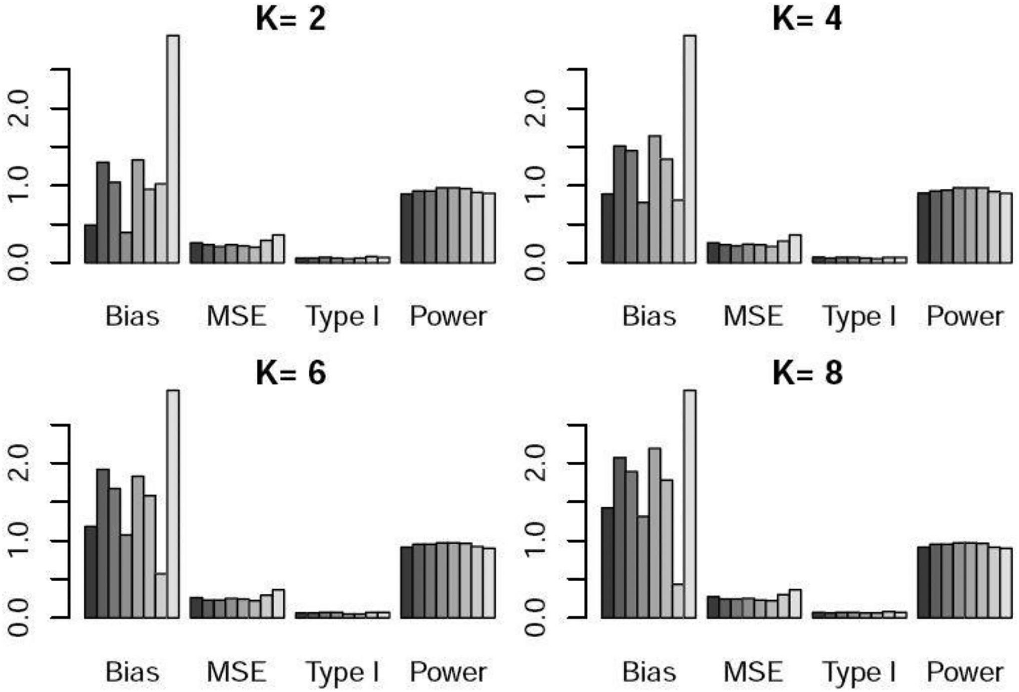
Bias×100, MSE×100, type I error, and power under scenario 2 when the control arm sample size is 150. For each metric, the six bars from left to right respectively represent the WR and DR approaches using logistic regression, GBM, and CBPS, time machine (TM), and the robust meta-analysis-predictive prior approach (RMAP).
Table 2 and Figures S1–S3 shows the performance of the methods when the control arm sample size is 300. Similarly to Table 1, DR yielded slightly lower power than WR when there was no temporal effect and similar power when there was temporal effect. TM gave much lower power for scenario 3 when was large, and RMAP resulted in much higher bias.
3.3. Sensitivity Analyses
We evaluated the performance of our methods in the presence of unmeasured confounders. We considered both linear and non-linear temporal effects (scenarios 4 and 5). We assumed the covariate had a dimension of 6 and followed a multivariate normal distribution , where was a 6 × 6 matrix with diagonal elements 0.25 and off diagonal elements 0.025. The binary outcome was generated from model (6). In scenario 4, , and for . In scenario 5, , and for . We assumed the sixth covariate was an unmeasured confounder, and so in the trial only the first five covariates were used to map non-concurrent controls to the current population and to do the analysis.
Table 3 and Figures 4–5 show the performance of WR, DR, and TM when the control arm sample size is 150. For scenario 4 with linear time trend, DR and WR with GBM and CBPS yielded higher power than TM. When comparing WR and DR, DR yielded lower type I error and higher power on average. In scenario 5, DR provided much higher power than WR and TM. In particular, when , DR resulted in roughly 30% higher power than TM and 10% higher power than WR, demonstrating the advantage of our proposed methods-especially DR when unmeasured confounders are present. Similar patterns can be observed in Table 4 and Figures S4–S5 when the control arm sample size is 300.
Table 3.
Sensitivity analysis in the presence of unmeasured confounders. Bias×100, MSE×100, type I error, and power for the weighted regression (WR) approach and doubly robust (DR) estimator with the propensity score estimated using logistic regression, GBM, and CBPS, time machine (TM) when the control arm sample size is 150.
| K=2 | K=4 | K=6 | K=8 | |||||||||||||
|---|---|---|---|---|---|---|---|---|---|---|---|---|---|---|---|---|
| Bias | MSE | Type I | Power | Bias | MSE | Type I | Power | Bias | MSE | Type I | Power | Bias | MSE | Type I | Power | |
| Scenario 4 | ||||||||||||||||
| WR Logist | −1.79 | 0.25 | 0.07 | 0.88 | −1.88 | 0.26 | 0.07 | 0.88 | −1.96 | 0.27 | 0.06 | 0.87 | −2.03 | 0.27 | 0.06 | 0.88 |
| WR GBM | −2.27 | 0.23 | 0.07 | 0.90 | −2.39 | 0.24 | 0.06 | 0.91 | −2.38 | 0.24 | 0.06 | 0.91 | −2.76 | 0.25 | 0.08 | 0.92 |
| WR CBPS | −2.32 | 0.23 | 0.07 | 0.92 | −2.47 | 0.23 | 0.07 | 0.93 | −2.53 | 0.24 | 0.07 | 0.92 | −2.61 | 0.24 | 0.08 | 0.93 |
| DR Logist | −1.66 | 0.24 | 0.05 | 0.93 | −1.86 | 0.25 | 0.05 | 0.94 | −1.88 | 0.25 | 0.05 | 0.94 | −1.93 | 0.26 | 0.05 | 0.94 |
| DR GBM | −2.47 | 0.24 | 0.05 | 0.93 | −2.35 | 0.24 | 0.06 | 0.92 | −2.61 | 0.26 | 0.05 | 0.93 | −2.67 | 0.25 | 0.06 | 0.92 |
| DR CBPS | −2.16 | 0.22 | 0.04 | 0.92 | −2.32 | 0.23 | 0.04 | 0.92 | −2.37 | 0.23 | 0.04 | 0.92 | −2.46 | 0.24 | 0.04 | 0.92 |
| TM | −0.67 | 0.25 | 0.06 | 0.86 | −0.44 | 0.25 | 0.06 | 0.86 | −0.26 | 0.26 | 0.06 | 0.85 | −0.14 | 0.27 | 0.05 | 0.85 |
| Scenario 5 | ||||||||||||||||
| WR Logist | −1.12 | 0.21 | 0.05 | 0.74 | −1.31 | 0.25 | 0.05 | 0.72 | −1.39 | 0.25 | 0.06 | 0.71 | −1.40 | 0.25 | 0.06 | 0.71 |
| WR GBM | −1.51 | 0.20 | 0.06 | 0.77 | −1.42 | 0.22 | 0.06 | 0.76 | −1.59 | 0.21 | 0.05 | 0.76 | −1.62 | 0.21 | 0.05 | 0.77 |
| WR CBPS | −1.47 | 0.18 | 0.06 | 0.79 | −1.65 | 0.20 | 0.06 | 0.79 | −1.71 | 0.21 | 0.06 | 0.78 | −1.76 | 0.21 | 0.06 | 0.78 |
| DR Logist | −0.96 | 0.21 | 0.07 | 0.86 | −1.21 | 0.25 | 0.07 | 0.87 | −1.29 | 0.25 | 0.07 | 0.87 | −1.30 | 0.25 | 0.07 | 0.87 |
| DR GBM | −1.32 | 0.20 | 0.07 | 0.85 | −1.40 | 0.22 | 0.07 | 0.84 | −1.56 | 0.23 | 0.08 | 0.83 | −1.53 | 0.22 | 0.07 | 0.85 |
| DR CBPS | −1.25 | 0.18 | 0.06 | 0.85 | −1.49 | 0.20 | 0.06 | 0.84 | −1.54 | 0.21 | 0.06 | 0.84 | −1.57 | 0.21 | 0.06 | 0.85 |
| TM | −0.09 | 0.25 | 0.05 | 0.71 | 0.89 | 0.29 | 0.04 | 0.65 | 1.48 | 0.31 | 0.04 | 0.62 | 1.93 | 0.34 | 0.04 | 0.58 |
Fig. 4.
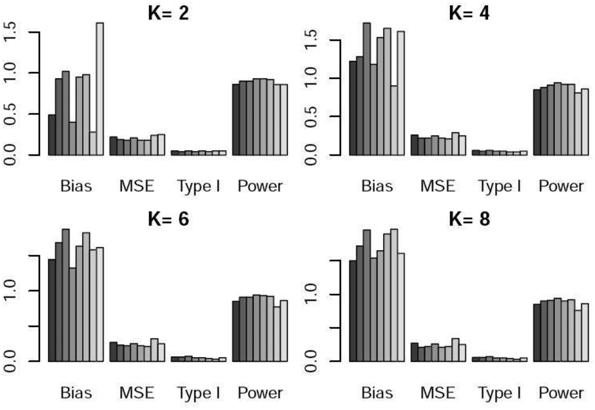
Bias×100, MSE×100, type I error, and power under scenario 3 when the control arm sample size is 150. For each metric, the six bars from left to right respectively represent the WR and DR approaches using logistic regression, GBM, and CBPS, time machine (TM), and the robust meta-analysis-predictive prior approach (RMAP).
Fig. 5.
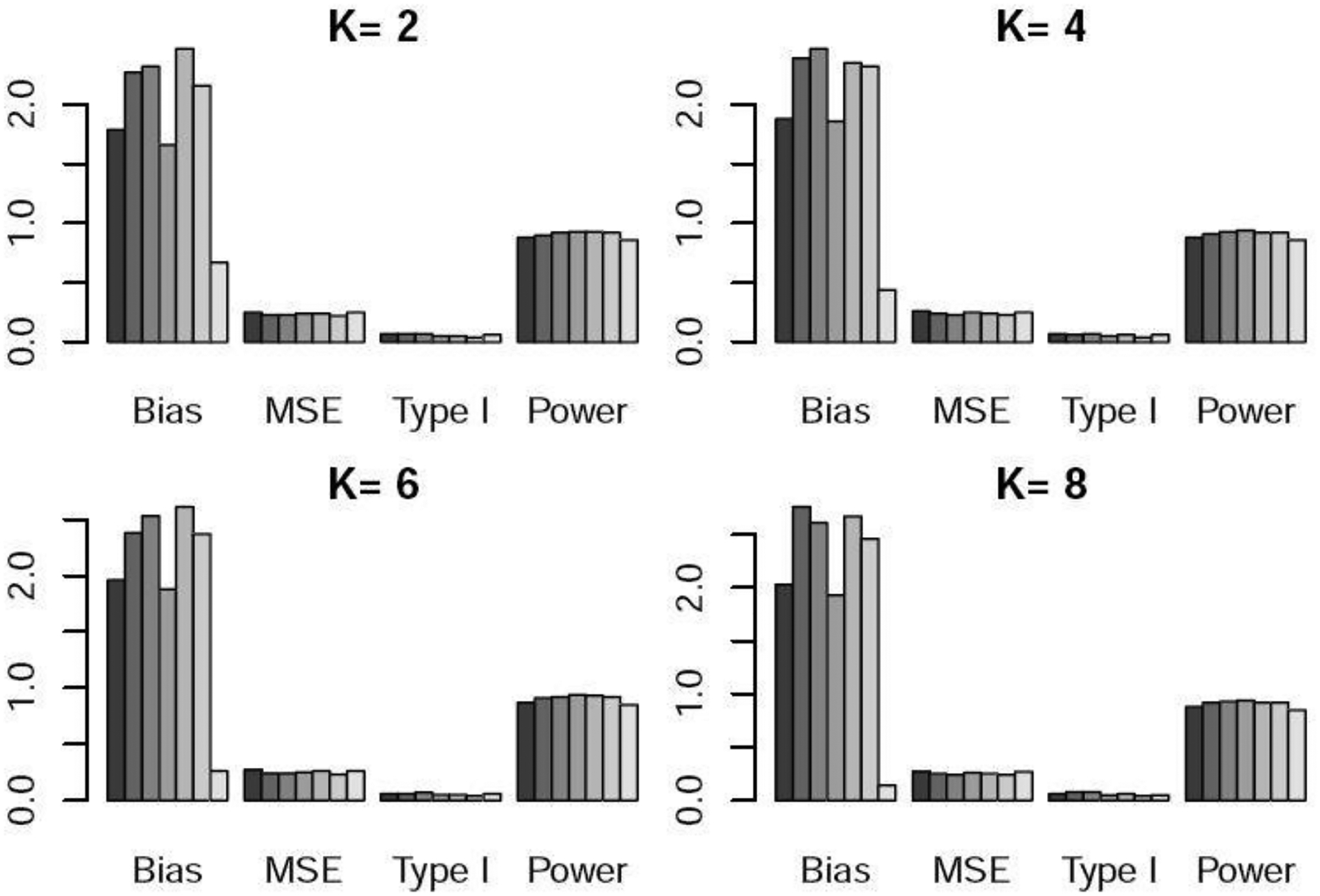
Bias×100, MSE×100, type I error, and power under scenario 4 when the control arm sample size is 150. For each metric, the six bars from left to right respectively represent the WR and DR approaches using logistic regression, GBM, and CBPS, time machine (TM), and the robust meta-analysis-predictive prior approach (RMAP).
Table 4.
Sensitivity analysis in the presence of unmeasured confounders. Bias×100, MSE×100, type I error, and power for the weighted regression (WR) approach and doubly robust (DR) estimator with the propensity score estimated using logistic regression, GBM, and CBPS, time machine (TM) when the control arm sample size is 300.
| K=2 | K=4 | K=6 | K=8 | |||||||||||||
|---|---|---|---|---|---|---|---|---|---|---|---|---|---|---|---|---|
| Bias | MSE | Type I | Power | Bias | MSE | Type I | Power | Bias | MSE | Type I | Power | Bias | MSE | Type I | Power | |
| Scenario 4 | ||||||||||||||||
| WR Logist | −1.82 | 0.14 | 0.07 | 0.96 | −1.90 | 0.14 | 0.07 | 0.95 | −1.98 | 0.14 | 0.07 | 0.96 | −2.05 | 0.15 | 0.07 | 0.96 |
| WR GBM | −2.20 | 0.15 | 0.07 | 0.96 | −2.21 | 0.15 | 0.08 | 0.96 | −2.22 | 0.14 | 0.07 | 0.96 | −2.40 | 0.15 | 0.08 | 0.97 |
| WR CBPS | −2.15 | 0.14 | 0.07 | 0.97 | −2.38 | 0.14 | 0.08 | 0.97 | −2.49 | 0.15 | 0.08 | 0.98 | −2.54 | 0.15 | 0.08 | 0.97 |
| DR Logist | −1.67 | 0.13 | 0.05 | 0.95 | −1.77 | 0.14 | 0.05 | 0.95 | −1.85 | 0.14 | 0.06 | 0.95 | −1.87 | 0.15 | 0.05 | 0.95 |
| DR GBM | −2.15 | 0.14 | 0.05 | 0.95 | −2.17 | 0.15 | 0.06 | 0.95 | −2.20 | 0.15 | 0.05 | 0.94 | −2.17 | 0.14 | 0.06 | 0.94 |
| DR CBPS | −2.01 | 0.13 | 0.05 | 0.95 | −2.22 | 0.14 | 0.05 | 0.95 | −2.31 | 0.14 | 0.05 | 0.94 | −2.36 | 0.15 | 0.05 | 0.94 |
| TM | −0.65 | 0.15 | 0.07 | 0.94 | −0.56 | 0.15 | 0.06 | 0.94 | −0.48 | 0.15 | 0.06 | 0.94 | −0.39 | 0.16 | 0.06 | 0.94 |
| Scenario 5 | ||||||||||||||||
| WR Logist | −1.10 | 0.11 | 0.06 | 0.86 | −1.21 | 0.13 | 0.06 | 0.83 | −1.35 | 0.13 | 0.06 | 0.85 | −1.37 | 0.14 | 0.06 | 0.84 |
| WR GBM | −1.31 | 0.11 | 0.05 | 0.87 | −1.49 | 0.13 | 0.06 | 0.86 | −1.45 | 0.12 | 0.05 | 0.85 | −1.68 | 0.13 | 0.06 | 0.86 |
| WR CBPS | −1.32 | 0.10 | 0.06 | 0.88 | −1.61 | 0.12 | 0.06 | 0.88 | −1.70 | 0.12 | 0.06 | 0.89 | −1.72 | 0.12 | 0.06 | 0.88 |
| DR Logist | −0.87 | 0.10 | 0.06 | 0.88 | −1.08 | 0.13 | 0.07 | 0.89 | −1.20 | 0.13 | 0.07 | 0.89 | −1.26 | 0.13 | 0.07 | 0.89 |
| DR GBM | −1.23 | 0.10 | 0.06 | 0.87 | −1.42 | 0.12 | 0.06 | 0.87 | −1.38 | 0.12 | 0.06 | 0.86 | −1.39 | 0.13 | 0.07 | 0.88 |
| DR CBPS | −1.13 | 0.09 | 0.06 | 0.87 | −1.47 | 0.11 | 0.06 | 0.87 | −1.55 | 0.12 | 0.06 | 0.87 | −1.58 | 0.12 | 0.06 | 0.88 |
| TM | −0.24 | 0.14 | 0.05 | 0.84 | 0.85 | 0.17 | 0.04 | 0.78 | 1.36 | 0.18 | 0.03 | 0.76 | 1.70 | 0.20 | 0.03 | 0.74 |
4. Discussion
We have proposed two approaches to adjust for temporal drift in adaptive platform trials. A frequentist weighted regression approach relies on the propensity score model being correctly specified. The Bayesian weighted regression with smoothed time effects is doubly robust in the sense that the treatment comparisons are valid if either the propensity score model is correctly specified or if the time-effect model is correctly specified. Our proposed approaches use information in both the response variable and the covariates. Simulation study shows that these methods have desirable operating characteristics and that they outperform alternative methods in the case of non-linear time effects or unmeasured confounders. When there is no unmeasured confounder, the doubly robust approach yields similar performance with the frequentist weighted regression approach. When there are unmeasured confounders, the doubly robust approach has higher power.
In this paper, we consider continuous or binary response variables. Our methods can be extended to time-to-event outcomes or late-onset outcomes. In the doubly robust Bayesian weighted regression approach, we divide the time period into subintervals and model the time effect on each subinterval. An alternative approach is to use splines to model the smoothed time effect over the whole time region. Instead of using propensity score weighting to map non-concurrent controls to concurrent data, a parallel approach is to use propensity score matching, which is one of the most commonly used approaches to incorporate historical control data in clinical trials. These are topics of our future research.
Supplementary Material
Fig. 2.
Bias×100, MSE×100, type I error, and power under scenario 1 when the control arm sample size is 150. For each metric, the six bars from left to right respectively represent the WR and DR approaches using logistic regression, GBM, and CBPS, time machine (TM), and the robust meta-analysis-predictive prior approach (RMAP).
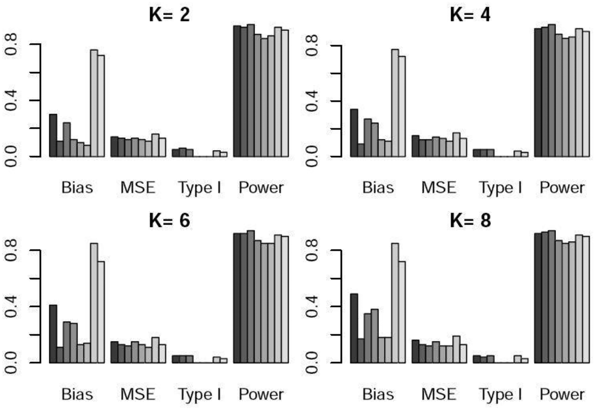
Fig. 6.

Bias×100, MSE×100, type I error, and power under scenario 5 when the control arm sample size is 150. For each metric, the six bars from left to right respectively represent the WR and DR approaches using logistic regression, GBM, and CBPS, time machine (TM), and the robust meta-analysis-predictive prior approach (RMAP).
Acknowledgement
The authors thank the Associate Editor and two Referees for their valuable comments which substantially improved the presentation of this article. Guo’s research is supported by the R & D Research Competitiveness Subprogram of Louisiana Board of Regents, Contract number LEQSF(2022-25)-RD-A-07. Yuan’s research was partially supported by Award Number P50CA221707, P50CA127001 and P30 CA016672 from the National Cancer Institute.
Footnotes
Conflict of Interest
None declared.
References
- Atman D, Royston J (1988), The hidden effect of time. Statistics in Medicine, 7: 629–637. [DOI] [PubMed] [Google Scholar]
- FDA, (2019), Draft guidance for industry: interacting withe the FDA on complex innovative trial designs for drug and biological products cancer vaccines.
- Hobbs B, Carlin B, Mandrekar S, Sargent D (2011), Hierarchical commensurate and power prior models for adaptive incorporation of historical information in clinical trials. Biometrics, 67, 1047–1056. [DOI] [PMC free article] [PubMed] [Google Scholar]
- Hobbs B, Chen N, Lee J (2018), Controlled multi-arm platform design using predictive probability. Statistical Methods in Medical Research, 27: 65–78. [DOI] [PMC free article] [PubMed] [Google Scholar]
- Ibrahim J, Chen M, Gwon Y, Chen F (2015), The power prior: theory and applications. Statistics in Medicine, 34, 3742–3749. [DOI] [PMC free article] [PubMed] [Google Scholar]
- Imai K, Ratkovic M (2014), Covariate balancing propensity score. Journal of the Royal Statistical Society, 76, 243–263. [Google Scholar]
- Imbens GW, Rubin DB (2015), Causal inference for statistics, Social and biomedical science: an introduction, New York: Cambridge University Press. [Google Scholar]
- Kaizer A, Hobbs B, Koopmeiners J (2018), A multi-source adaptive platform design for testing sequential combinatorial therapeutic strategies. Biometrics, 74: 1082–1094. [DOI] [PMC free article] [PubMed] [Google Scholar]
- Lee K, Wason J (2020), Including non-concurrent control patients in the analysis of platform trials: is it worth it?. BMC Med Res Methodol, 20: 165. [DOI] [PMC free article] [PubMed] [Google Scholar]
- Li F, Morgan K, Zaslavsky A (2018), Balancing covariates via propensity score weighting. Journal of the American Statistician Association, 113: 390–400. [Google Scholar]
- Lipsky A, Greenland S (2011), Confounding due to changing background risk in adaptively randomized trials. Clinical Trials, 8: 390–397. [DOI] [PMC free article] [PubMed] [Google Scholar]
- Meyer E, Mesenbrink Pl, Dunger-Baldauf C, et al. , (2020), The evolution of master protocol clinical trial designs: a systematic literature review. Clinical Therapeutics, 42: 1330–60. [DOI] [PubMed] [Google Scholar]
- McCaffrey D, Ridgeway G, Morral A (2004), Propensity score estimation with boosted regression for evaluating causal effects in observational studies. Psychological Methods, 9, 403–425. [DOI] [PubMed] [Google Scholar]
- McCaffrey D, Griffin B, Almirall D, Slaughter M, Ramchand R, Burgette L (2013), A Tutorial on Propensity Score Estimation for Multiple Treatments Using Generalized Boosted Models, 32, 3388–3414. [DOI] [PMC free article] [PubMed] [Google Scholar]
- Neuenschwander B, Capkun-Niggli C, Branson M, Spiegelhalter D, (2010), Summarizing historical information on controls in clinical trials. Clinical Trials, 7, 5–18. [DOI] [PubMed] [Google Scholar]
- Rosenbaum PR, Rubin DB (1983), Assessing sensitivity to an unobserved binary covariate in an observational study with binary outcome. The Journal of the Royal Statistical Society, B, 45, 212–218. [Google Scholar]
- Rubin DB (1974), Estimating causal effects of treatments in randomized and nonrandomized studies. Journal of Educational Psychology, 66, 688–701. [Google Scholar]
- Rubin DB (1978), Bayesian inference for Causal effects: the role of randomization. The Annals of Statistics, 6, 34–58. [Google Scholar]
- Rubin DB (1980), Comment on “Randomization Analysis of Experimental Data: the Fisher randomization test” by D. Basu, Journal of the American Statistical Association, 75, 591–593. [Google Scholar]
- Saville B, Berry S (2016), Efficiencies of platform clinical trials: a vision of the future. Clinical Trials, 13: 358–366. [DOI] [PubMed] [Google Scholar]
- Saville B, Berry D, Berry N, Niele K, Berry S (2022), The Bayesian time machine accounting for temporal drift in multi-arm platform trials. Clinical Trials, In Press. [DOI] [PubMed] [Google Scholar]
- Schmidli H, Gsteiger S, Roychoudhury S, O’Hagan A, Spiegelhalter D, Neuenschwander B, (2014), Robust meta-analytic-predictive priors in clinical trials with historical control information. Biometrics, 70, 1023–1032. [DOI] [PubMed] [Google Scholar]
- Spiegelhalter D, Albrams K, Myles J, (2004), Bayesian approaches to Clinical trials and health-care evaluation. Chichester: Wiley. [Google Scholar]
- Vittinghoff E, McCulloch C (2006), Relaxing the Rule of Ten Events per Variable in Logistic and Cox Regression. American Journal of Epidemiology, 165, 710–718. [DOI] [PubMed] [Google Scholar]
- Wang C, Lin M, Gary R, Soon G, (2022), A Bayesian model with application for adaptive platform trials having temporal changes. Biometrics, In Press. [DOI] [PubMed] [Google Scholar]
- Wang C, Li H, Chen W, Lu N, Tiwari R, Xu Y, Yue Li. (2019), Propensity score-integrated power prior approach for incorporating real-world evidence in single-arm clinical studies. JOURNAL OF BIOPHARMACEUTICAL STATISTICS, 29, 731–748. [DOI] [PubMed] [Google Scholar]
- Woodcock M, LaVange L (2017), Master protocols to study multiple therapies, multiple diseases, or both. The New England Journal of Medicine, 377, 62–70. [DOI] [PubMed] [Google Scholar]
- Yang P, Zhao Y, Nie L, Vallejo J, Yuan Y (2023), SAM: Self-adapting mixture prior to dynamically borrow information from historical data in clinical trials. https://arxiv.org/abs/2305.12279. [DOI] [PMC free article] [PubMed]
- Yuan Y, Xia J, et al. (2017), A calibrated power prior approach to borrow information from historical data with application to biosimilar clinical trials. Journal of the Royal Statistical Society, Series C, 66,979. [DOI] [PMC free article] [PubMed] [Google Scholar]
- Yuan Y, Guo B, Munsell M, Lu K, Jazaeri A (2016), MIDAS: a practical Bayesian design for platform trials with molecularly targeted agents. Statistics in Medicine, 35: 3892–3906. [DOI] [PMC free article] [PubMed] [Google Scholar]
Associated Data
This section collects any data citations, data availability statements, or supplementary materials included in this article.