Scanorama: Integrating large and diverse single-cell transcriptomic datasets

Abstract

Merging diverse single-cell RNA sequencing (scRNA-seq) data from numerous experiments, laboratories, and technologies can uncover significant biological insights. Nonetheless, integrating scRNA-seq data encounters special challenges when the datasets are composed of diverse cell type compositions. Scanorama offers a robust solution for improving the quality and interpretation of heterogeneous scRNA-seq data by effectively merging information from diverse sources. Scanorama is designed to address the technical variation introduced by differences in sample preparation, sequencing depth, and experimental batches that can confound the analysis of multiple scRNA-seq datasets. Here, we provide a detailed protocol for using Scanorama within a Scanpy-based single cell analysis workflow coupled with Google Colaboratory, a cloud-based free Jupyter notebook environment service. The protocol involves Scanorama integration, a process that typically spans 0.5 to 3 hours. Scanorama integration requires a basic understanding of cellular biology, transcriptomic technologies, and bioinformatics. Our protocol and new Scanorama-Colab resource should make scRNA-seq integration more widely accessible to researchers.

Editorial summary:

Scanorama is an effective tool for combining multiple scRNA-seq datasets, addressing technical variation introduced by differences in sample preparation, sequencing depth, and experimental batches that can confound the analysis of diverse datasets.

Proposed tweet:

Scanorama: Integrating large and diverse single-cell transcriptomic datasets @brianhie @SoochiKim @Thomas_Rando @thebrysonlab @lab_berger

Proposed teaser:

Scanorama: Integrating scRNA-seq datasets

Introduction

There has been a substantial increase in both the quantity and scale of single-cell RNA sequencing (scRNA-seq) studies. Two global initiatives, the Tabula Sapiens Consortium¹ and the Human Cell Atlas², have made significant contributions to understanding multiple organs and tissues at the single cell level. Researchers from diverse areas of expertise have dedicated considerable effort to collecting, profiling, and analyzing data from these organs and tissues, resulting in vast, comprehensive collections of scRNA-seq datasets that are freely accessible to the scientific community. scRNA-seq studies aim to map and understand the cellular landscape of multiple organs and tissues at a single-cell resolution. However, one of the major challenges of analyzing multiple scRNA-seq datasets is the presence of batch effects that stem from technical or biological factors (see Glossary in Box 1), making it difficult to distinguish biologically meaningful differences across datasets³.

Box 1: Glossary.

Sequencing depth: The number of sequencing reads obtained from a sample during an RNA sequencing experiment. It indicates how many times a specific region of the transcriptome is sequenced, providing an estimate of the abundance or expression level of the corresponding genetic elements.

Latent space: A lower-dimensional representation of the data that captures its underlying structure or patterns³⁶. Scanorama utilizes a dimensionality reduction technique that leverages the singular value decomposition to compress the gene expression profiles of each cell.

Technical variation: The variability in experimental measurements that arises from technical sources rather than biological sources. This includes, sample processing, library preparation, sequencing, and data acquisition.

Batch effect: The systematic variation in experimental measurements that arises from technical or non-biological sources due to differences in sample processing, experimental conditions, or the result of handling cells in distinct groups or ‘batches’.

Integration: The process of combining or merging multiple scRNA-seq datasets obtained from different experimental conditions, tissues, or platforms into a unified representation.

Batch correction: A data preprocessing technique used in multi-sample or multi-batch experiments to remove or minimize unwanted systematic variations introduced by technical factors or batches in scRNA-seq analysis.

Overcorrection: When the batch correction method removes meaningful biological signal.

Nearest neighbors: A technique used to identify the closest data points to a given data point based on a specified distance metric.

Mutual nearest neighbors: A technique that matches a pair of cells between two datasets if both cells in the pair are within the neighborhood of closest cells when considering the other dataset. This technique is used in the context of comparing and aligning datasets to find similar or corresponding points across datasets.

Dimensionality reduction: The process of reducing the number of variables or features in a dataset to improve computational efficiency and enhance data visualization.

Development of the Protocol

Accurate integration of heterogeneous collections of scRNA-seq data is the critical step for overcoming technical and biological challenges. To address this issue, many methods have been developed to integrate and batch correct multiple scRNA-seq datasets^4–8. Alongside several methods such as Batch-Balanced k-Nearest Neighbors (BBKNN)⁸ and deep learning models such as single-cell variational inference (scVI)⁹ and single-cell annotation using variational inference (scANVI)¹⁰, Scanorama has emerged as one of the leading tools for scRNA-seq data integration. Scanorama is highly efficient and accurate in removing batch effects, can handle multiple batches and dataset types, and is less prone to overcorrection, preserving biologically relevant differences across datasets^{3, 11, 12}. Moreover, Scanorama can avoid overcorrection when a dataset has no overlapping cell types with any other dataset, making it a preferred choice for batch correction of heterogeneous and complex datasets¹¹. In a previous study¹¹, we presented Scanorama’s efficacy across diverse datasets. Here, present an updated and detailed protocol for Scanorama, integrating it into a Scanpy-based single cell analysis workflow on Google Colaboratory, enhancing its accessibility and usability.

Our protocol was originally developed using the mutual-nearest-neighbors matching strategy proposed by Haghverdi et al.⁴ for aligning cell types across two datasets. We extended this to account for alignments across many datasets, alongside algorithmic and software optimizations to improve computational efficiency. We later developed an additional method, Geometric Sketching (Geosketch), which intelligently downsamples single-cell datasets and allows Scanorama to conduct its most resource-intensive alignment step on a small subsample of the dataset while still applying the integration to the full dataset, resulting in a substantial speed-up of the entire process.

Overview of the Procedure

Here we describe a protocol to integrate multiple scRNA-seq datasets, spanning from small to large-scale scenarios, using Scanorama in a Jupyter Notebook inside Google Colaboratory. This protocol enables researchers to remove batch effects and perform downstream analysis on integrated datasets, providing a valuable resource for understanding cellular processes at single-cell resolution.

Expected inputs

Scanorama takes in a single-cell dataset in which the cells belong to different batches. In our protocol, we use the AnnData format to store the dataset. AnnData also allows the user to specify a “batch_variable” that indicates which cells belong to which batch.

Expected outputs

Scanorama produces a low-dimensional embedding or representation of each cell, where the distances among the cells within this embedding space aim to better represent the biological diversity of the data without the confounding batch effects that may be present in the original data. This low dimensional embedding can be used as input to further downstream analysis such as visualization and clustering.

Prepare Scanorama inputs (Steps 1–6)

The initial steps of the Scanorama integration protocol involves setting up a connection to a computer with internet access, launching a Jupyter notebook in Google Colaboratory, and connecting to the Colab’s run time. Following this, a user creates a directory and downloads datasets. Our protocol then details the essential packages to install and import, including Scanorama and Scanpy. The subsequent steps encompass loading Scanorama input datsets, as AnnData objects. In our protocol, we illustrate how different datasets can be processed by Scanorama by providing three datasets of different sizes as potential input. Users can also incorporate their own datasets by uploading or downloading AnnData objects of interest to the created directory.

Scanorama integration (Step 7 and 10)

Scanorama integration in the protocol is marked by two key processes. Firstly, AnnData objects are split by batch, generating a list of AnnData representing individual batches over which the user desires to apply integration. Choosing an appropriate batch key in Scanorama integration is crucial, as it significantly influences the grouping and processing of datasets. The selection of a batch key depends on various factors, including its biological relevance, representation of technical variations, and alignment with the experimental design. We highly recommend users to explore the dataset, visualize metadata features, and understand how well they correspond to expected batch variations. Secondly, the Scanorama-corrected matrix is incorporated into the original AnnData object. A new AnnData object (‘adata_sc’) is created as a copy of the initial dataset, and the corrected matrices obtained from individual batches are aggregated and added to the ‘Scanorama’ key in the object’s observation matrix (‘obsm’).

Optional steps to accelerate Scanorama integration (Steps 8–9 and 12–14)

We’ve also included the optional steps, which are designed for more complex and large dataset integration. First, highly variables genes are identified in the merged dataset, focusing on the specified ‘batch_key’ and ensuring selection of genes variable in at least two batches. Subsequently, the individual AnnData objects are subset to encompass only these variable genes, improving efficiency by reducing the number of genes to consider. The core integration process is then performed using Scanorama as in Scanorama integration step, with the integrated result stored back in the ‘adatas’ variable as ‘X_scanorama’. For those seeking to accelerate integration further, Scanorama introduces the ‘sketch_method’ parameter, particularly leveraging the Geosketch¹³ method for efficient integration of large datasets. Users are encouraged to explore the impact of Geosketch parameters via the provided Colab notebook, conducting tests with varying sketch sizes. We’ve also included a benchmarking analysis, assessing the impact of subsampling on Scanorama integration using 10 metrics from scib-metrics³. The results are visualized in a comprehensive table, providing valuable insights into the integration performance.

Visualize batch correction (Steps 15–17)

To assess the impact of batch correction on the structure of the scRNA-seq data, a series of steps, including computing the k-nearest-neighbors graph and performing dimensionality reductions such as t-SNE and UMAP, are conducted on the integrated dataset. This allows for clustering and visualization of the corrected data. Simultaneously, uncorrected data is prepared for comparison by applying similar dimensionality reduction steps.

Assess Scanorama integration quality (Steps 18–23)

In this last step, we aim to evaluate the quality of integration by assessing the consistency between Leiden cluster labels and various metadata label keys. The steps involve installing the necessary packages and running the Leiden algorithm for clustering analysis. Mutual information scores are then calculated between Leiden clusters and specified metadata label keys. We have also included optional steps to provide further insights into Scanorama’s performance, allowing users to optimize parameters, benchmark against other methods, and assess resource consumption.

Comparison with other methods

Batch correction methods for scRNA-seq data can be categorized into four broad categories: global models¹⁴, nearest-neighbor methods^{4–7, 11}, graph-based methods⁸ and deep learning approaches^{9, 10, 15}. However, these methods face common challenges, such as overcorrection, the use of latent space for integration, and difficulty in disentangling batch effects from the underlying biological signal of interest. Scanorama belongs to the category of nearest-neighbor methods, utilizing approximate nearest neighbor search techniques based on locality-sensitive hashing and random projection trees^{11, 16}. Scanorama has been shown to perform well at integrating across heterogeneous datasets while still taking a more conservative approach to removing inter-dataset variation, which typically leads to better preservation of biological signal¹¹.

Multiple benchmarks have been conducted to evaluate the performance of various batch correction and data integration methods^{3, 17,18}. A recent comprehensive benchmark called scib-metrics, which also implements a usable software package for conducting comparisons of single-cell integration methods, highlighted that Scanorama is among the top-performing methods, along with deep learning approaches scANVI, scVI, and scGen, particularly for complex tasks that involve multiple datasets and high biological complexity³. When choosing a method, it is important to evaluate the integration performance using appropriate metrics and evaluation pipelines and to test multiple methods before selecting the most appropriate one. Scanorama’s ability to handle multiple batches and dataset types while efficiently and accurately removing batch effects and identifying biologically relevant differences across datasets make it a compelling option for scRNA-seq data integration.

Challenges and limitations

There are some limitations and challenges that are important to keep in mind when using Scanorama or performing data integration of scRNA-seq datasets more generally. Scanorama employs a few algorithm approximations to improve computational efficiency. Scanorama compresses the gene expression profiles of cells into a low-dimensional embedding using an efficient randomized singular value decomposition (SVD)¹⁹. This step improves the robustness to noise, but results in a loss of information, and may inadvertently remove or blur genuine biological differences between batches. Scanorama also utilizes approximate nearest neighbor search techniques based on locality sensitive hashing and random projection trees^{16, 20}. This assumes a shared subpopulation structure among the integrated datasets. While this reduces query time and makes batch correction feasible for large-scale datasets, it may lose accuracy compared to exact nearest neighbor search. Scanorama’s computational requirements can also be reduced by limiting the number of batch-corrected genes by targeting analysis only to highly variable genes or through downsampling the number of cells used to perform mutual-nearest-neighbors matches among datasets¹³.

When large differences exist between batches or datasets, Scanorama employs a conservative mutual-nearest-neighbors matching algorithm and may not completely separate these effects, potentially leading to incomplete integration. On the other hand, Scanorama does transform the underlying data and may also therefore remove biologically meaningful differences. One approach to assessing problems of under- or overcorrection is to use ground-truth standards (for example, cells that are known to be of the same or different cell types) across datasets. Assessing the accuracy of batch correction methods can be challenging in the absence of a ground truth. While Scanorama and other methods can improve alignment between datasets, the true underlying biological heterogeneity and the extent of batch effects may remain uncertain. Researchers should consider these limitations, evaluate the suitability of Scanorama or alternative methods based on their specific scRNA-seq dataset and research question, and leverage comparative evaluations, benchmarking studies, and validation on gold standard datasets to assess performance and appropriateness of batch correction methods in different scenarios.

Experimental Design

The use of single-cell integration requires several important considerations. As detailed in the previous section, proper integration should consider the use of positive and negative controls to assess the impact of under- or over-correction. Another important consideration is the selection of the batch variable, as Scanorama is encouraged to remove differences between cells with different batch labels.

Our Scanorama protocol is designed to be generally applicable to different collections of scRNA-seq datasets. We build off of the commonly used AnnData format and the user needs only to provide Scanorama with a single AnnData object that contains the data and the user-specified batch variable.

Users with large datasets and limited computational resources should consider running Scanorama integration with sketch-based acceleration, which is described in our protocol. Using sketching with Scanorama simply requires providing a parameter to Scanorama that turns on this functionality, as well as a parameter specifying the desired sketch size (smaller values will result in faster integration but will also potentially lead to decreased sensitivity to biological variation and therefore poorer performance).

Materials

Equipment

• A computer with internet connection.

• Google Colab account; this workflow has been tested on Colab Pro+ account. Colab Pro or Colab Pro+ options are recommended for large dataset integration. For more information, please refer to https://colab.research.google.com/.

Software

• Scanorama¹¹ installation: Installation instruction can be found at https://github.com/brianhie/scanorama

• Scanpy²¹ installation: Installation instructions can be found at https://github.com/scverse/scanpy

• Pandas installation: Installation instructions can be found at https://github.com/pandas-dev/pandas

• Numpy²² installation: Installation instructions can be found at https://github.com/numpy/numpy

• Matplotlib installation: Installation instructions can be found at https://github.com/matplotlib/matplotlib

• Anndata²³ installation: Installation instructions can be found at https://github.com/scverse/anndata

Datasets

• Small dataset example: 293T cells, Jurkat cells, and a 50:50 293T:Jurkat mixture.

• Large dataset 1 example: 26 datasets from 9 different technologies. Both of these datasets (Small dataset and Large dataset 1) are used in original study¹¹ and are available from:

• https://zenodo.org/record/7968485

• Large dataset 2 example: Tabula Sapiens¹ transcriptomic cell atlas individual organ datasets from human fat, muscle and blood. In total, there are 46 cell ontology classes represented in these datasets, with only 2 overlapping cell ontology classes across all three objects, and each tissue object has unique cell ontology classes, with 19 in blood, 5 in fat, and 11 in muscle. All processed datasets used in this example and other organs are available from:

  https://figshare.com/articles/dataset/Tabula_Sapiens_release_1_0/14267219

Procedures

Prepare example Scanorama inputs.

• 1[1 minute] To get started, establish a connection to a computer that has an internet connection and launch a new Jupyter notebook using Google Colaboratory (Colab) or open example notebook using the links below. Make sure to connect to the runtime and, if have a Colab Pro/Pro+ subscription, enable high memory (High-RAM) as needed to accelerate the integration processes and minimize the risk of hitting usage limits when working with large datasets. ?TROUBLESHOOTING
  Below, we use prepared example datasets as input to Scanorama. Users can use their own datasets by creating an AnnData object (adata) that includes a “batch_key” in the AnnData’s observation metadata (adata.obs)

  • Colab notebook for small dataset (293T and Jurkat) example: https://colab.research.google.com/drive/12hNry9nlMgZRu-bGUiXbz0Veqeh2WhcU?usp=sharing
  • Colab notebook for large dataset 1 (26 datasets) example: https://colab.research.google.com/drive/1OZrdeT1ob2FSSgTSK8Qa3hijoW1bb9Y3?usp=sharing
  • Colab notebook for large dataset 2 (Tabula Sapiens datasets) example: https://colab.research.google.com/drive/1X6ssJI9jTzqRJ9QQ44YffSvUhnlv2kR7?usp=sharing
• 2
  [1 minute] Create a directory for downloading and unpacking datasets. Enter the following command in the Jupyter notebook to make a directory.

  !mkdir –p /content/drive/MyDrive/<directory name>
  

• 3
  [5–15 minutes] Download and unpack datasets for Scanorama integration.

  #####- Small datasets -#####
  !wget -P /content/drive/MyDrive/<directory name>
  https://zenodo.org/record/7968485/files/small_dataset.zip
  !unzip /content/drive/MyDrive/<directory name>/small_dataset.zip -d /content/drive/MyDrive/<directory name>
  #####- Large dataset 1 -#####
  !wget -P /content/drive/MyDrive/<directory name>
  https://zenodo.org/record/7968485/files/large_dataset.zip
  !unzip /content/drive/MyDrive/<directory name>/large_dataset.zip -d /content/drive/MyDrive/<directory name>
  #####- Large dataset 2: Fat, Muscle and Blood AnnData objects -#####
  !wget -O /content/drive/MyDrive/<directory name>/TS_Fat.h5ad.zip https://figshare.com/ndownloader/files/34701973
  !wget -O /content/drive/MyDrive/<directory name>/TS_Muscle.h5ad.zip https://figshare.com/ndownloader/files/34702000
  !wget -O /content/drive/MyDrive/<directory name>/TS_Blood.h5ad.zip https://figshare.com/ndownloader/files/34701964
  !unzip /content/drive/MyDrive/<directory name>/TS_Fat.h5ad.zip -d /content/drive/MyDrive/<directory name>
  !unzip /content/drive/MyDrive/<directory name>/TS_Muscle.h5ad.zip -d /content/drive/MyDrive/<directory name>
  !unzip /content/drive/MyDrive/<directory name>/TS_Blood.h5ad.zip -d /content/drive/MyDrive/<directory name>
  

• 4
  [1 minute] Install and load required packages.

  !pip install scanorama
  !pip install scanpy
  import scanorama
  import scanpy as sc
  import anndata as ad
  import scanpy.external as sce
  import matplotlib.pyplot as plt
  import numpy as np
  

Load Scanorama inputs:

• 5
  [1 minute] Load AnnData objects to integrate using the ‘read_h5ad’ function from the Scanpy package.

  • Load small dataset example:

    adata = sc.read_h5ad(‘/content/drive/MyDrive/<directory name>/small_dataset/small_data_293T_Jurkat.h5ad’)
    

  • Load large dataset 1 example

    adata = sc.read_h5ad(‘/content/drive/MyDrive/<directory name>/large_dataset/large_data_26dataset.h5ad’)
    

  • Load large dataset 2 example

    adata1 = sc.read_h5ad(‘/content/drive/MyDrive/<directory name>/TS_Fat.h5ad’)
    adata2 = sc.read_h5ad(‘/content/drive/MyDrive/<directory name>/TS_Muscle.h5ad’)
    adata3 = sc.read_h5ad(‘/content/drive/MyDrive/<directory name>/TS_Blood.h5ad’)
    

• 6
  For any dataset that spans multiple AnnData objects such as large dataset 2, merge and preprocess AnnData objects for integration.

  • [1 minute] First merge AnnData objects using the ‘concatenate’ function from the AnnData package.

    Adata_concat = adata1.concatenate([adata1, adata2], batch_key=‘organ_tissue’, batch_categories=[‘Fat’, ‘Muscle’, ‘Blood’], join=‘outer’)
    

  • [1 minute] Then preprocess the merged objects for integration: extract raw gene expression, normalize total counts to 10,000, and apply natural logarithm transformation to the count matrix.

    adata = sc.AnnData(X=adata_concat.raw.X, var=adata_concat.raw.var, obs = adata_concat.obs)
    sc.pp.normalize_per_cell(adata, counts_per_cell_after=1e4)
    sc.pp.log1p(adata)
    

Scanorama integration.

• 7
  [1 minute] Split AnnData object by batch and create a list of AnnData.

  batch_key = <NAME of BATCH KEY>
  adatas = [adata[adata.obs[batch_key] == batch_value].copy() for batch_value in adata.obs[batch_key].unique()]
  

Optional steps for large dataset integration [Steps 8–9].

• 8
  [1 minute] Identify highly variable genes in the merged dataset, based on the ‘batch_key’ and select the genes that are variable in at least 2 batches. Adjust the code by replacing ‘<NAME of BATCH KEY>‘, ‘<NAME of LABEL KEY>‘ with the actual names of your metadata batch and label keys.

  batch_key = <NAME of BATCH KEY>
  label_key = <NAME of LABEL KEY>
  sc.pp.highly_variable_genes(adata, batch_key = batch_key)
  # Select all genes that are variable in at least 2 batches
  var_select = adata.var.highly_variable_nbatches > 2
  var_genes = var_select.index[var_select]
  

• 9
  [1 minute] Subset the individual AnnData object to contain only the same variable genes.

  adatas = [adata[adata.obs[batch_key] == batch_value][:, var_genes].copy() for batch_value in adata.obs[batch_key].unique()]
  

• 10
  [1–10 minutes] Perform batch correction and integration using Scanorama. The integrated result is stored back in the ‘adatas’ variable as ‘X_scanorama’.

  scanorama.integrate_scanpy(adatas, dimred = 100)
  

  ?TROUBLESHOOTING

• 11
  [1 minute] Add Scanorama corrected matrix to the AnnData object.

  adata_sc = adata.copy()
  scanorama_int = [ad.obsm[‘X_scanorama’] for ad in adatas]
  all_s = np.concatenate(scanorama_int)
  adata_sc.obsm[‘Scanorama’] = all_s
  

Optional parameters for accelerating integration with Geosketch¹³ [Step 12–14].

Scanorama provides an optional parameter called ‘sketch_method’, which is designed to leverage sketching methods for obtaining a compressed representation of a large dataset. This feature is particularly useful to accelerate integration time.

To explore and understand the impact of the Geosketch parameters in Scanorama, please refer to the extensive testing conducted in the provided Colab notebook.

https://colab.research.google.com/drive/1YrcAGWTnj6FzfA-qtUD6P-0yq4Uymt2X?usp=sharing

• 12[1–10 minutes] Instead of performing mutual-nearest-neighbors matching over all cells, which may be computationally expensive, Scanorama supports the ability to find alignments over only a subsample (or a sketch) and then apply the results to all cells. This is useful when datasets are very large (for example, ~100k cells or more).
  To explore the impact of Geosketch size on Scanorama integration, we will conduct a series of tests with sketch sizes ranging from 50 to 10,000 cells.

  • Set the variable ‘GEOSKETCH’ to control the size of the Geosketch.

    GEOSKETCH = <Sketch Variable>
    

  • Split AnnData object by batch and create a list of AnnData.

    adata_sc = adata.copy()
    batch_cats = adata.obs.batch.cat.categories
    adatas = [adata[adata.obs.batch == b].copy() for b in batch cats]
    

  • Perform batch correction and integration using Scanorama and add Scanorama corrected matrix to the AnnData object as “Scanorama”.

    scanorama.integrate_scanpy(adatas, dimred = 100, sketch = True, sketch_method = ‘geosketch’, sketch_max = GEOSKETCH)
    adata_sc.obsm[<“Scanorama”>] = np.zeros((adata_sc.shape[0],adata[0].obsm[“X_scanorama”].shape[1]))
    for i, b in enumerate(batch_cats):
     adata_sc.obsm[<“Scanorama”>][adata_sc.obs.batch == b] = adata[i].obsm[“X_scanorama”]
    

• 13
  [1–2 hours] Benchmark subsampling impact on Scanorama integration using 10 metrics from scib-metrics³.

  sc_bm = Benchmarker(adata_sc,
  batch_key = batch_key,
  label_key = label_key,
  embedding_obsm_keys = [NEW NAMES, NEW_NAMES2, NEW NAMES3],
  n_jobs =8
  )
  

• 14
  [1 minute] Visualize the results table.

  sc_bm.plot_results_table(min_max_scale=False)
  

Visualize batch correction.

• 15
  [5–60 minutes] Perform a series of operations: 1) compute the k-nearest-neighbors graph of the cells for clustering 2) perform additional dimensionality reductions: t-SNE and UMAP for visualization.

  sc.pp.neighbors(adata_sc, use_rep=‘X_scanorama’)
  sc.tl.tsne(adata_sc, use_rep=‘X_scanorama’, perplexity = 1200)
  sc.tl.umap(adata_sc)
  

• 16
  [5–60 minutes] Prepare uncorrected data for comparison.

  adata_raw = adata.copy
  sc.tl.pca(adata_raw)
  sc.pp.neighbors(adata_raw)  
  sc.tl.tsne(adata_raw, perplexity = 1200)
  sc.tl.umap(adata_raw)
  

• 17
  [1 minute] t-SNE and UMAP plotting.

  sc.pl.embedding(adata_sc, basis=‘tsne’, color= batch_key, title=‘Scanorama corrected batch t-SNE’, show=False)
  sc.pl.embedding(adata_sc, basis=‘umap’, color= batch_key, title=‘Scanorama corrected batch UMAP’, show=False)
  

  ?TROUBLESHOOTING

Mutual information analysis.

To assess Scanorama integration quality, we employ mutual information assessment analysis between Leiden cluster labels obtained from the clustering analysis and various metadata label keys. Follow the steps 18–20 below to install the required package, perform Leiden clustering, and calculate mutual information scores for each specified label key.

• 18
  [1 minute] Install and load required package.

  pip install leidenalg
  from sklearn.metrics import mutual_info_score
  

• 19
  [1 minute] Perform the Leiden algorithm for clustering analysis

  sc.tl.leiden(adata_sc, key_added = ‘leiden_1.0’) 
  

• 20
  [1 minute] Calculate the mutual information scores between the Leiden cluster labels and different metadata label keys. Adjust the code by replacing ‘<NAME of LABEL KEY>‘, ‘<NAME of LABEL KEY2>‘, ‘<NAME of LABEL KEY3>‘ with the actual names of your metadata label keys.

  leiden_labels = adata_sc.obs[‘leiden_1.0’]
  label_key1 = adata_sc.obs[<NAME of LABEL KEY>]
  label_key2 = adata_sc.obs[<NAME of LABEL KEY2>]
  label_key3 = adata_sc.obs[<NAME of LABEL KEY3>]
  mutual_info = mutual_info_score(leiden_labels, label_key1)
  mutual_info2 = mutual_info_score(leiden_labels, label_key2)
  mutual_info3 = mutual_info_score(leiden_labels, label_key3)
  print(‘Mutual Information between Leiden and label 1:’, mutual_info)
  print(‘Mutual Information between Leiden and label 2:’, mutual_info2)
  print(‘Mutual Information between Leiden and label 3:’, mutual_info3)
  

Optional steps to assess Scanorama integration performance [Steps 21–23]

Explore these optional steps to gain insights into Scanorama’s performance, optimize parameters, and benchmark against other integration methods.

• 21[2 hours] Optimizing Scanorama integration performance by exploring parameters.

  While the default parameters of Scanorama generally perform well, consider exploring parameter optimization in cases where further enhancement of integration performance is desired. A range of the knn (5 to 50), sigma (1 to 100), and dimred (10 to 1000) parameters within the Scanorama integration process were tested and their effect on integration quality were assessed using scib-metrics. An example Colab notebook is provided in the link below.

  https://colab.research.google.com/drive/1Nm0WplUpHFgQxEDjlaultvRRWjEhGNvW?usp=sharing

• 22[2 hours] Benchmarking integration methods.

  To assess and compare the performance of Scanorama against other integration methods, make use of the provided example Colab notebooks designed for benchmarking. These notebooks are created for benchmarking with both small datasets (e.g. 293T and Jurkat) and a larger dataset consisting of 26 datasets. Access the benchmarking notebooks through the link below.

  Colab notebook for benchmarking small dataset (293T and Jurkat) example:

  https://colab.research.google.com/drive/12SSQoag6Y7ojeQMk7xABQLPMPr3BVqTT?usp=sharing

  Colab notebook for benchmarking large dataset 1 (26 datasets) example:

  https://colab.research.google.com/drive/1CebA3Ow4jXITK0dW5el320KVTX_szhxG?usp=sharing

• 23[2 min] Optional steps to assess Scanorama integration performance and resource consumption.

  To conduct an optional assessment of Scanorama integration performance and resource consumption, follow the step-by-step Colab notebook below, designed for scalability testing. This notebook evaluates Scanorama’s scalability under different scenarios.

  Colab notebook for Scanorama scalability assessment:

  https://colab.research.google.com/drive/1orxCL0Mbqf3d3zBBOIwP-grK8GmDqbEW?usp=sharing

Troubleshooting

Troubleshooting advice can be found in Table 1.

Table 1.

Troubleshooting

Step	Problem Description	Possible reason	Solutions
10	IndexError/no attribute “X” Error Message	1) Observation data not transposed.	1) Transpose data matrix (cell x genes).
		Mismatched gene list length.	Ensure gene list matches matrix dimensions.
		Non-unique gene names.	Verify gene names are unique.
10	Memory and Run Time Error	Out of computing power	Use sketch parameter to the ‘integrate()’ function. Set the ‘sketch_max’ parameter to downsample (refer to Steps 11–13).
10	“Illegal instruction” or “Segfault” Error Message	Errors with Annoy Package	Use annoy version 1.11.5 on Ubuntu 18.04. If errors persist, pass ‘approx=False’ for scikit-learn’s nearest neighbors matching.
17	Suboptimal Scanorama Integration	Suboptimal Parameters	Optimize performance by exploring parameters. Run the optional notebook provided in Step 21.
All	Resource limitations	Insufficient server resources	1) Upgrade server capacity (Colab pro or Colab pro+). 2) Optimize resource usage. Use sketch parameter to downsample (refer to Steps 11–13).

Timing

Steps 1–6, Prepare Scanorama inputs, 9–21 min

Steps 7 and 10–11, Scanorama integration, 3–12 min (this may be longer for larger datasets)

Steps 8–9 and 12–14, Optional steps to improve Scanorama integration, 1 –2 hr

Steps 15–17, Visualize batch correction, 11 min-2 hr

Steps 18–23, Assess Scanorama integration quality, 4 hr

Anticipated Results

To demonstrate the outputs of our protocol, we employed Scanorama within a Scanpy-based single-cell analysis workflow on Google Colaboratory to replicate the key findings from our previous publication¹¹ and to reanalyze a large Tabula Sapiens dataset¹ to demonstrate the effectiveness of our approach (Fig. 1a). For the small-scale dataset, we used 293T cells, Jurkat cells and a 50:50 mixture of 293T and Jurkat cells from a previous study²⁴. This dataset consisted of 9,530 cells and 32,639 genes. By following a step-by-step protocol, we show that Scanorama can successfully separate 293T cells from Jurkat cells and merge the same cell types across datasets (Fig. 1b). This was made possible through the utilization of the ‘scanorama.integrate_scanpy()’ function in step 10 of our analysis pipeline. This function played a pivotal role in generating a low-dimensional matrix containing integrated single-cell RNA-seq data. The integration process aligned transcriptomic embeddings from various batches into a shared space, where cells of similar types are placed closer together.

Figure 1. The Scanorama-Colab workflow.

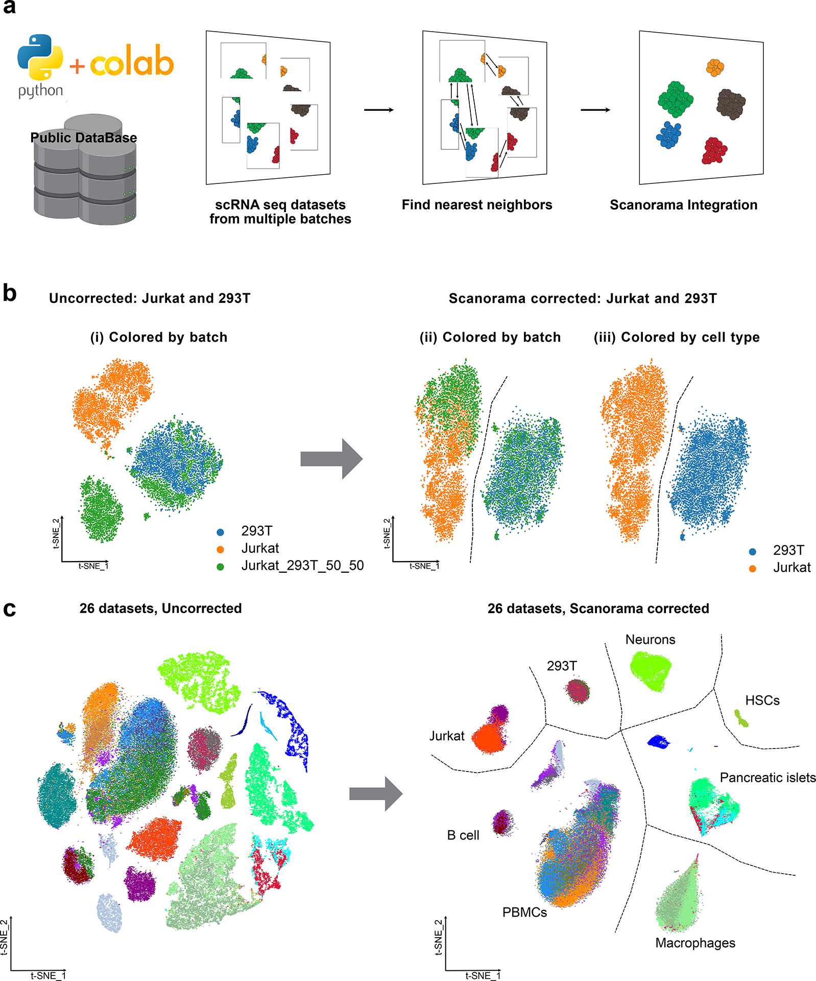
a, Integrating multiple single-cell RNA sequencing (scRNA-seq) datasets in a Colaboratory Python environment. Input datasets can be from public sources or user data. Scanorama conducts integration and batch correction, identifying shared cell types among batches by searching for nearest neighbors and aligns them into a shared space. b, Small dataset example: three datasets consisting of Jurkat cells, 293T cells, and a mixed population of these two cell types were used as the inputs and visualized using t-distributed stochastic neighbor embedding (t-SNE) before and after Scanorama correction. (ii-iii) Scanorama was able to accurately distinguish between Jurkat cells and 293T cells, originating from different batches (indicated by orange, green and blue) as distinct clusters (indicated by orange and blue). c, Large dataset 1 example: the Scanorama-integrated 26 single-cell datasets from 9 different technologies are visualized using t-SNE and clustered by cell types.

Furthermore, we expanded our protocol to include larger datasets. We combined 26 scRNA-seq datasets from nine different technologies, totaling 105,476 cells and 5,216 common genes. These datasets were obtained from 11 different studies^24–35. Consistent with our previous findings¹¹, Scanorama effectively identified datasets with similar cell types and integrated them, enabling clustering by cell type rather than by experimental batch (Fig. 1c).

Importantly, by incorporating optional steps such as sketching (step 12), parameter adjustments (step 21), and benchmarking integration methods (step 22), along with a comprehensive integration quality assessment using scib-metrics³, we observed that batch correction remained robust even up to a sketch size of 2500 cells (Supp. Fig 1). Adjustments in knn, sigma, and dimred parameters within the Scanorama integration process, outlined in our optional Step 21 and Supp. Fig 2, improved integration metrics related to biological conservation (KMeans NMI, KMeans ARI, Silhouette labels) without compromising batch correction efficacy (Silhouette batch, kBET metrics). This approach allowed us to determine parameters that balance noise reduction with the preservation of biological signal.

We also compare Scanorama to alternative methods for single-cell integration and show that Scanorama has competitive performance. The performance of Scanorama against the clustering-based model Harmony and deep learning-based integration approaches, scANVI and scVI showed that method performance varied based on integration task complexity. In agreement with original report by Luecken et al., we also found that Harmony performed well in simple tasks (Small dataset 1) but poorly in complex tasks (Large dataset 1). Conversely, Scanorama, scANVI, and scVI excelled in complex integration tasks (Supp. Fig 3).

Finally, we demonstrated the scalability of Scanorama using the Tabula Sapiens datasets, which represented three different organs and two different sequencing technologies. This dataset encompassed a total of 101,124 cells and 58,870 genes from seven donors. By utilizing ‘organ_tissue’ as a batch key, Scanorama successfully merged common immune cell types across the three organs and enabled clustering by cell type rather than by experimental batch, donor, or sequencing method (Fig. 2a–d). We can quantify this result by showing that the mutual information between labels obtained by unsupervised clustering on the integrated data and cell type labels (obtained by analyzing each tissue individually) is much higher than for labels corresponding to batch, donor, or method (Fig. 2e). In summary, this protocol demonstrates the robustness and scalability of Scanorama in integrating and analyzing scRNA-seq datasets, highlighting its ability to identify and merge similar cell types across different experimental conditions or technologies.

Figure 2. Panoramic integration of three organ single-cell datasets across seven donors and two different technologies.

a–d, The scRNA-seq datasets of three organs (a), seven donors (b), and two different technologies (c) from Tabula Sapiens were visualized using uniform manifold approximation and projection (UMAP), both before and after Scanorama correction. Cell clusters were grouped by cell type instead of batch factors such as organ, donor, and methods (d). e, Mutual information score between Leiden cluster labels and metadata (organ, donor, method, and cell types) after Scanorama correction.

Key points:

• Scanorama is an effective tool for combining multiple scRNA-seq datasets, addressing technical variation introduced by differences in sample preparation, sequencing depth, and experimental batches that can confound the analysis diverse datasets.

• Scanorama can handle multiple batches and dataset types while efficiently and accurately removing batch effects and identifying biologically relevant differences across datasets, making it a compelling option for scRNA-seq data integration.

Data Availability

The example datasets analyzed in this protocol are available from two repositories: Small and large dataset 1 is available from: https://zenodo.org/record/7968485/files; Large dataset 2 is available from: https://figshare.com/articles/dataset/Tabula_Sapiens_release_1_0/14267219.

References

- 1.Tabula Sapiens, C. et al. The Tabula Sapiens: A multiple-organ, single-cell transcriptomic atlas of humans. Science 376, eabl4896 (2022). [DOI] [PMC free article] [PubMed] [Google Scholar]
- 2.Eraslan G et al. Single-nucleus cross-tissue molecular reference maps toward understanding disease gene function. Science 376, eabl4290 (2022). [DOI] [PMC free article] [PubMed] [Google Scholar]
- 3.Luecken MD et al. Benchmarking atlas-level data integration in single-cell genomics. Nat Methods 19, 41–50 (2022). [DOI] [PMC free article] [PubMed] [Google Scholar]
- 4.Haghverdi L, Lun ATL, Morgan MD & Marioni JC Batch effects in single-cell RNA-sequencing data are corrected by matching mutual nearest neighbors. Nat Biotechnol 36, 421–427 (2018). [DOI] [PMC free article] [PubMed] [Google Scholar]
- 5.Butler A, Hoffman P, Smibert P, Papalexi E & Satija R Integrating single-cell transcriptomic data across different conditions, technologies, and species. Nat Biotechnol 36, 411–420 (2018). [DOI] [PMC free article] [PubMed] [Google Scholar]
- 6.Stuart T et al. Comprehensive Integration of Single-Cell Data. Cell 177, 1888–1902 e1821 (2019). [DOI] [PMC free article] [PubMed] [Google Scholar]
- 7.Korsunsky I et al. Fast, sensitive and accurate integration of single-cell data with Harmony. Nat Methods 16, 1289–1296 (2019). [DOI] [PMC free article] [PubMed] [Google Scholar]
- 8.Polanski K et al. BBKNN: fast batch alignment of single cell transcriptomes. Bioinformatics 36, 964–965 (2020). [DOI] [PMC free article] [PubMed] [Google Scholar]
- 9.Lopez R, Regier J, Cole MB, Jordan MI & Yosef N Deep generative modeling for single-cell transcriptomics. Nat Methods 15, 1053–1058 (2018). [DOI] [PMC free article] [PubMed] [Google Scholar]
- 10.Xu C et al. Probabilistic harmonization and annotation of single-cell transcriptomics data with deep generative models. Mol Syst Biol 17, e9620 (2021). [DOI] [PMC free article] [PubMed] [Google Scholar]
- 11.Hie B, Bryson B & Berger B Efficient integration of heterogeneous single-cell transcriptomes using Scanorama. Nat Biotechnol 37, 685–691 (2019). [DOI] [PMC free article] [PubMed] [Google Scholar]
- 12.Yu X, Xu X, Zhang J & Li X Batch alignment of single-cell transcriptomics data using deep metric learning. Nat Commun 14, 960 (2023). [DOI] [PMC free article] [PubMed] [Google Scholar]
- 13.Hie B, Cho H, DeMeo B, Bryson B & Berger B Geometric sketching compactly summarizes the single-cell transcriptomic landscape. Cell Syst 8, 483–493 e487 (2019). [DOI] [PMC free article] [PubMed] [Google Scholar]
- 14.Johnson WE, Li C & Rabinovic A Adjusting batch effects in microarray expression data using empirical Bayes methods. Biostatistics 8, 118–127 (2007). [DOI] [PubMed] [Google Scholar]
- 15.Lotfollahi M, Wolf FA & Theis FJ scGen predicts single-cell perturbation responses. Nat Methods 16, 715–721 (2019). [DOI] [PubMed] [Google Scholar]
- 16.Dasgupta S & Freund Y Random projection trees and low dimensional manifolds. Proceedings of the Annual ACM Symposium on Theory of Computing (2008). [Google Scholar]
- 17.Tran HTN et al. A benchmark of batch-effect correction methods for single-cell RNA sequencing data. Genome Biol 21, 12 (2020). [DOI] [PMC free article] [PubMed] [Google Scholar]
- 18.Buttner M, Miao Z, Wolf FA, Teichmann SA & Theis FJ A test metric for assessing single-cell RNA-seq batch correction. Nat Methods 16, 43–49 (2019). [DOI] [PubMed] [Google Scholar]
- 19.Halko N, Martinsson P-G & Tropp JA arXiv:0909.4061 (2009).
- 20.Yu YW, Daniels NM, Danko DC & Berger B Entropy-scaling search of massive biological data. Cell Syst 1, 130–140 (2015). [DOI] [PMC free article] [PubMed] [Google Scholar]
- 21.Wolf FA, Angerer P & Theis FJ SCANPY: large-scale single-cell gene expression data analysis. Genome Biol 19, 15 (2018). [DOI] [PMC free article] [PubMed] [Google Scholar]
- 22.Harris CR et al. Array programming with NumPy. Nature 585, 357–362 (2020). [DOI] [PMC free article] [PubMed] [Google Scholar]
- 23.Virshup I, Rybakov S, Theis FJ, Angerer P & Wolf FA anndata: Annotated data. bioRxiv, 2021.2012.2016.473007 (2021). [Google Scholar]
- 24.Zheng GX et al. Massively parallel digital transcriptional profiling of single cells. Nat Commun 8, 14049 (2017). [DOI] [PMC free article] [PubMed] [Google Scholar]
- 25.Gierahn TM et al. Seq-Well: portable, low-cost RNA sequencing of single cells at high throughput. Nat Methods 14, 395–398 (2017). [DOI] [PMC free article] [PubMed] [Google Scholar]
- 26.Paul F et al. Transcriptional Heterogeneity and Lineage Commitment in Myeloid Progenitors. Cell 163, 1663–1677 (2015). [DOI] [PubMed] [Google Scholar]
- 27.Nestorowa S et al. A single-cell resolution map of mouse hematopoietic stem and progenitor cell differentiation. Blood 128, e20–31 (2016). [DOI] [PMC free article] [PubMed] [Google Scholar]
- 28.Baron M et al. A Single-Cell Transcriptomic Map of the Human and Mouse Pancreas Reveals Inter- and Intra-cell Population Structure. Cell Syst 3, 346–360 e344 (2016). [DOI] [PMC free article] [PubMed] [Google Scholar]
- 29.Muraro MJ et al. A Single-Cell Transcriptome Atlas of the Human Pancreas. Cell Syst 3, 385–394 e383 (2016). [DOI] [PMC free article] [PubMed] [Google Scholar]
- 30.Grun D et al. De Novo Prediction of Stem Cell Identity using Single-Cell Transcriptome Data. Cell Stem Cell 19, 266–277 (2016). [DOI] [PMC free article] [PubMed] [Google Scholar]
- 31.Lawlor N et al. Single-cell transcriptomes identify human islet cell signatures and reveal cell-type-specific expression changes in type 2 diabetes. Genome Res 27, 208–222 (2017). [DOI] [PMC free article] [PubMed] [Google Scholar]
- 32.Segerstolpe A et al. Single-Cell Transcriptome Profiling of Human Pancreatic Islets in Health and Type 2 Diabetes. Cell Metab 24, 593–607 (2016). [DOI] [PMC free article] [PubMed] [Google Scholar]
- 33.Shalek AK et al. Single-cell RNA-seq reveals dynamic paracrine control of cellular variation. Nature 510, 363–369 (2014). [DOI] [PMC free article] [PubMed] [Google Scholar]
- 34.Davie K et al. A Single-Cell Transcriptome Atlas of the Aging Drosophila Brain. Cell 174, 982–998 e920 (2018). [DOI] [PMC free article] [PubMed] [Google Scholar]
- 35.Kang HM et al. Multiplexed droplet single-cell RNA-sequencing using natural genetic variation. Nat Biotechnol 36, 89–94 (2018). [DOI] [PMC free article] [PubMed] [Google Scholar]
- 36.DeMeo B & Berger B Recovering Single-cell Heterogeneity Through Information-based Dimensionality Reduction. bioRxiv, 2021.2001.2019.427303 (2022). [DOI] [PMC free article] [PubMed] [Google Scholar]
Associated Data
This section collects any data citations, data availability statements, or supplementary materials included in this article.
Supplementary Materials
Data Availability Statement