Abstract
To address rotor imbalance and misalignment in oil transfer pumps, an innovative diagnostic framework using Residual Network (ResNet) is proposed. The model incorporates advanced signal processing algorithms and strategic sensor placement to enhance diagnostic efficacy. A fault simulation test rig captured vibration signals from eight key measurement points on the pump. One-dimensional and multi-dimensional signal processing techniques generated comprehensive datasets for training and validating the model. Sensor placement optimization, focusing on the bearing seat's axial direction, inlet flange's vertical direction, and outlet flange's axial direction, increased rotor fault sensitivity. Time-frequency data processed via Short-Time Fourier Transform (STFT) achieved the highest diagnostic accuracy, surpassing 98 %. This study highlights the importance of optimal signal processing and precise sensor placement in improving the accuracy of diagnosing rotor faults in oil transfer pumps, thus enhancing the operational reliability and efficiency of energy transportation systems.
Keywords: Oil transfer pump, Rotor fault diagnosis, Residual networks (ResNet), Vibration analysis, Time-frequency analysis
Highlights
-
•
Combines Residual Networks (ResNet) with advanced signal processing for enhanced fault detection accuracy.
-
•
Employs strategic sensor placement for optimal sensitivity in detecting rotor imbalances and misalignments.
-
•
Achieves high diagnostic accuracies exceeding 98 % using Short-Time Fourier Transform (STFT).
-
•
Develops a comprehensive diagnostic framework tailored to the specific complexities of rotor faults in oil transfer pumps.
-
•
Advances fault diagnosis in energy systems, contributing to more reliable and efficient infrastructure maintenance.
1. Introduction
Oil transfer pumps are of paramount importance for the stability and efficiency of energy systems, significantly contributing to energy management and sustainability. These pumps facilitate the flow of oil through pipelines, which constitute a vital component of the global energy infrastructure, supporting a range of industrial and domestic needs. Efficient operation is of paramount importance in order to minimize energy loss and ensure the sustainable use of resources. Faults such as rotor imbalances and misalignments can have a significant impact on the operational stability and efficiency of these pumps, which in turn can affect energy conservation and the environmental footprint of energy production [[1], [2], [3], [4]]. Consequently, it is imperative to develop an efficacious fault diagnosis model for oil transfer pump rotors [5,6].
The prevailing approach to fault diagnosis is based on time-domain and frequency-domain analyses, including the Fourier Transform (FT) and the Hilbert Transform (HT). These methods identify the specific fault types by analyzing the spectral characteristics of the vibration signals. In the field of rotor fault diagnosis, traditional methods have been the subject of extensive research. Appana et al. [7] achieved a high diagnostic accuracy of 94.8 % by combining HT and FT with a one-dimensional convolutional neural network (1D-CNN). Shi et al. [8] put forth a dimensionality reduction algorithm that integrates time, frequency, and time-frequency domain characteristics for the purpose of rotor fault diagnosis. Almounajjed et al. [9] employed the discrete wavelet transform (DWT) to analyze current signals and proposed a novel fault estimation methodology based on mathematical equations and statistical parameters. However, these methods have limitations in their ability to handle complex and nonlinear signals, which can make it challenging to achieve high diagnostic accuracy.
In order to overcome the limitations of traditional methods, the researchers introduced machine learning techniques. These methods have demonstrated efficacy in categorizing fault types through the identification of patterns within the data. For example, Toma et al. [10] employed genetic algorithms and machine learning classifiers, including KNN, decision trees, and random forests, in their study, thereby demonstrating the efficacy and precision of these methods in fault diagnosis. Nevertheless, the application of machine learning methods is contingent upon the manual extraction of features, which is inherently challenging in the context of complex and variable fault signals [11].
In recent years, there has been a notable increase in the utilisation of deep learning techniques in the domain of fault diagnosis. The application of deep learning models enables the automatic extraction and learning of features from data, obviating the necessity for manual feature extraction. This significantly enhances the accuracy of fault diagnosis. For example, Miao et al. [12] enhanced an RNN, achieving superior accuracy and real-time capabilities compared to conventional approaches in diagnosing gearbox faults. Liu et al. [13] enhanced the robustness of their method by integrating LSTM with statistical analysis. Furthermore, Zhang et al. [14] employed a convolutional neural network (CNN) for feature extraction and subsequently integrated these features with a support vector machine (SVM), resulting in a model that demonstrated superior recognition rates during comparative evaluations. However, as the depth of the network increases, deep learning models encounter two significant challenges: gradient vanishing and gradient explosion. These challenges limit the potential for further performance improvement. To address these challenges, the Residual Network (ResNet) was developed.
The Residual Network (ResNet) represents an effective solution to the problem of gradient vanishing in the context of deep neural network training. The introduction of residual blocks to the ResNet model has resulted in enhanced training efficiency and feature extraction capabilities while maintaining the depth of the model. Hong et al. [15] employed a combination of ResNet and a Deep Collaborative Algorithm (DCA) to analyze fault characteristics in infrared images and vibration signals, thereby significantly enhancing diagnostic precision. In recent years, ResNet has been employed extensively in the domain of fault diagnosis, wherein it has been shown to offer substantial benefits in the context of intricate signal processing and the classification of faults with high precision. Ma et al. [16] combined various deep neural networks, including Deep Belief Networks, Convolutional Residual Networks, and Deep Self-Encoders, using a multi-objective optimization approach to enhance both accuracy and the ability to generalize in fault diagnosis tasks. Similarly, Guo et al. [17] introduced an attention-based ConvNeXt model with a parallel multistage dilated convolution residual module for the purpose of improving fault diagnosis in rotating machinery under noisy conditions. He et al. [18] introduced MFAN, a deep multi-signal fusion adversarial model, enhancing fault diagnosis in axial piston pumps via transfer learning and residual networks. Hou et al. [19] proposed a novel bearing fault diagnosis method using joint feature extraction of Transformer and ResNet, improving accuracy under noisy conditions and multiple working scenarios. While deep learning methods have gained traction in fault diagnosis research, studies specifically focusing on oil transfer pump rotor faults remain limited.
This paper presents a ResNet-based deep learning model for fault diagnosis of oil rotor pumps. Its development was inspired by the shortcomings of existing methods and by insights gained from other literatures. First, a fault simulation experimental device was designed to collect vibration signals at key measurement points of the oil rotor pump using high-precision vibration acceleration sensors and advanced signal processing techniques, such as short-time Fourier transform (STFT) and continuous wavelet transform (CWT). These techniques were applied to analyze the collected signals in the time-frequency domain and to extract key features. Subsequently, 1D and 2D ResNet models were constructed to automatically learn and extract complex features from the data through an end-to-end deep learning architecture, with the objective of achieving efficient and accurate fault classification. Furthermore, the application effects of various signal processing techniques on data from different measurement points were evaluated, with the aim of determining the sensitivity of different sensor layouts for fault detection.
The following section provides a comprehensive account of the experimental bench and sensor configuration utilized in this study. The third section will proceed with a comprehensive examination of the structure and functionality of the adopted network model. The fourth section will present a detailed demonstration of the performance of the method in a variety of experimental scenarios, with particular emphasis on the advantages of its application to the oil rotor pump test bed. In the final section, the primary findings and conclusions of this study will be presented in summary.
2. Simulation experiments and diagnostic strategy for oil transfer pump rotor faults
2.1. Experimental setup for rotor fault simulation
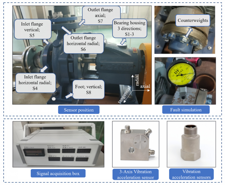
In this study, a single-machine, single-suction horizontal centrifugal pump of model AIX32/16 is employed as the test apparatus. Its principal technical parameters include the following: rated flow rate , rated speed , rated head , and specific rotation speed . To guarantee the precision of the experiment, the test apparatus has been constructed with a rubber flexible connector at the inlet and outlet flanges of the pump, which effectively eliminates the impact of piping vibration on the test data. The configuration of the oil transfer pump test set is illustrated in Fig. 1, and the principal components and performance indicators are listed in Table 1.
Fig. 1.
Experimental setup and sensor configuration for fault diagnosis of oil rotor pumps.
Table 1.
Principal components and their performance indicators.
| Name | Model Performance | Parameters |
|---|---|---|
| Signal acquisition box | Self-developed | High-frequency single-channel acquisition frequency: 10-200 k/s |
| Three-axis vibration 3211 acceleration sensor | Shanghai Le Zhen LZDY3 | Sensitivity:16 mA/g, error range:± 1 %, frequency range:1–10000 Hz |
| vibration acceleration sensor | Shanghai Le Zhen LZDY1 | Sensitivity: 100mv/g, error range:± 1 %, frequency range: 0.4–13000 Hz |
The pump unit is constructed on a robust cast iron base and is fixed to the pump body with a rigid connection. Furthermore, rubber shock-absorbing pads are strategically positioned between the base and the ground in order to effectively mitigate the effects of environmental variables on the testing process. In order to record the vibration characteristics of the oil transfer pump during a rotor fault, a total of eight measurement points are set up throughout critical areas of the pump. The aforementioned locations include the bearing housing, inlet flange, outlet flange, and the pump's feet. At these locations, high-precision vibration acceleration sensors have been installed for the purpose of collecting high-frequency vibration acceleration signals under various rotor fault conditions. The particular configuration of the sensors at each measurement point is delineated in Table 2.
Table 2.
Details of sensor placement.
| Types of sensors | Test Point | Position number |
|---|---|---|
| Three-axis vibration accelerometer | Bearing housing X-direction | S1 |
| Bearing housing Y-direction | S2 | |
| Bearing housing Z-direction | S3 | |
| Uniaxial vibration accelerometer | Imported flange Y-direction | S4 |
| Uniaxial vibration accelerometer | Imported flange Z-direction | S5 |
| Uniaxial vibration accelerometer | Export flange X-direction | S6 |
| Uniaxial vibration accelerometer | Export flange Y-direction | S7 |
| Uniaxial vibration accelerometer | Z-direction of the motor base | S8 |
Note:The X direction is defined as the axial direction, the Y direction as the horizontal radial direction, and the Z direction as the vertical direction.
2.2. Rotor fault simulation techniques
2.2.1. Simulating rotor unbalance faults
The objective of this experiment is to simulate an unbalanced rotor fault in an oil transfer pump. The specific weights of the load blocks are added to the coupling located at the non-driven end of the pump. The procedure entailed affixing the load block to the coupling and securely tightening the coupling bolts to guarantee that the load block remained stable throughout the operational cycle of the pump. This procedure resulted in an imbalance of the rotor system. In order to assess the impact of varying degrees of imbalance, three distinct weight categories of load blocks were selected: The weights in question were 3 g, 6 g, and 9 g, respectively. Following the introduction of each additional load, the vibration behaviour of the pump was meticulously documented with a view to analysing the impact of the failure. The process and precise location of the unbalanced loads are illustrated in Fig. 2.
Fig. 2.
Simulation of pump rotor unbalance fault.
2.2.2. Simulating rotor misalignment faults
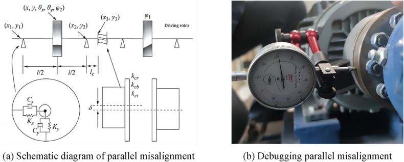
In the Rotor Misalignment Failure Simulation Experiment, a parallel misalignment of a pump shaft system was induced by precisely adjusting the motor shaft's horizontal position, thereby creating a parallel misalignment of the pump shaft system. This procedure was undertaken to simulate misalignments that might occur in a real-world operational context, due to factors such as installation errors or the wear and tear of the equipment. The displacements caused by the misalignment were set to 300 μm, 400 μm, and 500 μm, with the objective of studying and evaluating the specific effects of the shaft misalignment on the performance of the oil transfer pump. The experimental procedure is illustrated in Fig. 3.
Fig. 3.
Simulation of pump rotor parallel misalignment fault.
2.2.3. Detailed design of experimental protocols for rotor fault simulations
In order to gain insight into the vibration behavior of oil transfer pumps under rotor unbalance and misalignment faults, a series of experiments were conducted under varying rotational speeds and flow conditions. A frequency converter was employed to meticulously regulate the motor speed, enabling the experimentally determined speed ratios to be varied within the range of (where represents the actual set speed and is the rated speed). At the same time, the oil transfer pump operating flow rate ratio was set in the interval ( is the set operating flow rate and is the rated flow rate).
In order to ensure the comprehensiveness of the data, four separate sets of tests were conducted for each designated operating speed condition, with different flow rates. A total of 12 sets of tests were conducted under normal operating conditions. A total of 36 sets of tests were conducted under fault conditions of rotor unbalance and misalignment, forming a comprehensive test matrix with the objective of accurately depicting the vibration characteristics under these fault conditions.
In the initial phase of the test operation, the direct current (DC) inverter motor was brought to a preset speed by adjusting the frequency converter. Subsequently, the flow rate was meticulously regulated to the established level by adjusting the pump outlet valve. Once the oil transfer pump has reached a stable operating state, the vibration acceleration signals of each measurement point are collected in unison. In order to satisfy Nyquist's sampling law and to ensure signal integrity, the test sampling frequency was set at 25600 Hz, and the continuous sampling time for each group of tests was 1 s. The comprehensive test program for diverse fault types is presented in Table 3.
Table 3.
Test scheme for rotor failure simulation.
| Scheme number | Device status category | Fault simulation variation parameters | Experimental operating conditions |
|
|---|---|---|---|---|
| Rotational Speed (r/min) | Flow (m3/h) | |||
| 1–12 | Normal | None | 0.7n(2030r/min), 0.85n(2465 r/min), 1.0n(2900 r/min) |
0.7Qd(5.19 m3/h), 0.85Qd(6.31 m3/h), 1.0Qd(7.42 m3/h), 1.2Qd(8.90 m3/h) |
| 13–48 | rotor unbalance | 3 g | ||
| 6 g | ||||
| 9 g | ||||
| 49–84 | rotor misalignment | 300 μm | ||
| 400 μm | ||||
| 500 μm | ||||
3. Diagnostic methods for malfunctions
3.1. Enhancing data with Overlapping Sampling
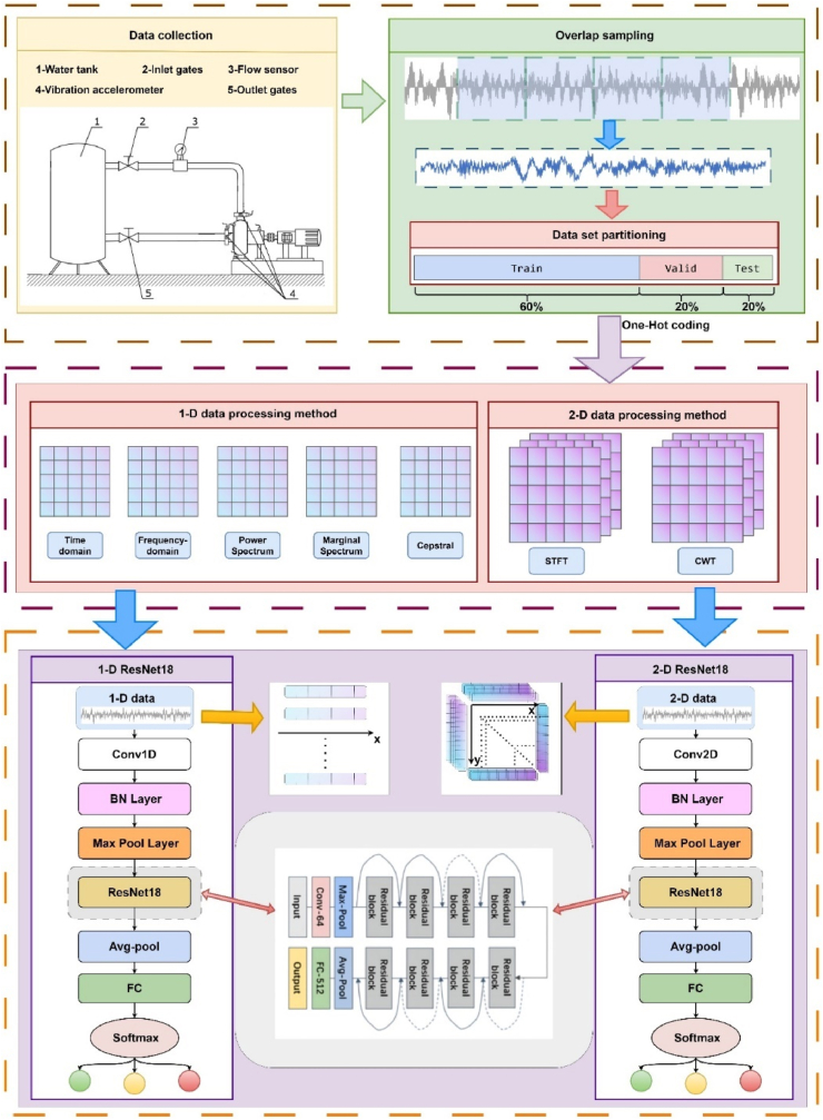
In this study, we use overlapping sampling to expand the data set, significantly increasing the number of samples while preserving temporal order and periodicity [20]. As shown in Fig. 4, this technique involves a sliding window that is moved stepwise over the original time-domain signal, where the window length determines the size of the new samples and the step size defines the interval between adjacent samples. The data are then partitioned, one-hot encoded, and processed using various 1D and 2D methods before being fed into the 1D-ResNet18 and 2D-ResNet18 models for training and evaluation.
Fig. 4.
Data collection and processing pipeline for 1D and 2D ResNet18 models.
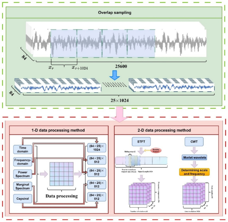
In the specific operation, we processed the 84 test data collected from each measurement point, each time with a data length of 25600 (including 12 normal operations and 36 unbalance and 36 misalignment state data). The overlapping sampling process is performed, and a window with a length of 1024 was also selected with a step size of 1024. The original signal was equally divided into a fault signal set consisting of 84 × 25 × 1024, which is a set of fault signals. The original signal is equally divided into an error signal set consisting of 84 × 25 × 1024.
To label the defect types, we adopted the one-hot coding strategy commonly used in multi-classification tasks and randomly partitioned the dataset into a training set (60 %), a test set (20 %), and a validation set (20 %). It is important to note that the segmentation was performed based on the total amount of data and not for each defect category, so the final proportion of each defect type in the dataset is not fixed [21].
3.2. Advanced signal processing for rotor fault analysis
In this study, we use overlapping sampling to expand the data set, significantly increasing the number of samples while preserving temporal order and periodicity. As shown in Fig. 5, in this technique, a sliding window is moved stepwise over the original time-domain signal, where the window length determines the size of the new samples and the step size defines the interval between adjacent samples. The data is then partitioned, one-hot encoded, and processed using various 1D (time domain, frequency domain, power spectrum, marginal spectrum, cepstral) and 2D (short-time Fourier transform, wavelet transform) methods before being fed into the respective models for training and evaluation.
Fig. 5.
Overlap sampling and data processing methods for 1D and 2D analysis.
3.2.1. 1-D signal analysis methods
-
(1)
Frequency Domain Analysis
The Fourier Transform (FT) serves as a cornerstone of signal analysis by converting time-domain signals into their frequency-domain counterparts, revealing the constituent frequency components. The Fast Fourier Transform (FFT) method is a common implementation where time domain data of length (1024, 1) is converted to frequency domain data of size (512, 1) by FFT. Mathematically, the FT is defined as follows:
| (1) |
where denotes the frequency spectrum of the signal .
-
(2)
Power Spectral Analysis
Power Spectral Density (PSD) analysis quantifies the power distribution across frequencies within a signal [22]. The PSD is defined by the following expression:
| (2) |
where is the PSD and is the Fourier Transform of the signal segment. In rotor fault diagnostics, examining peaks and patterns within the power spectrum can identify vibrational characteristics indicative of potential faults.
-
(3)
Marginal Spectrum Analysis
Marginal Spectrum Analysis, derived from the Hilbert-Huang Transform (HHT), is employed to capture the instantaneous frequency variations of a signal [23]. The calculation of the marginal spectrum is articulated as:
| (3) |
where is the marginal spectrum and represents the time-frequency distribution. This analysis is adept at handling non-linear and non-stationary signals, crucial for unveiling the dynamics of rotor faults.
-
(4)
Cepstral Analysis
Cepstral analysis identifies and separates modulatory features within a signal by computing the inverse Fourier Transform of the logarithm of the signal's spectrum. The cepstrum is computed as:
| (4) |
Where is the cepstrum, and denote the Fourier Transform and inverse Fourier Transform, respectively.
-
(5)
Short-Time Fourier Transform (STFT)
STFT provides time-frequency characteristics of a signal by applying the Fourier Transform within short sliding windows, and is mathematically formulated as:
| (5) |
Where is the window function, represents the time shift, and the frequency variable. The window size is (512, 1), the window sliding step is 12, the window function selects the hann window function, and the time-domain data is STFT-varied to obtain the time-frequency data of size (256, 43). STFT is crucial for dynamic fault analysis as it can pinpoint the timing and frequency content associated with a fault occurrence [24].
-
(6)
Wavelet Transform
The Continuous Wavelet Transform (CWT) furnishes a multi-scale time-frequency analysis technique, allowing signal examination at varying frequency resolutions [25]. The Morlet basis function is chosen for the wavelet basis function, and the time domain data is transformed to obtain time-frequency data of size (1024, 85). The expression for CWT is:
| (6) |
Where is the wavelet function. CWT is particularly effective in capturing transient and local features within a signal, crucial for the identification and localization of sudden rotor faults.
The details of the fault datasets produced by various signal processing methods and their application effects in different fault diagnosis scenarios is shown in detail in Table 4.
Table 4.
Details of data processed by different signal processing methods.
| Device Status | Dataset Details |
||||||
|---|---|---|---|---|---|---|---|
| Time-domain | Frequency-domain | Power Spectrum | Marginal Spectrum | Cepstral | Short-time Fourier Transform | Wavelet Transform | |
| Normal | (12 × 25) × 1024 |
(12 × 25) × 512 |
(12 × 25) × 512 | (12 × 25) × 512 | (12 × 25) × 512 | (12 × 25) × (256 × 43) |
(12 × 25) × (1024 × 85) |
| Rotor Unbalance | (36 × 25) × 1024 |
(36 × 25) × 512 |
(36 × 25) × 512 | (36 × 25) × 512 | (36 × 25) × 512 | (36 × 25) × (256 × 43) |
(36 × 25) × (1024 × 85) |
| Rotor Misalignment | (36 × 25) × 1024 |
(36 × 25) × 512 |
(36 × 25) × 512 | (36 × 25) × 512 | (36 × 25) × 512 | (36 × 25) × (256 × 43) |
(36 × 25) × (1024 × 85) |
Note:Dataset Details A × B (A: Number of Samples, B: Data Size).
3.3. Deep learning framework for fault diagnosis
3.3.1. The convolutional neural network (CNN) model
Convolutional Neural Network (CNN) is one of the core structures of deep learning and is particularly good at automatically extracting hierarchical features from raw data. It has demonstrated excellent performance in areas such as image recognition, speech processing, and natural language processing [26]. CNN efficiently captures abstract features in data through layer-by-layer feature extraction to achieve high accuracy in a variety of classification and recognition tasks. Its core structure includes an input layer, a convolutional layer, a ReLU layer, a pooling layer, and a fully connected layer, and the combination of these layers forms a network system capable of deep feature learning [27,28].
3.3.2. Implementing the ResNet model for fault diagnosis
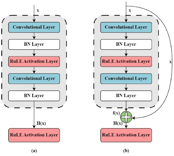
In deep neural networks, the increase of model depth is often accompanied by degradation phenomenon, i.e., the accuracy of the model will decrease with the increase of depth after reaching a certain stage. ResNet solves this problem by introducing shortcut connections [29]. Its core idea is to add direct mapping branches to form a Residual Block, whose mathematical model can be expressed as:
| (7) |
Where H(x) is the output, F(x) is the learning objective of the residual part, and x is the input of the residual block. When the residual part F(x) tends to 0, H(x) is directly equal to the input x. This ensures that the performance of the model is not degraded even if the depth of the network is increased [30].
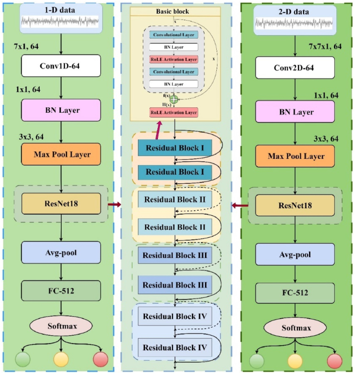
Residual structures in neural networks consist of multiple blocks, each containing an identity mapping and a residual component with convolutional layers, batch normalization layers, and activation functions. These blocks have shortcut connections that connect the input to the output of each residue block and channel into the activation function to produce the final output, as shown in Fig. 6. In addition, as shown in Fig. 7, the ResNet18 architecture consists of four residual structures, each containing two blocks. The architecture uses the initial layers for downsampling and the final layers for fully connected operations, resulting in a total of 18 layers. This design increases learning efficiency and output fidelity, making it suitable for various applications.
Fig. 6.
Comparison of convolutional residual block structures: (a) Standard convolutional block (b) residual convolutional block.
Fig. 7.
Overview of 1D and 2D ResNet18 architectures with residual blocks.
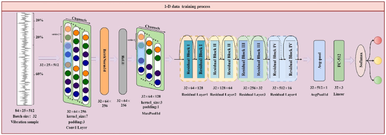
The 1D_ResNet architecture primarily consists of multiple Conv1d convolutional layers and Pool1d pooling layers, where the Conv1d kernel is adept at processing a variety of data types such as text, time series, spectral, and sentiment analysis [31]. As shown in Fig. 8, the architecture begins with initial convolution and pooling layers, followed by a series of residual blocks that improve feature extraction and learning efficiency. To provide a detailed understanding of the 1D ResNet architecture used in this study, Table 5 lists the specific hyperparameters and layer configurations used. Unlike the Conv2d kernel, which operates on two-dimensional spatial data primarily for image processing, the Conv1d kernel focuses on extracting features from one-dimensional data, making it ideal for analyzing sequences or signals. The Conv1d convolution operation is mathematically defined as:
| (8) |
Where represents the convolution output at time t, is the input signal at time , and denotes the convolution kernel weights at a shifted time . This operation effectively extracts features along the temporal or sequence axis of the data [32,33].
Fig. 8.
1D data training process with ResNet18 and residual blocks.
Table 5.
Hyperparameters and layer Configurations for 1D ResNet.
| Hyperparameter | Value |
|---|---|
| Input size | (32,25,512) |
| Batch size | 32 |
| Max epochs | 100 |
| Learning rate | 5e-5 |
| Optimizer | Adam |
| Conv1d | in_channels:25, out_channels:64,kernel_size:7,stride:2,padding:3 |
| BatchNorm1d | num_features: 64 |
| ReLU | – |
| MaxPool1d | kernel_size: 3, stride: 2, padding: 1 |
| BasicBlock Conv1d | in_channels: 64, out_channels: 64, kernel_size: 3, stride: 1, padding: 1 |
| Layer1 | output_channels: 64 |
| Layer2 | output_channels: 128, stride: 2 |
| Layer3 | output_channels: 256, stride: 2 |
| Layer4 | output_channels: 512, stride: 2 |
| AdaptiveAvgPool1d | output size: 1 |
| Linear | in_features: 512, out_features: 3 |
| Final output size | (32, 3) |
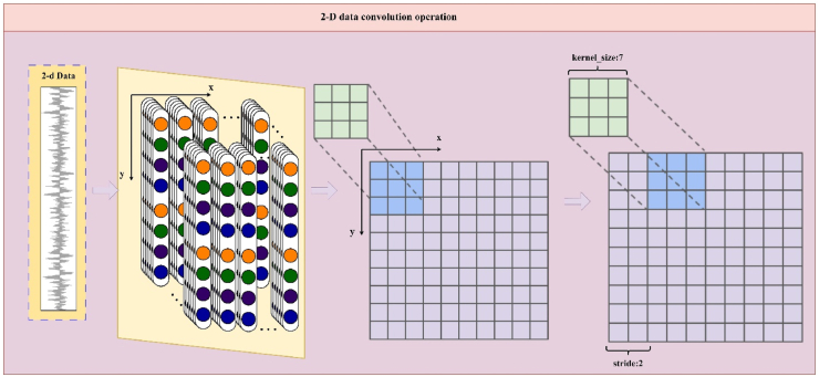
The 2D_ResNet architecture consists of several Conv2d convolutional layers and Pool2d pooling layers [34]. The Conv2d kernel is adept at extracting features from three-dimensional data by processing along two axes, which enhances the feature extraction capabilities. As shown in Fig. 9, the 2D convolution operation starts with a 2D input, and the kernel slides over the data in both the x- and y-directions, capturing spatial hierarchies. This process allows the model to learn complex patterns and relationships within the data, which is critical for image and spatial data analysis tasks. For a comprehensive overview of the 2D ResNet architecture, Table 6 lists the hyperparameters and layer configurations used in our experiments.
Fig. 9.
Convolution process for 2D data.
Table 6.
Hyperparameters and layer Configurations for 2D ResNet.
| Hyperparameter | Value |
|---|---|
| Input size | (32, 25, 256, 43) |
| Batch size | 32 |
| Max epochs | 100 |
| Learning rate | 5e-5 |
| Optimizer | Adam |
| Conv2d | in_channels:25, out_channels:64,kernel_size:7,stride:2,padding:3 |
| BatchNorm2d | num_features: 64 |
| ReLU | – |
| MaxPool2d | kernel_size: 3, stride: 2, padding: 1 |
| BasicBlock Conv2d | in_channels: 64, out_channels: 64, kernel_size: 3, stride: 1, padding: 1 |
| Layer1 | output_channels: 64 |
| Layer2 | output_channels: 128, stride: 2 |
| Layer3 | output_channels: 256, stride: 2 |
| Layer4 | output_channels: 512, stride: 2 |
| AdaptiveAvgPool2d | output size: 1 |
| Linear | in_features: 512, out_features: 3 |
| Final output size | (32, 3) |
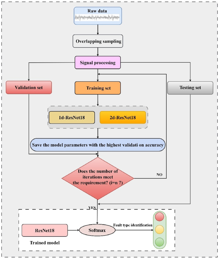
Following the oil transfer pump rotor fault simulation experiments, vibration acceleration signals were meticulously gathered at strategic measurement points across the pump under varying operational conditions. As depicted in Fig. 10, the flowchart elaborates on the methodology adopted for the rotor fault type diagnosis in the oil transfer pump, entailing the ensuing pivotal steps:
-
(1)
: Overlapping sampling of raw data from measurement points, followed by signal processing to generate a fault dataset.
-
(2)
: The fault dataset is split into fixed proportions of training, validation, and testing sets, and the model iteration number n is set.
-
(3)
: If the fault data is one-dimensional, the training set is fed into a 1D_ResNet18 model for training. If the fault data is two-dimensional, the training set is fed into a 2D_ResNet18 model for training. The iteration produces a trained model.
-
(4)
: After the validation set enters the iteration of the completed model, if the current validation accuracy is greater than the historical validation accuracy, the current model parameters are saved, and i is incremented by (i = i+1).
-
(5)
: If i < n, repeat step (3); if i = n, proceed to step (6).
-
(6)
: The saved model parameters from step (4) are loaded back into the ResNet18 model, and the testing set is fed into the model. The fault diagnosis result is obtained by passing the output through a SoftMax function.
Fig. 10.
Workflow of signal processing and model training using 1D and 2D ResNet18.
4. Fault diagnosis using time-domain and frequency-domain signals
4.1. Analysis of time-domain data for fault diagnosis
In the quest to diagnose oil transfer pump rotor faults with increased accuracy, the adoption of the Rectified Linear Unit (ReLU) function, the Cross Entropy Loss function, and the Adam optimization algorithm within the 1D_ResNet18 model framework results from a strategic alignment with principles that enhance model effectiveness and diagnostic accuracy.
The Cross Entropy loss function is employed for its aptness in classification endeavors, offering a quantitative measure of the disparity between the predicted probabilities and actual labels, thereby imposing stringent penalties on misclassifications to refine predictive performance iteratively. Mathematically, it's defined for a binary classification as:
| (9) |
Where is the true label, and is the predicted probability for the observation.
Accuracy, measures the proportion of correct predictions among the total number of cases are examined in the context of classification models. It serves as a straightforward metric for evaluating the model's performance, particularly in scenarios where the class distribution is relatively balanced [35]. To complement the Cross Entropy loss function's focus on probability disparities, accuracy is calculated as follows:
| (10) |
Where, is an indicator function that returns 1 if the predicted label for observation matches the true label , and 0 otherwise.
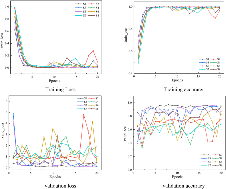
The variations in loss and diagnostic accuracy observed during the training and validation phases, as shown in Fig. 11, indicate that the training loss stabilizes after about four iterations for most measurement points. However, the validation phase showed significant fluctuations in both loss and accuracy for the time-domain data, suggesting that the models lack robustness when trained with data from most of the measurement points. Notably, measurement points S1 and S4 showed less volatility in validation loss and accuracy, indicating greater stability in model training. This variability is likely due to the different sensitivities of the measurement points to rotor imbalance and misalignment errors in oil transfer pumps. As a result, models trained with time-domain data from specific measurement points do not consistently capture features that reflect the operating condition of the oil transfer pump rotor, resulting in cyclic patterns of loss and noticeable fluctuations in accuracy during validation.
Fig. 11.
The loss and accuracy curves for training and validation of temporal domain data.
The t-SNE clustering method [36] is praised for its ability to deal with the dimensionality reduction of high-dimensional data and maintain the local structural characteristics of the data after dimensionality reduction, and its mathematical expression is as follows:
| (11) |
Where is the conditional probability in the high-dimensional space, and is the conditional probability in the dimensionality reduction space.
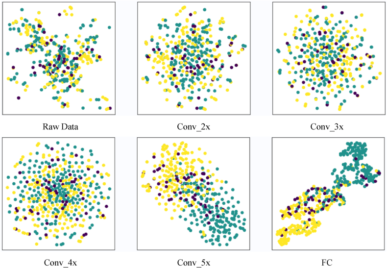
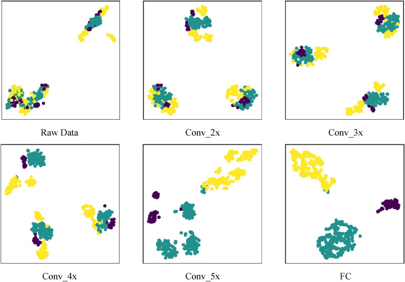
The goal was to thoroughly evaluate the distribution of the feature space data, as shown in Fig. 12. The analysis showed that the clustering properties of the time-domain data did not show significant improvement after processing through the deep network architecture. Even after the data passed through the final fully connected layer of the network, the feature articulation still failed to achieve satisfactory clustering results. The lack of clear separation between different equipment states, characterized by significant overlap and mixing of data points, severely compromises the accuracy of fault diagnosis for oil transfer pump rotors. This indicates a critical need for improved feature extraction techniques or model adjustments to increase diagnostic accuracy.
Fig. 12.
Feature clustering diagram of time-domain data at different stages in the model.
4.2. Frequency-domain data analysis for enhanced fault identification
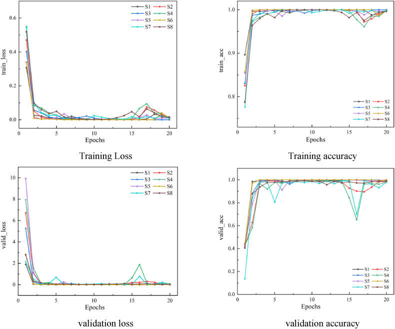
In this study, training and validation of a 1D_ResNet18 model were performed using frequency domain data collected from different measurement points, using the same model configurations as discussed in Section 4.1, including the activation function, loss function, and optimization algorithm. The training and validation loss trends, as well as the diagnostic accuracy across measurement points at each iteration, are shown in Fig. 13. In particular, Figs. 13.1 and 13.2 show that the losses and diagnostic accuracies for each measurement point began to stabilize after the first three iterations of the training process. The loss values remained consistently low throughout the training period, with only minor fluctuations at certain points, particularly around the 16th iteration. These fluctuations during the 16th iteration, observed in the diagnostic accuracy of both the training and validation sets (Figs. 13.3 and 13.4), are likely due to the behavior of the optimization algorithm as it searches for the global optimum of the model.
Fig. 13.
The variation curves of loss and accuracy during training and validation of frequency-domain data.
As shown in Fig. 14, the t-SNE dimensionality reduction and clustering technique using frequency domain data along with the features extracted from the four residual blocks and the fully connected layer of the network model provides insightful clustering maps. The first three residual blocks may not yield optimal clustering results; however, after the Conv_4× residual block, the clustering effectiveness significantly exceeds that observed with time-domain data. Despite some overlap between the normal operating state and the rotor imbalance fault within the Conv_4× block, the rotor imbalance fault is clearly separated from the other two states. Furthermore, after traversing the fully connected layer, the differentiation between the normal state and the rotor unbalance fault becomes more pronounced, demonstrating the ability of the network to refine and accentuate feature distinctions critical to accurate fault diagnosis.
Fig. 14.
Feature clustering graph of frequency-domain data at different stages in the model.
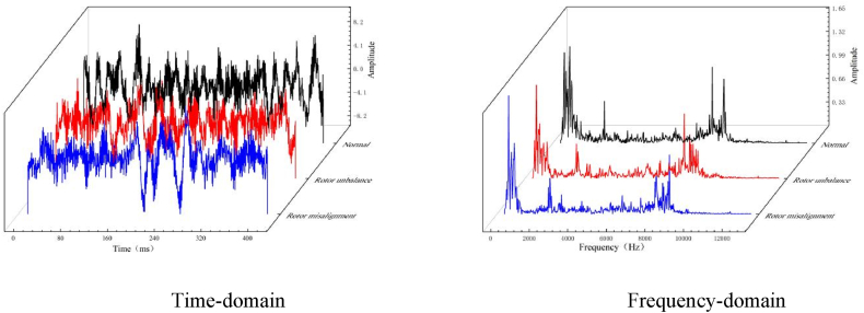
The previous analysis thoroughly evaluated the comparative performance of time-domain and frequency-domain data sets for diagnosing rotor faults in oil transfer pumps. The investigation revealed that frequency domain data provided superior diagnostic accuracy with reduced loss variation, especially in the validation data set. To illustrate, data segments representing various oil transfer pump rotor failures, all under a consistent operating condition (2900 rpm, 7.42 m3/h), were analyzed in both domains.
The analysis presented in Fig. 15 shows that the time domain data from the oil transfer pump under these conditions did not show clear patterns that could differentiate the operating state of the equipment. This complexity is due to the internal structural intricacies of the pump and its load state during operation. Conversely, the frequency domain representation revealed a predominant concentration of energy in both the low and high frequency regions, with a notable emphasis on the low frequency components. In this domain, rotor unbalance and misalignment faults were clearly marked by abnormal amplitude variations at lower harmonics, such as a significant amplitude spike at the first harmonic, indicative of rotor unbalance faults [37].
Fig. 15.
Comparison of Time-domain data and Frequency-domain data in different fault types.
Note: The blue line represents the fault of rotor misalignment, the red line represents the fault of rotor unbalance, and the black line represents the normal state. (For interpretation of the references to colour in this figure legend, the reader is referred to the Web version of this article.)
4.3. Comparative analysis of signal processing methods
The previous discussions highlight the varying effects of signal processing techniques on the accuracy of deep learning models in diagnosing oil transfer pump rotor faults. It's clear that frequency domain data significantly improves fault diagnosis compared to time domain data. Using datasets processed by the signal processing methods outlined earlier (as detailed in Table 4), this section will delve into a comparative analysis of how different signal processing methods influence diagnostic results at different measurement points for oil transfer pump rotor faults [38].
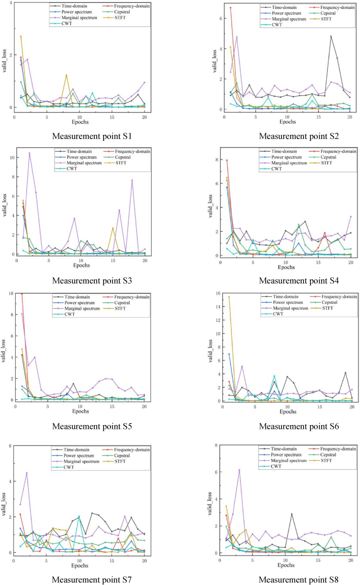
The analysis used 1D_ResNet18 network models for one-dimensional data and 2D_ResNet18 network models for two-dimensional data. Uniform initial parameters, activation functions, optimization algorithms, and loss functions were maintained across models prior to training. After 20 iterations, models trained with different signal processing methods were found to differ in robustness, as shown in Fig. 16. Specifically, models using frequency domain data, power spectral data, Short-Time Fourier Transform (STFT) data, and Continuous Wavelet Transform (CWT) data demonstrated superior stability, as evidenced by their low validation losses in the initial iterations. In contrast, models trained on marginal spectral and time-domain data exhibited oscillations and struggled to converge.
Fig. 16.
The curve of the loss of different measuring points validation-sets with the number of Epochs.
Differences in the validation losses at different measurement points further highlighted the performance of the models, with the S1 measurement point experiencing small validation loss fluctuations for certain signal processing techniques, but eventually converging. On the other hand, the S7 location consistently showed higher losses across models trained with different signal processing techniques. This discrepancy highlights the different sensitivities of the oil transfer pump points to rotor imbalance and misalignment errors. Although each measurement point collects information about the operating condition of the pump rotor, some may only capture partial information, which hampers the model's ability to extract key features indicative of rotor faults and consequently reduces the accuracy of fault diagnosis.
The diagnostic accuracy of rotor faults at different measurement points using different signal processing techniques is detailed in Table 7. These data show that models trained with frequency domain data, power spectral analysis, and STFT time-frequency spectra consistently outperform those trained with alternative signal processing techniques in terms of fault diagnostic accuracy. In particular, training with marginal spectrum data yields the least effective fault diagnosis, with the maximum diagnostic accuracy for any measurement point capped at 84.60 %. Among the various methods evaluated, the S1 measurement point (located at the bearing seat in the X-direction) proved to be the most accurate in fault diagnosis, indicating its increased sensitivity to fault conditions, while S8 recorded the lowest accuracy figures.
Table 7.
Comparison of test accuracy.
| Signal type | Diagnostic accuracy at different measuring points (%) |
|||||||
|---|---|---|---|---|---|---|---|---|
| Bearing seat |
Imported flange |
Exported flange |
Motor base |
|||||
| S1 | S2 | S3 | S4 | S5 | S6 | S7 | S8 | |
| Time- domain | 96.65 | 78.79 | 96.21 | 67.19 | 88.17 | 86.38 | 66.74 | 81.7 |
| Frequency-domain | 99.78 | 99.55 | 99.78 | 98.21 | 100 | 100 | 97.1 | 99.11 |
| Power spectrum | 99.55 | 97.99 | 99.11 | 98.88 | 100 | 100 | 95.09 | 98.44 |
| Cepstral | 98.66 | 91.74 | 98.66 | 83.93 | 98.66 | 97.32 | 85.94 | 87.05 |
| Marginal Spectrum | 89.51 | 67.86 | 87.05 | 56.92 | 84.60 | 68.08 | 75.45 | 69.20 |
| STFT | 100 | 99.33 | 99.33 | 99.33 | 100 | 99.33 | 99.78 | 98.44 |
| CWT | 97.45 | 99.54 | 99.77 | 96.06 | 99.31 | 99.77 | 99.77 | 98.15 |
This variability in diagnostic accuracy underscores the different sensitivity of sensors positioned in different orientations to fault conditions. For example, the S1 point demonstrates a superior ability to diagnose fault types than the S2 point (located at the bearing seat in the Y direction), due to the complex internal structure of the oil transfer pump. This complexity introduces redundant information into the collected signals, which is influenced by factors such as sensor placement and the vibration characteristics associated with different fault types, such as rotor imbalance or misalignment.
5. Conclusion
This study explored the diagnosis of rotor unbalance and misalignment faults in oil transfer pumps, by analyzing data collected from eight strategically positioned high-frequency vibration sensors. The major findings are as follows:
-
1.
Techniques such as frequency domain analysis, power spectrum analysis, Short-Time Fourier Transform (STFT), and wavelet transform were found to be highly effective in diagnosing pump rotor failures. In particular, the application of STFT resulted in diagnostic accuracies exceeding 98 %, highlighting the integration of sophisticated signal processing with machine learning as particularly beneficial.
-
2.
The research revealed significant variability in the sensitivity of different measurement points to faults, which significantly affected the quality and integrity of the data collected. The positioning of sensors at the axial bearing seat, vertical inlet flange, and axial outlet flange proved to be critical to obtaining accurate diagnostics.
-
3.
The research helped advance the application of signal processing and deep learning to the diagnosis of rotor faults in oil transfer pumps. These findings provide a foundation for future improvements in the diagnosis of rotating machinery faults, promoting more reliable and efficient power generation systems.
CRediT authorship contribution statement
Lei Chen: Investigation, Methodology, Resources, Writing – original draft. Liang Dong: Conceptualization, Investigation, Methodology, Validation, Writing – original draft. Zhi-Cai Wu: Conceptualization, Data curation, Methodology, Software. Chuan-Han Fan: Conceptualization, Data curation, Methodology, Supervision. Wei-Hua Shi: Funding acquisition, Methodology. Hong-Gang Li: Software, Validation. Ru-Nan Hua: Funding acquisition, Supervision. Cui Dai: Conceptualization, Funding acquisition, Project administration, Supervision.
Declaration of competing interest
The authors declare that they have no known competing financial interests or personal relationships that could have appeared to influence the work reported in this paper.
Acknowledgments
The authors would like to thank the financial support from National Natural Science Foundation of China (No. 52279087,51879122), Program Development of Jiangsu Higher Education Institutions (PAPD), and Jiangsu top six talent summit project (GDZB-017).
Contributor Information
Liang Dong, Email: dongliang@usj.edu.cn.
Cui Dai, Email: daicui@ujs.edu.cn.
References
- 1.Liu B., Xu C., Li G., Yang Y., Dai L.L. Application of frequency domain analysis method in vibration analysis and Fault Diagnosis of oil transfer pump unit. J. Phys. Conf. 2023;2437 [Google Scholar]
- 2.Dong L., Xiao Q., Jia Y., Fang T. Review of research on intelligent diagnosis of oil transfer pump malfunction. Petroleum. 2022;9(2):135–142. [Google Scholar]
- 3.Dong L., Chen Z., Hua R., Hu S., Fan C., Xiao X. Research on diagnosis method of centrifugal pump rotor faults based on IPSO-VMD and RVM. Nucl. Eng. Technol. 2022;55(3):827–838. [Google Scholar]
- 4.Wang L., Liu H., Liang J., Zhang L., Ji Q., Wang J. Research on the rotor Fault Diagnosis method based on QPSO-VMD-PCA-SVM. Front. Energy Res. 2022;2022 [Google Scholar]
- 5.Yang Zhaoming, Liu Zhe, Zhou Jing, Song Chaofan, Qi Xiang, He Qian, Hu Jingjing, Faber Michael H., Zio Enrico, Li Zhenlin, Su Huai, Zhang Jinjun. A graph neural network (GNN) method for assigning gas calorific values to natural gas pipeline networks. Energy. 2023;278 doi: 10.1016/j.energy.2023.127875. ISSN 0360-5442. [DOI] [Google Scholar]
- 6.Jiang Q., Bao B., Hou X., Huang A., Jiang J., Mao Z. Feature mining and sensitivity analysis with adaptive sparse attention for bearing Fault Diagnosis. Appl. Sci. 2023;13(2):718. [Google Scholar]
- 7.Appana D.K., Ahmad W., Kim J. Speed invariant bearing fault characterization using convolutional neural networks. International Workshop on Multi-disciplinary Trends in Artificial Intelligence. 2017;2017:189–198. [Google Scholar]
- 8.Shi M., Zhao R., Wu Y., et al. F ault diagnosis of rotor based on local-global balanced orthogonal discriminant projection. Measurement. 2021;168 [Google Scholar]
- 9.Almounajjed A., Sahoo A.K., Kumar M.K. Diagnosis of stator fault severity in induction motor based on discrete wavelet analysis. Measurement. 2021;182 [Google Scholar]
- 10.Toma R.N., Prosvirin A.E., Kim J. Bearing Fault diagnosis of induction motors using a genetic algorithm and machine learning classifiers. Sensors. 2020;20 doi: 10.3390/s20071884. Basel, Switzerland. [DOI] [PMC free article] [PubMed] [Google Scholar]
- 11.Fernandes M., Corchado J.M., Marreiros G. Machine learning techniques applied to mechanical fault diagnosis and fault prognosis in the context of real industrial manufacturing use-cases: a systematic literature review. Appl. Intell. 2022;52(12):14246–14280. doi: 10.1007/s10489-022-03344-3. [DOI] [PMC free article] [PubMed] [Google Scholar]
- 12.Miao X., Li S., Zhu Y., et al. A novel real-time Fault Diagnosis method for planetary gearbox using transferable hidden layer. IEEE Sensor. J. 2020;20(15):8403–8412. [Google Scholar]
- 13.Liu J., Pan C., Lei F., et al. Fault prediction of bearings based on LSTM and statistical process analysis. Reliab. Eng. Syst. Saf. 2021;214 [Google Scholar]
- 14.Zhang X., Han P., Xu L., et al. Research on bearing Fault Diagnosis of wind turbine gearbox based on 1DCNN-PSO-SVM. IEEE Access. 2020;8:192248–192258. [Google Scholar]
- 15.Hong X., Duan L., Zhang L. Multi-sensor heterogeneous data fusion method for rotor system diagnosis based on multi-mode residual network and discriminant correlation analysis. Meas. Sci. Technol. 2021;32 [Google Scholar]
- 16.Ma S., Chu F. Ensemble deep learning-based fault diagnosis of rotor bearing systems. Comput. Ind. 2019;105:143–152. [Google Scholar]
- 17.Guo B., Qiao Z., Zhang N., Wang Y., Wu F., Peng Q. Attention-based ConvNeXt with a parallel multiscale dilated convolution residual module for fault diagnosis of rotating machinery. Expert Syst. Appl. 2024;2024 [Google Scholar]
- 18.He Y., Tang H., Ren Y., Kumar A. A deep multi-signal fusion adversarial model based transfer learning and residual network for axial piston pump fault diagnosis. Measurement. 2022;192(2) [Google Scholar]
- 19.Hou S., Lian A., Chu Y. Bearing fault diagnosis method using the joint feature extraction of Transformer and ResNet. Meas. Sci. Technol. 2023;34 [Google Scholar]
- 20.Wang C., Zheng Z., Guo D., Liu T., Xie Y., Zhang D. An experimental Setup to detect the crack fault of asymmetric rotors based on a deep learning method. Appl. Sci. 2023;13(3):1327. [Google Scholar]
- 21.Dai C., Dong L., Zhang X., et al. Experimental and internal flow investigation on the performance of a hydraulic retarder with different liquid-filled amount and blade inclination angles. J. Therm. Sci. 2022;31:923–933. [Google Scholar]
- 22.Yi C., Wang H., Ran L., Zhou L., Lin J. Power spectral density-guided variational mode decomposition for the compound fault diagnosis of rolling bearings. Measurement. 2022 199.111494. [Google Scholar]
- 23.Wang H., Ji Y. A revised hilbert–huang transform and its application to Fault Diagnosis in a rotor system. Sensors. 2018;18(12):4329. doi: 10.3390/s18124329. [DOI] [PMC free article] [PubMed] [Google Scholar]
- 24.Tao H., Wang P., Chen Y., Stojanovic V., Yang H. An unsupervised fault diagnosis method for rolling bearing using STFT and generative neural networks. J. Franklin Inst. 2020;357:7286–7307. [Google Scholar]
- 25.Diao N., Wang Z., Ma H., et al. Fault diagnosis of rolling bearing under variable working conditions based on CWT and T-ResNet. J. Vib. Eng. Technol. 2023;11:3747–3757. [Google Scholar]
- 26.Wen L., Li X., Gao L., Zhang Y. A new convolutional neural network-based data-driven Fault Diagnosis method. IEEE Trans. Ind. Electron. 2018;65:5990–5998. [Google Scholar]
- 27.Chen X., Zhang B., Gao D. Bearing fault diagnosis base on multi-scale CNN and LSTM model. J. Intell. Manuf. 2021;32(4):971–987. [Google Scholar]
- 28.Dao Fang, Zeng Yun, Qian Jing. Fault diagnosis of hydro-turbine via the incorporation of bayesian algorithm optimized CNN-LSTM neural network. Energy. 2024;290(0360–5442) doi: 10.1016/j.energy.2024.130326. ISSN. [DOI] [Google Scholar]
- 29.He K., Zhang X., Ren S., Sun J. IEEE Conference on Computer Vision and Pattern Recognition (CVPR); 2015. Deep Residual Learning for Image Recognition. 2016; pp. 770–778. [Google Scholar]
- 30.Nutkiewicz A., Yang Zheng, Jain R.K. Data-driven Urban Energy Simulation (DUE-S): a framework for integrating engineering simulation and machine learning methods in a multi-scale urban energy modeling workflow. Appl. Energy. 2018;225:1176–1189. [Google Scholar]
- 31.Chen C., Liu Z., Yang G., Wu C., Ye Q. An improved Fault Diagnosis using 1D-convolutional neural network model. Electronics. 2020;10(1):59. [Google Scholar]
- 32.Jiang W., Wang C., Zou J., Zhang S. Application of deep learning in Fault Diagnosis of rotating machinery. Processes. 2021;9(6):919. [Google Scholar]
- 33.Wu C., Jiang P., Ding C., Feng F., Chen T. Intelligent fault diagnosis of rotating machinery based on one-dimensional convolutional neural network. Comput. Ind. 2019;108:53–61. [Google Scholar]
- 34.Wang J., Wang D., Wang S., Li W., Song K. Fault diagnosis of bearings based on multi-sensor information fusion and 2D convolutional neural network. IEEE Access. 2021;9:23717–23725. [Google Scholar]
- 35.Nath A.G., Sharma A., Udmale S.S., Singh S.K. An early classification approach for improving structural rotor Fault Diagnosis. IEEE Trans. Instrum. Meas. 2021;70:1–13. [Google Scholar]
- 36.Du W., Hu P., Wang H., Gong X., Wang S. Fault diagnosis of rotating machinery based on 1D–2D joint convolution neural network. IEEE Trans. Ind. Electron. 2023;70:5277–5285. [Google Scholar]
- 37.Marins M.A., Ribeiro F.M.L., Netto S.L., et al. Improved similarity-based modeling for the classification of rotating-machine failures. J. Franklin Inst. 2018;355(4):1913–1930. [Google Scholar]
- 38.Hu X., Wei D., Liu D., Xiao Z., Xia X., Malik O.P. Fault diagnosis for rotor based on multi-sensor information and progressive strategies. Meas. Sci. Technol. 2023;34 [Google Scholar]


