Salty chemical cocktails as water quality signatures: longitudinal trends and breakpoints along different U.S. streams

Abstract

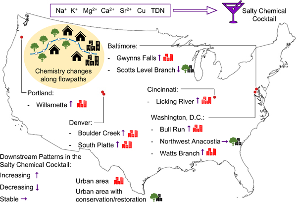
Along urban streams and rivers, various processes, including road salt application, sewage leaks, and weathering of the built environment, contribute to novel chemical cocktails made up of metals, salts, nutrients, and organic matter. In order to track the impacts of urbanization and management strategies on water quality, we conducted longitudinal stream synoptic (LSS) monitoring in nine watersheds in five major metropolitan areas of the U.S. During each LSS monitoring survey, 10–53 sites were sampled along the flowpath of streams as they flowed along rural to urban gradients. Results demonstrated that major ions derived from salts (Ca²⁺, Mg²⁺, Na⁺, and K⁺) and correlated elements (e.g. Sr²⁺, N, Cu) formed ‘salty chemical cocktails’ that increased along rural to urban flowpaths. Salty chemical cocktails explained 46.1% of the overall variability in geochemistry among streams and showed distinct typologies, trends, and transitions along flowpaths through metropolitan regions. Multiple linear regression predicted 62.9% of the variance in the salty chemical cocktails using the six following significant drivers (p<0.05): percent urban land, wastewater treatment plant discharge, mean annual precipitation, percent silicic residual material, percent volcanic material, and percent carbonate residual material. Mean annual precipitation and percent urban area were the most important in the regression, explaining 29.6% and 13.0% of the variance. Different pollution sources (wastewater, road salt, urban runoff) in streams were tracked downstream based on salty chemical cocktails. Streams flowing through stream-floodplain restoration projects and conservation areas with extensive riparian forest buffers did not show longitudinal increases in salty chemical cocktails, suggesting that there could be attenuation via conservation and restoration. Salinization represents a common urban water quality signature and longitudinal patterns of distinct chemical cocktails and ionic mixtures have the potential to track the sources, fate, and transport of different point and nonpoint pollution sources along streams across different regions.

Graphical Abstract

1. Introduction

Urbanization is impacting water quality on a global scale with risks due to point and nonpoint source pollution (Grimm et al., 2008; Kaushal et al., 2011; Paul and Meyer, 2001; Walsh et al., 2005). Various urban contaminants including nutrients (Dodds, 2007; Evans-White et al., 2013; Paul and Meyer, 2001), heavy metals (Farid et al., 2012), and microbes (Parr et al., 2016) are regulated. There are also many emerging contaminants of concern, which are less frequently regulated, including pharmaceuticals (Masoner et al., 2019; Peña-Guzmán et al., 2019) and salt pollution from road salts, sewage, and weathering of the urban environment (Bhide et al., 2021; Corsi et al., 2010; Kaushal et al., 2021, 2019, 2018b, 2017, 2005; Wright et al., 2011). Novel and distinct elemental combinations, known as chemical cocktails, are formed in urban watersheds due to shared sources, flowpaths, and biogeochemical interactions (Kaushal et al., 2020, 2018a). By measuring multiple chemical constituents and classifying them as chemical cocktails, we can holistically understand and co-manage groups of contaminants (Galella et al., 2021; Kaushal et al., 2023a, 2020; Morel et al., 2020). Here, we investigate whether there are common chemical cocktails formed as streams and rivers flow through different U.S. cities, reflecting typical urban sources and biogeochemical processes. We also investigate whether these chemical cocktails have the potential to be attenuated or reduced as streams flow through parks and restoration areas (Kaushal et al., 2022; Kaushal et al., 2023a, Maas et al., 2023). This work is intended to further our understanding of whether we can improve pollution source tracking approaches across watersheds by detecting longitudinal trends and transitions of pollutants along flowpaths.

There is specifically a need to conduct such research at a national scale, as exemplified here, in order to understand what urban contaminants and processes are generalizable across cities (Chambers et al., 2016; McPhearson et al., 2016). Previous work has examined how flood vulnerability (Chang et al., 2021), hydrological flow response (Hopkins et al., 2015a, 2015b), stormwater quality (Balderas Guzman et al., 2022), nitrogen (Brown et al., 2009), and organic pollutants (Bradley et al., 2021, 2019; Brown et al., 2009; Kolpin et al., 2002) are impacted by urbanization across cities. However, more work is needed to specifically identify the generalizable impacts of urbanization on inland freshwater salinization. For example, more work is needed to understand the relative role of how different state factors, such as climate, human activities (including land use and wastewater treatment plants), underlying geology, time, and flowpaths, alter salinization responses across different metropolitan regions (Kaushal et al. 2023b). In this paper, we use the terms “salt”, “salinity”, and “salt ions” to reference all major ions, which are often derived from salts, or ionic compounds (Kaushal et al., 2023c).

Salinity has been suggested as a universal signature of urbanization (Kaushal et al., 2014a), but most regional comparisons focus on specific conductance or only one major ion (Brown et al., 2009; Kaushal et al., 2018b; Moore et al., 2020). However, urbanization processes increase salt concentrations by contributing many different ions including Na⁺, Ca²⁺, and Mg²⁺ to streams¹ (Bhide et al., 2021; Cañedo-Argüelles et al., 2013; Grant et al., 2022; Kaushal et al., 2023a, 2020, 2018a, 2017, 2005; Moore et al., 2017). For example, road salting and untreated and treated sewage inputs increase Na⁺ concentrations (Bhide et al., 2021; Kaushal et al., 2018b, 2023c), while weathering of the built environment increases Ca²⁺ and Mg²⁺ concentrations (Kaushal et al., 2017, 2023c; Moore et al., 2017). Increases in salt result in the co-mobilization of many other elements (Kaushal et al., 2019) including nutrients, metals, and organic matter, through ion exchange, Na⁺ dispersion, and other biogeochemical processes (Amrhein et al., 1992; Galella et al., 2023a; Haq et al., 2018; Kaushal et al., 2020, 2019; Löfgren, 2001). The combination of different anthropogenically enhanced salt ions and related elements in chemical cocktails has been poorly studied across U.S. cities. Although less considered, salty chemical cocktails have the potential to trace the downstream fate and transport of different urban pollution sources and evaluate the effects of restoration and conservation efforts on water quality (Morel et al. 2020, Galella et al., 2021; Kaushal et al., 2020, 2018, 2017, 2023a; Maas et al., 2023; Malin et al., 2024).

Urban water quality can be highly variable spatially and heterogeneous as streams flow through metropolitan regions (Barber et al., 2006; Gabor et al., 2017; Kaushal et al., 2023a, 2023d, 2014b; Maas et al., 2023; Lintern et al. 2018; Newcomer Johnson et al., 2014; Nolan, 2020; Pennino et al., 2016a, 2016b; Sivirichi et al., 2011). Local land use characteristics such as agricultural vs forested rural land use (Brown et al., 2009), park size and location, and point source pollution (Kaushal et al., 2023a; Maas et al., 2023) can influence various water quality parameters. Previous water quality evaluations largely focus on monitoring of fixed stations, which makes it difficult to track sources of contaminants and detect the water quality impacts of riparian forest conservation and stream-floodplain restoration strategies in heterogeneous urban systems (Kaushal et al., 2023a,d). One way to understand how salt and associated chemical cocktails are transported and transformed along streams and rivers is by using longitudinal stream synoptic (LSS) monitoring (e.g., Byrne et al., 2017; Kaushal et al., 2023c, 2017, 2014b; Kaushal and Belt, 2012; Maas et al., 2023; Newcomer Johnson et al., 2014). Characterizing downstream typologies of chemical cocktails along urban streams and rivers may be useful in tracking pollutant sources and detecting water quality impacts over finer spatial scales (Kaushal et al., 2023a; Maas et al., 2023). Here we explore how LSS monitoring can be used to compare these water quality responses across U.S. cities.

More work is needed to track sources, fate and transport of salt and other pollutants in streams and rivers flowing through different metropolitan areas. There is also a need to understand if the extensive water quality impacts of urbanization can be attenuated or reversed based on conservation and restoration interventions along streams. Thus, we hypothesize that: 1) elevated concentrations of salt ions are a geochemical signature of urbanization in stream chemistry that is common across U.S. cities; 2) distinct chemical mixtures of salt ions and metals will increase along rural to urban flowpaths while reflecting differences in local land use characteristics; and 3) stream restoration and conservation areas along flowpaths will reduce urbanization-related salt concentrations. Overall, results from this study document the existence of a generalizable salinization water quality signature associated with urbanization and illustrate how analyzing different chemical cocktails along stream flowpaths can reveal the sources, fate, transport, and management potential of point and nonpoint source pollution.

2. Methods

We conducted longitudinal stream synoptic monitoring along nine streams in five different U.S. metropolitan areas: Scotts Level Branch and Gwynns Falls near Baltimore, Maryland; the Northwest Branch of the Anacostia River, Watts Branch, and Bull Run near Washington, D.C.; the Licking River near Cincinnati, Ohio; Boulder Creek and the South Platte River near Denver, Colorado; and the Willamette River near Portland, Oregon (Graphical abstract and Table 1; Supporting Information). Streams in these cities experience variations in climate, rural land use, underlying geology, watershed size, and flowpath length. We collected samples at 10 to 53 sites along the flowpath of each stream, following it from the headwaters or rural areas through progressively more urban areas. In order to test if any chemical cocktails are common across cities, we compared four major constituents of chemical cocktails - major ions, metals, nutrients, and organic matter - within and across cities.

Table 1.

Summary of site characteristics for each stream and sampling survey information. Watershed size and percent urban area were calculated using USGS Streamstats (U.S. Geological Survey, 2019b) and the background specific conductance (SpC) range was taken from the U.S. EPA freshwater explorer (Cormier et al., 2021).

Stream	Metro Area	Locationa	Number of Sites	Dates	Sampled Flowpath Length (km)	Watershed Size (mi2)	Percent Urban Area	Background SpC Range (μs/cm)	Lithology
Willamette River	Portland, OR	45.64607, −122.7676	16	4/9/2023, 4/10/2023	198	11400	9	84.5 to 86.5	basalt, marine sedimentsb
Boulder Creek	Denver, CO	40.05150, −105.17859	19	6/13/2022, 1/6/2023	20.6	305	8.1	70.7 to 106.9	upper basin: gneiss, schist lower basin: shalec
South Platte River	Denver, CO	39.81472, −104.95163	22	6/14/2022, 1/5/2023	41.1	4080	11.9	210.7 to 223.1	upper basin: gneiss lower basin: alluvium from granite, gneissd
Bull Run	Washington D.C.	38.78096, −77.43104	19	4/19/2023	38.0	160	46.6	71.2 to 93.6	red siltstone, red shale, diabasee
Licking River	Cincinnati, OH	39.09168, −84.50358	53	1/30/2023, 1/31/2023	59.4	3710	7.17	262.4 to 263.2	limestone, shale, salt licksf
Watts Branch	Washington D.C.	38.90559, −76.94851	12	6/28/2022, 12/5/2022, 2/15/2023	5.97	3.56	86.9	78.1 to 85	coastal plain: quartzitic & micaceous alluviumg
Scotts Level Branch	Baltimore, MD	39.36056, −76.74585	10	7/13/2022, 12/13/2022, 3/9/2023	8.29	4.03	83.9	110.5	Amphiboliteh
Northwest Branch of the Anacostia River	Washington D.C.	38.94401, −76.94495	18	7/26/2022, 12/7/2022, 3/1/2023	34.2	52.3	71.5	90.2 to 109	piedmont: metagabbros, granites coastal plain: alluviumg
Gwynns Falls	Baltimore, MD	39.26898, −76.63169	12	7/13/2022, 12/13/2022, 3/9/2023	20.3	65.4	79.4	91.8 to 98	schist, gneiss, gabbroi

^a-Location is the furthest site downstream sampled. Watershed size and percent urban area is based on this site.

^b- O’Connor et al., 2014

^c- Murphy, 2006

^d- Lindsey et al., 2005

^e- Southworth and Denenny, 2006

^f- Fisher et al., 2007

^g- Miller et al., 2007

^h- Crowley and Reinhardt, 1980

^i- Kaushal et al., 2017

2.1. Site Descriptions

The various cities included in the study were selected to capture a range of different climates/precipitation patterns and catchment areas in addition to feasibility of sampling execution. These locations allow us to observe different state factors that influence freshwater salinization such as climate, underlying geology, human activities (e.g., land use, wastewater treatment plants, stream restoration and forest conservation), flowpaths, and time (Kaushal et al. 2023b). Within these metropolitan areas, we selected streams that flow along an urbanization gradient and have publicly available temporal data to allow for comparisons of our results over time. Watershed characteristics for each stream are provided in Table 1, and coordinates for each sampling location are included in the Supporting Information.

2.1.1. Willamette River

The Willamette River flows northward through the Willamette Valley in Oregon. Tributaries begin in both the Oregon Coast Range and the Cascade Range. Land use surrounding the cities/towns includes both agricultural and forest cover. The river flows through many major cities, including Albany, Salem, and Portland, Oregon. To investigate the impacts of urbanization on the Willamette, we sampled above, within, and below the cities of Albany and Salem. As the stream flows through Portland, we sampled at nine sites, about every 4.8 km to capture the Portland urbanization gradient.

2.1.2. Boulder Creek

Boulder Creek has forested, mountainous headwaters and flows through downtown Boulder, Colorado. Downtown Boulder is located close to the base of the mountains; we sampled the stream starting in the mountainous, forested reaches, through the urban core, and through the less densely developed region east of the city. Nineteen samples were collected along the flowpath of the stream at locations spaced approximately 0.8 km apart.

2.1.3. South Platte

The South Platte River begins in the Front Range of the Rocky Mountains of Colorado and flows northeast through Denver, Colorado. The stream initially flows through the mountains with primarily forested and/or grassland land cover, and then through progressively more suburban and urban areas. We sampled at twenty-two locations spaced approximately 1.6 km apart.

2.1.4. Bull Run

Bull Run begins in rural, agricultural Virginia and flows through progressively more suburban and urban areas. The most urban reaches are where the stream flows past the City of Manassas Park. The stream receives substantial inflow (130 ML/day) from a water reclamation facility, the Upper Occoquan Service Authority (UOSA, 38.797142, −77.457482). Downstream of the water reclamation facility the land-use is largely ex-urban, and the stream flows through a regional park and into the Occoquan Reservoir, a major drinking water supply for up to 1 million people in Northern Virginia that has been progressively salinizing over the past 20 years (Grant et al., 2022). We sampled at nineteen sites total along the Bull Run flowpath. Ten sites are upstream of the UOSA outflow, spaced approximately 3.2 km apart while nine sites are downstream of the UOSA outflow, spaced approximately 0.4 km apart.

2.1.5. Licking River

The Licking River starts in rural Kentucky and flows through progressively more urban areas within the Cincinnati, Ohio, Metropolitan Area until its confluence with the Ohio River. Sampling took place via boat over the course of two days. On the first day, sampling started at the confluence with the Ohio River, and proceeded every 0.8 km upstream for 27 km, capturing the urbanization gradient around Cincinnati. On the second day, sampling started at the most upstream site and sampled upstream, nearby, and downstream of the small towns of Butler, Demossville, Morning View, Kenton, and Visalia, Kentucky. We then sampled every 0.8 km from Visalia to 27 km upstream of the confluence with the Ohio, then sampled again at 5 sites to have comparability between days.

2.1.6. Watts Branch

Watts Branch begins in suburban Prince George’s County, Maryland and flows through Washington D.C. until its confluence with the main stem of the Anacostia River. We sampled at twelve locations along the flowpath of the stream; depending on stream accessibility sites are spaced approximately 0.4 to 0.8 km apart.

2.1.7. Scotts Level Branch

Scotts Level Branch has headwaters in Baltimore County, Maryland. Scotts Level Branch flows through suburban Randallstown, MD until its confluence with Gwynns Falls. Scotts Level Branch has been restored along 2 reaches with a floodplain reconnection approach. We sampled at ten sites along Scotts Level Branch spaced approximately 1.2 km apart.

2.1.8. Northwest Branch of the Anacostia River

The Northwest Branch of the Anacostia River (Northwest Anacostia) begins in rural, agricultural Montgomery County, Maryland and flows through suburban Maryland until it meets the Northeast Branch of the Anacostia River, just outside of Washington, D.C. We sampled at eighteen locations along the flowpath of the stream, spaced approximately 0.8 km apart; however, a lack of stream accessibility in upper reaches required sampling points to be about 3 km apart.

2.1.9. Gwynns Falls

Gwynns Falls has headwaters in Baltimore County, Maryland. Gwynns Falls flows through suburban Baltimore County into Baltimore City, where it flows into the Patapsco River. Gwynns Falls flows through Leakin Park; thus, many parts of the stream have large riparian buffer zones despite the urban setting. We sampled twelve sites along Gwynns Falls spaced approximately 1.2 km apart.

2.2. Sample Collection and Preservation

LSS monitoring surveys were completed between June 2022 and April 2023, as detailed in Table 1. Samples were generally collected upstream-to-downstream along the flowpath, with the exception of the Willamette and Licking Rivers where samples were collected moving from downstream-to-upstream. Synoptic surveys were completed at or near baseflow with the exception of the Willamette River, which was at a higher flow related to seasonal rains. There was a small snow event between the two days of sampling the Licking River and a small rain event before sampling the Northwest Branch of the Anacostia River on December 7, 2022, but the changes in discharge relating to these events were relatively small. For most sites, surface water samples and in situ measurements were collected from the bank. At sites where the bank was inaccessible, a bucket was used to collect samples from a bridge. For the Licking River, samples were collected along the thalweg by boat.

At most sites, we measured in situ temperature, pH, specific conductance, dissolved oxygen, and oxidation-reduction potential using a YSI ProPlus Multiparameter Probe (Yellow Springs Instruments [YSI], Ohio, U.S.A.), calibrated per manufacturer instructions. For Boulder Creek and the South Platte River, samples were transported back to the laboratory where specific conductance of the unfiltered stream water was measured within 5 days of collection, using the same YSI ProPlus Multiparameter Probe. For the Licking River, we used an YSI EXO2 multi-parameter water quality sonde (Yellow Springs Instruments [YSI], Ohio, U.S.A.) to measure in situ temperature, pH, and specific conductance. At each site, we collected a water sample using 125-mL HDPE Nalgene bottles. Sample bottles were acid washed in 0.1 M HCl and triple rinsed with deionized water before use. Bottles were rinsed at least three times with stream water before sample collection. If the bucket was utilized, it was rinsed at least three times with local stream water before use.

Once collected, samples were transported back to the laboratory and kept chilled on ice in a cooler or in a laboratory fridge at 4 ± 2 °C until processing and analysis. Within one week of collection, samples were filtered through ashed 0.7 μm Whatman GF/F glass microfiber filters. Within 8 days of collection, an aliquot of each sample was acidified to a 0.5% HNO₃ solution using 70% trace metal grade nitric acid. These acidified samples were stored at room temperature for ICP-OES analysis. The remaining un-acidified portion of the filtered sample was refrigerated. Within two weeks, we analyzed each sample for absorbance. The samples were then frozen for later TOC analysis.

2.3. Laboratory Analyses

Laboratory analyses followed methods described in Duan and Kaushal, 2015; Galella et al., 2023a, 2021; Haq et al., 2018; Kaushal et al., 2023a; Maas et al., 2023; and Shelton et al., 2022. Cation and trace element concentrations were analyzed using inductively coupled plasma optical emission spectroscopy (ICP-OES) with a Shimadzu Elemental Spectrometer (ICPE-9800, Shimadzu, Columbia, Maryland, U.S.A.). The instrument was calibrated using an Inorganic Ventures standard for trace elements and a High Purity Standards standard for cations. A secondary source check standard was used to verify the calibration; major ions (Na⁺, K⁺, Ca²⁺, Mg²⁺) were accepted with less than ±20% error while all other trace elements were accepted with less than ± 50% error.

Total dissolved nitrogen (TDN) and dissolved organic carbon (DOC) as non-purgeable organic carbon (NPOC) were analyzed using a Shimadzu Total Organic Carbon analyzer (TOC-L, Shimadzu, Columbia, Maryland, U.S.A.). TDN was analyzed using the total nitrogen module (TNM-1) with a chemiluminescence method, and NPOC was analyzed using high temperature catalytic oxidation. Calibration standards were prepared in-house using potassium nitrate (for TDN) and potassium hydrogen phthalate (for NPOC). Secondary source checks from La-Mar-Ka (TDN) and Ricca (NPOC) were used to verify the calibration to less than ±20% error.

Absorbance spectra were analyzed using a Shimadzu Spectrophotometer (UV-1800, Shimadzu, Columbia, Maryland, U.S.A.). The instrument was auto-zeroed and baseline corrected using Milli-Q water and a reference cuvette. Spectra were taken at an interval of 1 nm between 800–200 nm for each sample. Optical density (OD), as read by the instrument was normalized by path length (the size of the cell) to get Napeirian absorbance coefficients (a) via the following relationship: a= 2.303OD/l, where l is 0.01 m, the size of our cell (Hu et al., 2002). Spectral slope from 275–295 nm (S_275–295) and 350–400 nm (S_350–400) and the Slope Ratio were calculated using log-transformed linear regression (Helms et al., 2008). Specific ultraviolet absorbance at 254 nm (SUVA₂₅₄) was calculated as the decadic absorbance coefficient at 254 nm (OD/l) divided by the dissolved organic carbon concentration (Weishaar et al., 2003).

2.4. External Data Acquisition

USGS gage data was downloaded from the NWIS website [dataset] (U.S. Geological Survey, 2016). There are six USGS gages with high frequency water quality sensors within the study area: Licking River (03254520, 38.9203417, −84.44799549); Northwest Branch of the Anacostia River (01651000, 38.95255556, −76.96513889); Scotts Level Branch (01589290, 39.3615833, −76.76175); South Platte River (06711565, 39.66498738,−105.004149); Watts Branch (01651800; 38.90127778, −76.94327778); and Willamette River (14211720; 45.5175, −122.6691667). These USGS gages measure discharge and a variety of water quality parameters depending on the location, but only specific conductance data was analyzed in this study. Measurements of specific conductance were downloaded for Gwynns Falls from the Baltimore Ecosystem Study (GFCP; 39.27205556, −76.6498056) [dataset] (Groffman et al., 2020), and Boulder Creek conductivity data was obtained from the Critical Zone Observatory (ST2; 40.014640, −105.322860) [dataset] (Anderson and Jensen, 2021). Bull Run specific conductance data (38.80312, −77.44962) was provided by the Occoquan Watershed Monitoring Laboratory.

For each site, percent urban area is the percentage of cells with developed land in the watershed, as delineated and calculated within USGS StreamStats with land use data from the National Land Cover Dataset (NLCD) (U.S. Geological Survey, 2019a). We also obtained the following watershed metrics to use in multiple linear regression (described in Section 2.5.). Using the StreamStats watershed delineations, we identified wastewater treatment plants (WWTPs) located upstream of each site using the dataset HydroWASTE [dataset] (Ehalt Macedo et al., 2022). Then, the effluent discharge metric was summed for all plants upstream of each site. Lastly, mean annual precipitation and lithology characteristics were obtained using U.S. EPA StreamCat (Hill et al., 2016). While StreamCat provides a more robust number of parameters, we often had multiple sites along the flowpath within the same COMID, thus we used StreamStats to delineate watersheds and more precisely calculate percent urban area, which we expect to change along flowpaths.

2.5. Data and Statistical Analyses

Distance downstream from the furthest upstream site to the sampling site was calculated in QGIS as the distance along the NHD Flowline for each stream (U.S. Geological Survey, 2019b).

Based on Field et al., (2012), each stream was analyzed using a correlation matrix with the Hmisc and corrplot packages in R (Harrell and Dupont, 2023; Wei et al., 2021). We tested for normality using the Shaprio-Wilk test in R, and over half of the variables were not normally distributed when broken down by stream. Thus, we used Spearman’s rho to calculate correlation coefficients and significance for each correlation (Field et al., 2012). We adjusted all p-values using a Bonferroni correction for each correlation matrix. Principal component analysis (PCA) was completed on the entire dataset using FactoMineR and factoextra packages in R (Field et al., 2012; Husson et al., 2023; Kassambara and Mundt, 2020; Maas et al., 2023). The Slope Ratio, SUVA₂₅₄, B, Ba²⁺, Ca²⁺, Cu, Fe, K⁺, Mg²⁺, Mn, Sr²⁺, Na⁺, DOC, and TDN concentrations were used in the analysis as these parameters were analyzed for every stream. Every analyte was log-transformed to account for the non-normality of the data and mean-centered and standardized prior to analysis. We used multiple linear regression to explore possible drivers of the first principal component from our PCA analysis. The following driver variables were explored: wastewater treatment plant discharge, mean annual precipitation, percent urban area, and a number of lithological metrics, including percent silicic residual material, percent noncarbonate residual material, percent carbonate residual material, percent glacial related material (sum of the five glacial till/outwash categories from StreamCat), percent volcanic material (sum of percent alkaline intrusive volcanic rock and percent extrusive volcanic rock), percent sediment (sum of eolian, alluvial, and colluvial sediment categories), and percent water. To avoid multicollinearity, the variance inflation factor (VIF; MASS package; Ripley et al., 2024) was used to screen driver variables; drivers with a VIF > 5 were iteratively removed, until a final set with VIF < 5 was obtained. Multiple linear regression was subsequently performed (R package, glmulti; Calcagno, 2020) using all possible combinations of this final set of drivers. The model with the lowest Bayesian Information Criterion (BIC) was taken to be the best-fit model. The relaimpo package (Groemping and Lehrkamp, 2023) was used to calculate the relative importance of terms for this best-fit model.

In order to assess chemical trends and transition zones along flowpaths, we completed a breakpoint analysis using the segmented package in R (Muggeo, 2023). For each synoptic, linear regression models were completed with zero, one, and two breakpoints. We retained the model with the lowest Akaike Information Criterion (AIC), as calculated using the AICcmodavg package (Mazerolle, 2023). This breakpoint analysis does not provide p-values testing if segmented slopes are significantly different than zero; thus, we report the 95% confidence intervals of slopes. If zero is not contained within this confidence interval (CI), this result is akin to p < 0.05. A complete list of slopes, confidence intervals, and model parameters is available in the supporting information; we report a selection of these results in the main text.

The breakpoint analysis assumes that the downstream trend is continuous, or in other words that there are no abrupt changes in value that would be better represented by a non-continuous function. This assumption is not met in Bull Run as there is a well-documented pulse in many ions from the UOSA effluent outflow (Bhide et al., 2021; Maas et al., 2023). Thus, for this site, we split the synoptic and completed linear regression analyses above and below the effluent outfall. As the Willamette River synoptic survey covered a larger spatial scale than the other streams and focused on a more dilute system, the breakpoint analysis did not provide insight on local land use change impacts. Thus, we also compared stream reaches with varying amounts of urban impact by conducting an ANOVA analysis, grouping the sites by their nearest city (Albany, Salem, and Portland OR). For the ANOVA analysis, the assumption of equal variance and normality were tested using the Levene test and Shapiro-Wilks test, respectively, and post-hoc comparisons were completed using a Tukey test; these analyses were completed using base R and the car package (Fox et al., 2023).

3. Results

3.1. Salinization varies temporally across streams

As expected, specific conductance varied between sites over time in streams across the U.S. (see Supporting Information), suggesting that local climate and lithology can influence differences among cities. However, pulses in specific conductance highlight urban influences. Our temporal analysis showed that in the Washington D.C. and Baltimore areas, road salts can cause specific conductance pulses from approximately 5,000 to 10,000 μs cm⁻¹. For reference, the average specific conductance of the world’s oceans is 33,000 μs cm⁻¹ (Tyler et al., 2017). Large pulses in specific conductance in the Licking River have previously exceeded measurements of 20,000 μs cm⁻¹. In Colorado, observed salt pulses were much smaller despite a drier climate, with high specific conductance measurements in the South Platte reaching about 5,000 μs cm⁻¹. The available Boulder Creek data did not demonstrate any pulses in specific conductance; the available data was collected at a site upstream of most of the urbanization in the watershed and snowmelt is a dominant source of water (Murphy, 2006). In the dilute Willamette River in Oregon, specific conductance was stable year-round at approximately 75 μs cm⁻¹, which was likely due to an extended rainy season and snowmelt contributions from the Cascade Mountains (Brooks et al., 2012). See Supporting Information for further discussion.

3.2. Chemical cocktails of salt and related elements observed in streams across U.S. cities

Comparing all measured parameters within each stream revealed distinct chemical cocktails dominated by salt ions and correlated elements. In Boulder Creek, Bull Run, Gwynns Falls, the Licking River, Scotts Level Branch, the South Platte River, and the Willamette River, Na⁺, Ca²⁺, Mg²⁺, K⁺, Sr²⁺, and Cu were all frequently positively correlated with one another (see Supporting Information for a more detailed discussion). Overall, these correlations reveal the formation of “salty chemical cocktails” as elemental mixtures usually including Na⁺, Ca²⁺, Mg²⁺, K⁺, Sr²⁺, and Cu in each stream. TDN was included in the chemical cocktails in the South Platte River, the Licking River, Gwynns Falls, and the Willamette River. Notably, Ca²⁺ was not included in the salty chemical cocktails in Scotts Level Branch and Gwynns Falls. While a clear salty chemical cocktail did not emerge in the Northwest Branch of the Anacostia or Watts Branch, some of the salt ions were still significantly correlated to one another (p < 0.05), suggesting that these elements are still bound by similar sources and processes. The presence of these chemical cocktails across different streams in different urban areas throughout the U.S. suggest that salty chemical cocktails composed of Na⁺, Ca²⁺, Mg²⁺, K⁺, Sr²⁺, Cu, and TDN could be common urban geochemical signatures. Further details regarding the chemical composition and correlations for each site can be found in Supporting Information.

Principal component analysis revealed that the elements composing salty chemical cocktails (Na⁺, Ca²⁺, Mg²⁺, K⁺, Sr²⁺, Cu, and TDN) explained about half of the variability within the dataset (Figure 1) suggesting that similar salty chemical cocktails are formed across cities and drive variability between streams. Principal component 1 (PC1) explained 46.1% of the variance within the dataset (Figure 1); Sr²⁺, K⁺, Na⁺, Ca²⁺, Mg²⁺, TDN, and Cu were all positively correlated (correlation coefficient > 0.65) with this component while SUVA₂₅₄ was negatively correlated (correlation coefficient < −0.65). This principal component (PC1) is a single parameter that represents the salty chemical cocktails across sites. Principal component 2 (PC2) explained 16.1% of the dataset variance; Ba²⁺, Fe, and Cu were positively correlated (correlation coefficient > 0.4) with this component while the Slope Ratio, B, and DOC were negatively correlated (correlation coefficient < −0.5) with the component. Other elements were weakly correlated with these components; a complete list of correlation coefficients and p-values are included in the Supporting Information. In PCA space, Boulder Creek, the Willamette River, the South Platte River, the Licking River, Bull Run, and Gwynns Falls in December and March tended to shift to the right, indicating increases in PC1, with increasing distance downstream (see Supporting Information), demonstrating the increasing contributions of salty chemical cocktails along rural to urban gradients.

Figure 1.

The top panel shows the principal component analysis (PCA) conducted using all of the synoptic data available for every stream. The color and symbol represents the stream. The bottom four panels represent the results of the multiple linear regression used to predict PC1, or the salty chemical cocktails. Partial effects are evaluated by holding all other model inputs constant. The x-axes are the residuals for the selected driver, representing the portion of the selected driver that is independent of all other drivers included in the model. The y-axes are the residuals of the model for PC1 when predicted without the selected driver, representing the portion of PC1 that is attributable to only the selected driver. The line, surrounded by the 95% confidence interval, is the relationship between the indicated driver and PC1. Color should be used in print figures. This is a two column figure. Figure was edited to include results of MLR analysis.

Principal component analysis also revealed which streams were more closely related to one another. Boulder Creek and the Willamette River clustered together as streams known to be influenced by snowmelt (Brooks et al., 2012; Murphy, 2006) whereas Bull Run and the South Platte River clustered together as streams known to be influenced by wastewater effluent inputs (Dennehy et al., 1993; Haby and Loftis, 2012; Maas et al., 2023). The rest of the streams were clustered in the center of PCA space. The Licking River separated out as a cluster known to be influenced by limestone and geogenic sources (Carey, 2009; Fisher et al., 2007), whereas the other Washington D.C. and Baltimore streams appeared to form a cluster known to be influenced by human-accelerated weathering and road salts (Kaushal et al., 2017). Largely based on PC1, which represented salty chemical cocktails, it appeared that streams fell into four groups of salinity sources: snowmelt (or dilute), geogenic, weathering of impervious surfaces and road salt, and effluent. Both anthropogenic and natural factors influence these salty chemical cocktails, but ultimately streams in different climates grouped together suggesting that urban impacts may overwhelm climatic factors influencing water chemistry.

Multiple linear regression was able to predict 62.9% of the variance in PC1 (the salty chemical cocktails) using the six following drivers: percent urban land (%; β = 0.0661; p < 2.2 * 10⁻¹⁶), wastewater treatment plant discharge (m³ day⁻¹; β = 5.40 * 10⁻⁶; p = 1.66 * 10⁻⁸), mean annual precipitation (mm; β = −0.0132; p < 2.2 * 10⁻¹⁶), percent silicic residual material (%; β = −0.0440; p < 2.2 * 10⁻¹⁶), percent volcanic material (%; β = 0.412; p = 2.76 * 10⁻⁵), and percent carbonate residual material (%; β = 0.137; p = 3.38 * 10⁻⁶) (Figure 1). Mean annual precipitation and percent urban area had the highest relative importance in the regression, explaining 29.6 and 13.0 of the 62.9% predicted variance, respectively. This suggests that mean annual precipitation and percent urban area are the most important contributors to differences in PC1 along stream flowpaths and across sites, while lithology and wastewater treatment plant discharge play a smaller, but still significant, role.

The overall patterns for the salty chemical cocktails along streams with different sources (streams influenced by snowmelt, wastewater, geogenic salt sources, and weathering impervious surfaces and road salt) can be observed by plotting Principal Component 1 downstream (Figure 2). Overall, this principal component, which represents salty chemical cocktails, tended to increase longitudinally along the flowpaths of Boulder Creek, Bull Run, Gwynns Falls (with the exception of July), the Licking River, the South Platte River, Watts Branch, and the Willamette River. Principal component 1 tended to decrease along the flowpath of Scotts Level Branch (a stream restoration site), and was relatively stable for the Northwest Branch of the Anacostia River (a stream flowing through a large conservation area). Some factors influencing longitudinal patterns are discussed in the sections below.

Figure 2.

Principal component 1 plotted downstream for each river. Different colors represent different sampling dates. Color should be used in print figures. This is a two column figure. Figure was edited to indicate composition of PC1.

3.3. Salty chemical cocktails increased along urbanizing flowpaths, and there were breakpoints relating to local land use

Across U.S. cities, salty chemical cocktails often increased along rural to urban longitudinal flowpaths, and breakpoints, or changes, in downstream trends coincided with transitions in surrounding land use and management. Overall, the elements included in the salty chemical cocktails (Na⁺, Ca²⁺, Mg²⁺, K⁺, Sr²⁺, Cu, and TDN) had similar longitudinal trends along flowpaths, following distinct typologies in longitudinal trends similar to those conceptualized and demonstrated for streams and rivers (Kaushal et al., 2023a). In Boulder Creek, the South Platte River, the Licking River, Bull Run, Gwynns Falls, Watts Branch, and the Willamette River, the salty chemical cocktails followed an increasing typology in longitudinal trends with increasing urbanization, as most elements included in the salty chemical cocktails had increasing concentrations downstream. These elevated salt concentrations suggest that freshwater salinization may be a common signature of urbanization. We were also able to discern breakpoints along these longitudinal typologies in our current analysis.

3.3.1. Increasing longitudinal trends along urbanizing streams influenced by snowmelt

At our sites in the western U.S., streams and rivers can be heavily influenced by snowmelt, particularly during spring and summer months (Brooks et al., 2012; Murphy, 2006). In the Willamette River, we sampled upstream, within, and downstream of Albany, OR and Salem, OR as well as along the Portland urbanization gradient. Despite low concentrations of solutes, we were able to detect longitudinal increases along the entire flowpath in Na⁺, Sr²⁺, Mg²⁺, K⁺, and TDN ranging from 3.9 * 10⁻⁵ to 0.0036 mg L⁻¹ km⁻¹. We also found that element concentrations tended to be higher in the larger Portland area than compared to the Albany/Salem reaches, particularly for TDN (p < 0.001), Sr²⁺ (p < 0.05), Mg²⁺ (p < 0.01), and K⁺ (p < 0.05). Na⁺ was only significantly higher in Portland when compared to Salem (p = 0.005), while Albany did not significantly differ from either city. During summer months, 60–80% of the river’s water comes from snowy uplands, while valley rains have a larger contribution during winter (Brooks et al., 2012).

In Boulder Creek, CO, salty chemical cocktails followed an increasing typology (Figure 3). There was also an abrupt transition in land use at the city border where the stream flows from its highly forested mountainous reaches into the urban area at a breakpoint (11.1 ± 1.23 (mean ± standard deviation, listed as such throughout the text) km downstream) in the increasing trend of many salt ions during January 2023. During January 2023, Ca²⁺, K⁺, Mg²⁺, Na⁺, TDN, and Sr²⁺ concentrations increased downstream with rates ranging from 0.0073 to 5.9 mg L⁻¹ km⁻¹, with greater increasing trends occurring after the breakpoint. During June 2022, Ca²⁺, Na⁺, and Mg²⁺, and Sr²⁺ increased along the flowpath at 0.0015 to 0.088 mg L⁻¹ km⁻¹. Across both the Willamette River and Boulder Creek (snowmelt influenced streams), we observed increases in salty chemical cocktails along rural to urban flowpaths.

Figure 3.

Na⁺, Ca²⁺, Mg²⁺, TDN, and Fe concentrations downstream for Boulder Creek. The locations and associated 95% confidence intervals of the breakpoints analyzed for every parameter. Circles represent the January 6, 2023 sampling date while triangles represent the June 13, 2022 sampling date. Note that y-axes are scaled relative to each concentration range. This is a two column figure.

3.3.2. Increasing longitudinal trends and breakpoints along urbanizing streams influenced by wastewater

There were also increasing longitudinal trends in the salty chemical cocktails with increasing watershed urbanization in streams influenced by wastewater inputs. The salty chemical cocktails in the South Platte River generally increased with some ions following a plateau typology (Figure 4). Na⁺, Ca²⁺, Mg²⁺, K⁺, Sr²⁺, TDN, and Cu increased along the South Platte’s flowpath, ranging from 0.00045 to 10 mg L⁻¹ km⁻¹. In January 2023, some of the ions reached a breakpoint (Cu at 14.4 km, Mg²⁺ at 18.3 km, Na⁺ at 14.4 km downstream), after which the downstream trends were more stable, suggesting a potential saturation of urban inputs. However, this plateau region with no overall downstream trend was variable for all of these elements, suggesting pulses of pollution inputs within the city of Denver.

Figure 4.

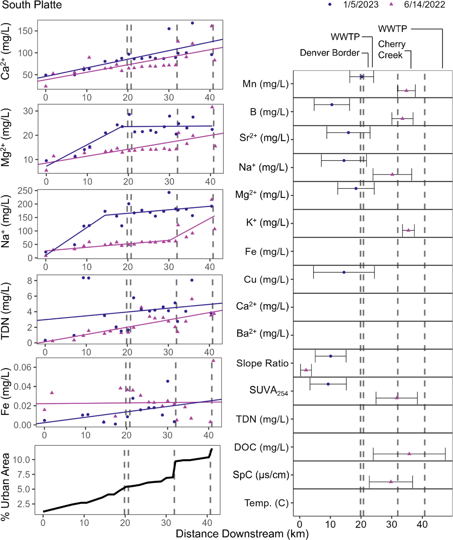
Na⁺, Ca²⁺, Mg²⁺, TDN, and Fe concentrations downstream for the South Platte. The locations and associated 95% confidence intervals of the breakpoints analyzed for every parameter. Circles represent the January 5, 2023 sampling date while triangles represent the June 14, 2022 sampling date. Note that y-axes are scaled relative to each concentration range. This is a two column figure. Figure was edited to fix font formatting issue.

In Bull Run, the salty chemical cocktails first followed an increasing typology and then are marked by two pulses potentially related to a quarry and wastewater effluent. B, Ca²⁺, Cu, Na⁺, Mg²⁺, K⁺, and Sr²⁺ all initially increased along the flowpath as Bull Run flowed through progressively more urban areas with rates ranging from 0.00017 to 2.4 mg L⁻¹ km⁻¹. Along Bull Run, there was a pulse then attenuation of Ca²⁺, Mg²⁺, Sr²⁺, and B 25–29 km downstream located near a quarry. TDN decreased along the flowpath until the wastewater treatment plant outfall, after which there was a pulse then attenuation in Na⁺, K⁺, and TDN. Ultimately, in both effluent influenced streams, there was a clear urbanization-related increase in salinity which is due to both effluent and other anthropogenic factors.

3.3.3. Increasing longitudinal trends and breakpoints in urbanizing streams influenced by geogenic salinity sources

Along the Licking River, the salty chemical cocktails followed a consistent increasing typology (Figure 5). The average breakpoint location for all ions roughly coincided with the region sampled for both dates, suggesting that variation between days drove differences in trends. Here, we report the trends downstream of the breakpoint as these reaches coincided more closely with the urbanization gradient. Ca²⁺, Mg²⁺, Na⁺, Sr²⁺, and K⁺ all increased along the flowpath at 0.00044 to 0.21 mg L⁻¹ km⁻¹. Na⁺ concentrations spiked and stabilized around the confluence of Banklick Creek, suggesting that this highly urban creek may contribute a localized pulse of Na⁺.

Figure 5.

Na⁺, Ca²⁺, Mg²⁺, TDN, and Fe concentrations downstream for the Licking River. The locations and associated 95% confidence intervals of the breakpoints analyzed for every parameter. Circles represent the January 30, 2023 sampling date while triangles represent the January 31, 2023 sampling date. Both dates were analyzed concurrently within the breakpoint analysis. Note that y-axes are scaled relative to each concentration range. This is a two column figure.

3.4. Parks and restoration are related to stable or decreasing trends in salty chemical cocktails

Although we generally observed increasing longitudinal trends in salty chemical cocktails with increasing urbanization, there were three streams with decreasing or stable trends as they flowed through parks and restoration areas (Scotts Level Branch, Northwest Anacostia, and Gwynns Falls). More specifically, the salty chemical cocktails in Scotts Level Branch decreased in concentration along the flowpath (Figure 6). Scotts Level Branch is a suburban stream that has several stream restoration projects along reaches, as well as a wider forested riparian zone. Na⁺, Cu, and K⁺ decreased consistently along the entire flowpath ranging from −1.9 to −0.00043 mg L⁻¹ km⁻¹ while Ca²⁺ was stable or slightly decreasing. Mg²⁺ and TDN decreased in the upstream reaches, where the stream restorations are located. Mg²⁺ had a breakpoint downstream of the second restoration at 4.0 ± 1.5 km downstream and TDN had a breakpoint after the first restoration at 0.89 ± 0.056 km downstream, then TDN and Mg²⁺ had stable or increasing trends in downstream, degraded reaches. Iron, a redox-sensitive element, followed an opposing trend, increasing throughout the restoration sites to 4.5 ± 1.4 km downstream, then decreasing for the rest of the degraded flowpath. These results suggested that, in the restored reaches, there was more floodplain connectivity where mobile, reduced iron was more prevalent, while in degraded reaches there was less floodplain connectivity (Kaushal et al., 2023a; Maas et al., 2023; Malin et al., 2024).

Figure 6.

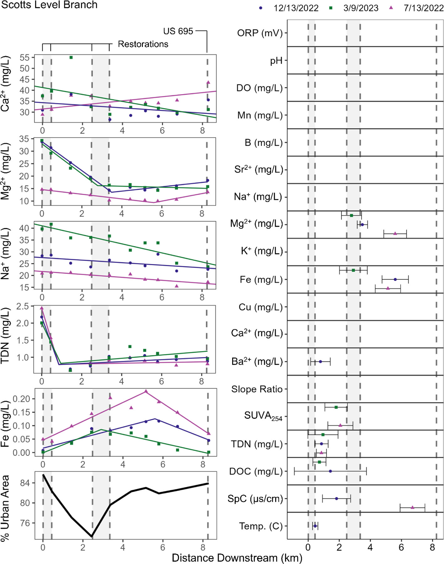
Na⁺, Ca²⁺, Mg²⁺, TDN, and Fe concentrations downstream for Scotts Level Branch. The locations and associated 95% confidence intervals of the breakpoints analyzed for every parameter. The shaded regions are the areas where Scotts Level Branch has been restored. Circles represent the December 12, 2023 sampling date, triangles represent the March 9, 2023 sampling date, and squares represent the July 13, 2022 sampling date. Note that y-axes are scaled relative to each concentration range. This is a two column figure.

The salty chemical cocktails in the Northwest Branch of the Anacostia River was decreasing or stable, demonstrating that parks and conservation areas may prevent urban impacts. The stream flows through the Rachel Carson Greenway and Burnt Mills Park, where, despite increasing urbanization in the watershed, the stream has a wide riparian buffer zone. Some elements were decreasing or stable along the entire flowpath, including Ca²⁺, Sr²⁺, and TDN. In July and December, Mg²⁺ had a breakpoint just after the start of the Rachel Carson Greenway at 15 ± 2.1 km downstream; after this point Mg²⁺ decreased (−0.28 to −0.12 mg L⁻¹ km⁻¹). Trends along the flowpath in Cu, Na⁺, and K⁺, including slopes, number of breakpoints, and breakpoint locations, were variable between seasons, but tended to be stable or increasing. Na⁺, Cu, K⁺, and Ca²⁺ all increased in concentration downstream of the confluence with Sligo Creek, suggesting that this tributary provided a localized pulse of ions.

Salty chemical cocktails generally increased longitudinally along the Gwynns Falls (Figure 7) but were attenuated when the stream flowed through a large forest conservation area at Leakin Park. Ca²⁺, Mg²⁺, and Na⁺ tended to increase along the flowpath, although there was some seasonal variability (see Supporting Info for the complete list of rates). Steeper linear increases in concentrations of weathering-related ions (Ca²⁺ and Mg²⁺) and less persistent increases in Na⁺ suggest that human-accelerated weathering is a main source of some anthropogenic ions in the Gwynns Falls watershed (Kaushal et al. 2017). The average breakpoint location across all parameters is 13.8 ± 4.3 km downstream, which coincided with Leakin Park, an extensive urban forest and conservation area. There were a variety of breakpoints and shifts in concentrations of Sr²⁺, TDN, K⁺, and Na⁺ in Leakin Park, indicating that this forested area likely influences water chemistry. During winter months, Na⁺ and Cu experienced a pulse at the last site, located under highways, indicating a potential road salt pulse. Given the conservation areas, presence of urban forests, and stream restoration involving stream-floodplain reconnection, the results from Scotts Level Branch, the Northwest Anacostia, and Gwynns Falls suggest that conservation and restoration features may have potential to attenuate elevated salt concentrations from urbanization (sensu Maas et al. 2023, Kaushal et al. 2023a).

Figure 7.

Na⁺, Ca²⁺, Mg²⁺, TDN, and Fe concentrations downstream for Gwynns Falls. The locations and associated 95% confidence intervals of the breakpoints analyzed for every parameter. The shaded area is the region where Gwynns Falls flows through Leakin Park. Circles represent the December 12, 2023 sampling date, triangles represent the March 9, 2023 sampling date, and squares represent the July 13, 2022 sampling date. Note that y-axes are scaled relative to each concentration range. This is a two column figure.

4. Discussion

Salinization represents a growing environmental concern across local, regional, and global scales (e.g., Cañedo-Argüelles et al., 2013; Dugan et al., 2017, Hintz et al., 2022, Kaushal et al. 2023a, 2021, 2005; Thorslund et al., 2021). In this study, we found that Ca²⁺, Mg²⁺, Na⁺, K⁺, Sr²⁺, TDN, and Cu were consistently related to one another, forming salty chemical cocktails across different streams and rivers draining five major U.S. metropolitan areas. Across metropolitan regions, there were consistently increasing longitudinal trends in salty chemical cocktails in streams and rivers along rural to urban flowpaths. These longitudinal trends showed distinct typologies of linear increases and plateaus (Kaushal et al., 2023a). Decreasing longitudinal trends as streams and rivers flowed through parks and restoration areas are similar to a growing body of work within the Chesapeake Bay region (Kaushal et al., 2023a; Maas et al., 2023; Malin et al., 2024). There were statistical breakpoints representing transitions in longitudinal trends influenced by urban boundaries, parks, and restoration and conservation zones. Our work illustrates the value of incorporating a watershed chemical cocktail approach of monitoring multiple elements simultaneously to characterize urban water quality signatures and track degradation and restoration of water quality. Below, we discuss the impacts of surrounding land use, underlying geology, and wastewater inputs on formation of chemical cocktails along stream flowpaths across different metropolitan regions. We also discuss how longitudinal trends and transitions in chemical cocktails can be attenuated on local scales by watershed management, riparian conservation, and stream-floodplain restoration.

4.1. Effects of urbanization on the formation of chemical cocktails

In our study, each longitudinal synoptic survey revealed a distinguishable chemical cocktail composed of salt ions and correlated elements. Na⁺, Ca²⁺, Mg²⁺, K⁺, Sr²⁺, and Cu were all frequently positively correlated with one another, and in many streams, TDN was also correlated. Our results suggest that there were distinct chemical cocktails formed along urban flowpaths, which can result from distinctly urban sources and processes. Principal component analysis revealed that these elements were related to one another across sites, forming salty chemical cocktails, and drove about half of the variability within the dataset. Overall, our results suggest that the transport and transformation of salts influences and/or co-mobilizes other elements creating close linkages among elements, which can be represented and visualized as chemical cocktail mixtures.

Our results are consistent with studies that describe how many salt ions follow similar patterns in sources and transport (Bhide et al., 2021; Haq et al., 2018; Kaushal et al., 2023c, 2020, 2017; Moore et al., 2017), but there can also be variations in the cycling of salts (Kaushal et al. 2023c). In natural environments, most major ions are controlled by similar weathering mechanisms (Gaillardet et al., 1999), while in urban environments, chemical cocktails form as multiple different chemical constituents (such as nutrients, salts, organic matter, and metals) can come from the same urban sources (E et al., 2023; Kaushal et al., 2023a, 2020, 2017; Maas et al., 2023). This watershed chemical cocktail approach allows us to understand which constituents are related biogeochemically to one another (Galella et al., 2021; Kaushal et al., 2020, 2019, 2018a; Morel et al., 2020) and reveals contaminant sources, sinks, and transformation processes relevant to water quality.

Many different urban sources and processes can contribute to chemical cocktails. For example, impervious surface cover increases runoff (Dunne and Leopold, 1978; Kaye et al., 2006), which flushes road salts, corroded metals, trash, nutrients, organic pollutants (such as polycyclic aromatic hydrocarbons), and pesticides into streams (Askarizadeh et al., 2015; Heaney and Sullivan, 1971; Kaushal et al., 2020; Masoner et al., 2019; McGrane, 2016; Paul and Meyer, 2001). Weathering, dissolution, and leaching of buildings, roads, and bridges releases base cations and carbonates that are transported to streams (Kaushal et al., 2020, 2017; Wright et al., 2011). In addition to increased runoff, changes in surface/subsurface hydrologic connectivity (e.g., water movement through storm drains bypassing riparian zones or leaky infrastructure interactions with groundwater) impact the formation of chemical cocktails (Kaushal and Belt, 2012; McGrane, 2016). These broader processes lead to the formation of salty chemical cocktails, although other processes more specifically describe how base cations, Sr²⁺, Cu, and TDN can be co-mobilized and transformed.

Geochemical and biogeochemical processes also enhance formation of chemical cocktails. Ion exchange leads to the mobilization of other cations and Cu when one cation is elevated (Galella et al., 2023a; Haq et al., 2018; Kaushal et al., 2017). Increases in salinity also increase ionic strength, which mobilizes hydrogen ions, thereby decreasing pH and influencing sediment dispersal (Haq et al., 2018; Kaushal et al., 2018b, 2017). Nitrogen can co-occur with these cations, as it can originate from the same urban sources such as effluent (Martí et al., 2010; 2004), be mobilized by ion exchange (Duan and Kaushal, 2015; Kaushal et al., 2017), and be partitioned between ammonium and nitrate differently due to salinization (Green et al., 2008). While this previous research describes how chemical cocktails can form in urban environments, this paper alongside other work contributes to the growing need to understand the role of salt ions as potential tracers of urbanization (Galella et al., 2021; Kaushal et al., 2020, 2019, 2018a; Morel et al., 2020).

4.2. Salty chemical cocktails can be a common signature of urbanization

We found consistent increasing trends in salty chemical cocktails (made up of Na⁺, Ca²⁺, Mg²⁺, K⁺, Sr²⁺, Cu, and sometimes TDN) across rural to urban gradients in seven streams flowing through five different metropolitan areas. The consistent formation of these salty chemical cocktails across cities and consistent increases in these salty chemical cocktails suggest that elevated salinity involving multiple different elements is a signature of urbanization. Other work has similarly shown that salinity tends to be elevated in urban areas, although most of the studies focus on specific conductance or one or two elements. Many urban streams have experienced chronic increases in salinity over time (Kaushal et al., 2018b), and increasing chloride concentrations have been observed across U.S. cities year-round related to urban development (Coles et al., 2012; Corsi et al., 2015; Kaushal et al., 2005; Moore et al., 2020; Stets et al., 2018). Increasing patterns in chloride with impervious surface cover are more pronounced in the northeastern U.S. compared to the southeastern U.S. due to higher usage rates of road salts (Moore et al., 2020). Road salts specifically have been linked to increasing specific conductance and Na⁺ and Cl⁻ concentrations throughout the U.S. (Coles et al., 2012; Cooper et al., 2014; Corsi et al., 2015, 2010; Kaushal et al., 2021, 2005; Moore et al., 2020). Other influences of urbanization such as wastewater inputs have been shown to increase salinity in regions that do not frequently use road salt (Rose, 2007). Spatially, specific conductance has also been shown to be elevated in urban areas when compared to rural areas (Brown et al., 2009). However, the impacts of urbanization depend on rural land use; urban signals tend to be stronger when compared to forested land use than when compared to agricultural land use (Brown et al., 2009; Reisinger et al., 2019). These urban increases in salinity across multiple ions in urban areas suggest that a chemical cocktail of salt is one signature of urbanization.

4.3. Increasing salty chemical cocktails were commonly found along rural to urban flowpaths

In this study, PCA results across nine streams and rivers suggested that there were different clusters of streams characterized by salty chemical cocktails representing influences from snowmelt, wastewater, geogenic salt sources, and weathering of impervious surfaces and road salt. Previous studies have established that climate, particularly aridity, can control solute concentrations (Li et al., 2022), however both our multiple linear regression and our longitudinal trends demonstrate that urbanization can also increase solutes across climate types. Our multiple linear regression revealed that across cities, salty chemical cocktails are influenced by urban land use and wastewater effluent in addition to climate and lithology. Our results show increased concentrations of many salt ions in urban areas in both the arid western and humid eastern U.S. Seven of nine studied urban streams had increasing longitudinal trends in salt ions, while the other two streams results were defined by parks and restoration areas. We found that there were increasing longitudinal trends of salty chemical cocktails along rural to urban gradients in streams and rivers, indicating that urbanization can drive increases in salinity.

We observed increasing longitudinal trends in salinization along streams and rivers as they flowed through progressively more urban areas. Previous longitudinal synoptic work has focused on smaller reach scales (Kaushal et al., 2023a; Maas et al., 2023), and our work expands this approach by focusing on urban stream flowpaths in larger watersheds and across metropolitan regions of the U.S. In seven of the nine streams studied, salt ions increased along stream flowpaths from rural to urban areas. There were increasing trends and plateaus in chemical cocktails of salt, TDN, Cu, and Sr²⁺. These trends were consistent across seasons, similar to other results suggesting spatial patterns are consistent over time (Wheeler and Ledford, 2023). There were also distinct transitions for multiple elements at sites coinciding with shifts in landscapes or management affecting multiple elements associated with salt. These results suggest that salty chemical cocktails can contribute to the overall geochemical signature of urbanization. The two streams that showed decreasing longitudinal trends and typologies have conservation and restoration features, which suggests that forest conservation areas, parks, and stream-floodplain restoration may disrupt the propagation of the salt signature further downstream through biogeochemical uptake, dilution, or hydrologic storage (see section 4.4.).

We observed increasing trends in salty chemical cocktails along the longitudinal flowpaths of Boulder Creek, Bull Run, Gwynns Falls, the Licking River, the South Platte River, Watts Branch, and the Willamette River. Increases in salinity from nonpoint sources in urban areas are often attributed to road salt application, weathering of impervious surfaces, and sewage leaks (Bain et al., 2012; Bhide et al., 2021; Brooks, 2014; Dailey et al., 2014; Hocking and Bailey, 2022; Kaushal et al., 2023a, 2022, 2017, 2011; Leslie and Lyons, 2018; Maas et al., 2023; Moore et al., 2017; Morel et al., 2020; Snodgrass et al., 2017). We observed these background increases in salinity across all seven sites with increasing typologies. Previous work has similarly shown that urbanization is related to elevated salinity either within or in the regions surrounding Boulder Creek (Barber et al., 2006; Nolan, 2020), Bull Run (Bhide et al., 2021; Maas et al., 2023), Gwynns Falls (Bain et al., 2012; Kaushal et al., 2023a, 2017, 2011; Kaushal and Belt, 2012; Moore et al., 2017; Snodgrass et al., 2017), the South Platte River (Hocking and Bailey, 2022; Litkey and Kimbrough, 1998), Watts Branch (Kaushal et al., 2023a, 2022; Maas et al., 2023; Morel et al., 2020), and the Willamette River (Waite et al., 2008). The one stream with additional non-urban drivers is the Licking River, where salt concentrations within the basin are largely attributed to the lithology, which is defined by shale, limestone, and salt licks (Carey, 2009; Fisher et al., 2007). However, urbanization has been shown to increase salinity in Kentucky and Ohio (Brooks, 2014; Dailey et al., 2014; Leslie and Lyons, 2018), and our observed pulse of Na⁺ likely originated from the urbanized Banklick Creek, suggesting that urbanization still plays a role in the Licking River salinity.

Point sources, specifically wastewater treatment plant effluent outfalls, also play a role in urban salt inputs. Consistent with other studies (Bhide et al., 2021; Maas et al., 2023), we observed how wastewater treatment plant effluent pulses elevate salinity in Bull Run. Effluent has also been shown to add salinity in the South Platte River (Dennehy et al., 1993; Haby and Loftis, 2012; Hocking and Bailey, 2022) and Boulder Creek (Barber et al., 2006; Murphy, 2006), and impact water quality in the Willamette River (Bloom, 2007). Wastewater treatment plant outfalls are located within our study area, thus this effluent likely contributes to increasing salinity observed across these sites. Across our study sites, nitrogen, phosphorus, pesticides, and organic contaminants have also been observed to increase in urban areas (Barber et al., 2006; Dennehy et al., 1998; Dougherty et al., 2006; Duan and Kaushal, 2013; Kaushal et al., 2011; Leland et al., 1997; Murphy, 2006; Waite et al., 2008). Elevated trace metals have been observed to be elevated in urban areas (Bain et al., 2012), and this pattern is present in our results as Cu is frequently included within the salty chemical cocktail. In Bull Run, the effluent pulse of Na⁺ coincides with elevated Cu, suggesting that some sources of salt are also sources of Cu. Additionally, ion exchange has been shown to mobilize Cu (Kaushal et al. 2019, Kaushal et al. 2022, Galella et al., 2023a,b). Across the seven sites with increasing longitudinal trends in salty chemical cocktails, this elevated salinity can generally be related to urbanization.

However, some of these streams have experienced localized increases in salinity relating to non-urban anthropogenic sources. In the South Platte, most previous work on salinity has focused downstream of Denver where increasing trends have been attributed to water reuse in agriculture. In this setting, evaporation, dissolution of soil minerals, and plant rejection of salts increase salinity (Dennehy et al., 1998; Haby and Loftis, 2012). In Bull Run, longitudinal pulses of Ca²⁺, Mg²⁺, and Sr²⁺ were likely influenced by the presence of a quarry, which has been shown to negatively impact the water quality in a nearby tributary Cub Run (Brent et al., 2022). Lastly, elevated groundwater salinities in the Licking River watershed have been attributed to brines from fossil fuel production (Carey, 2009; Fisher et al., 2007). Overall, anthropogenic activities elevate freshwater salinity in a wide variety of ways across cities, particularly in urban areas.

Spatial data, including longitudinal stream synoptics, provide understanding on how salts and other contaminants are loaded to streams (Byrne et al., 2017; Snodgrass et al., 2017). Within our work, the longitudinal stream synoptic data have provided insight on how water quality changes along rural to urban gradients, identified how abrupt changes in land use can influence water quality (such as the city border crossing in Boulder Creek), and located potential point sources (such as the wastewater treatment plant outfall and quarry in Bull Run). This type of data can reveal more information about the water quality impacts of channel morphology, the biogeochemical processing that occurs along flowpaths, how streams act as transporters and transformers of solutes, and how management approaches can attenuate contaminants along flowpaths (Mayer et al., 2022; Kaushal et al 2023a; Kaushal and Belt 2012). Longitudinal spatial data provides additional insights on what urban processes are occurring as spatial characteristics influence water quality. The way in which contaminant sources are located within and interact with the catchment influences how solutes are mobilized (Lintern et al., 2018). Land cover, land use, land management, atmospheric deposition, geology/soils, climate, topography, and hydrology influence the source, mobilization, and delivery of solutes (Lintern et al., 2018). House age, impervious surface extent, and stormwater connectivity have been shown to add variability in how urbanization impacts water quality (Carle et al., 2005). Urban infrastructure, such as storm drain pipe density, influences how urban-related increases in salinity change over time and at different flow conditions (Blaszczak et al., 2019). Ultimately, using longitudinal stream synoptic (LSS) monitoring data has allowed us to gain additional insight as to how urbanization impacts water chemistry, but more work is needed to fully understand how different spatial characteristics and biogeochemical processes mechanistically drive increases in salinity.

4.4. Parks and restoration can reduce urban water quality signatures and salinization

Urbanization-related increases in salinity pose larger water quality concerns, even though salt is a largely unregulated contaminant (Kaushal et al., 2021). Elevated salt concentrations can pose hazards to aquatic life (Hintz and Relyea, 2019), mobilize toxic metals such as copper and lead (Gallela et al., 2023a; Stets et al., 2018; Wilhelm et al., 2019), mobilize nitrogen and phosphorus (Green et al., 2008; Duan and Kaushal, 2015; Haq et al., 2018; Galella et al., 2023b), and pose direct threats to drinking water supplies, such as exceeding EPA recommended limits for sodium restricted diets (Kaushal et al., 2005; Grant et al., 2022). Thus there is a need to understand how elevated salinity can be managed within urban watersheds.

We observed decreasing or stable longitudinal trends in salty chemical cocktails at two sites with conservation and restoration features, suggesting that different watershed management strategies can play a role in attenuating urban salt pulses. Despite seasonal pulses of road salt and other increases of urbanization-related salinity in the Washington D.C. and Baltimore region (Kaushal et al., 2017; Moore et al., 2017), we found decreasing trends in salt ions along the flowpath of Scotts Level Branch consistent with other studies (Kaushal et al., 2023a; Maas et al., 2023; Malin et al., 2024). These decreases are related to stream restoration that promoted floodplain reconnection (Maas et al., 2023, Malin et al in review) and result in the attenuation of road salt pulses along the flowpath (Kaushal et al., 2023a; Maas et al., 2023). Load measurements suggest that these decreases in concentration are a result of attenuation, not only dilution (Malin et al., 2024). Retention and ion exchange can occur in sediments and floodplains at this site (Kaushal et al., 2023a, 2022), and increases in redox-sensitive elements alongside decreases in salt ion concentrations support retention within floodplains (Malin et al., 2024). Similarly, salt ions tended to decrease or have no trend along the flowpath of the Northwest Branch of the Anacostia River, despite increasing urban area along the flowpath, observed road salt pulses, and established urban sources of salinization in the Anacostia Watershed such as road salts and broken sewer lines (Galella et al., 2021; Haq et al., 2018; Miller et al., 2007). The Northwest Branch of the Anacostia River is surrounded by a large forested riparian buffer zone as it flows through the Rachel Carson Greenway and Burnt Mills Park. Forested portions of urban areas can increase infiltration and improve water quality (Berland et al., 2017); for the Northwest Branch of the Anacostia specifically, this conservation area likely limits urban road salt and infrastructure weathering sources of salts. Another mechanism for salt attenuation is the hydrologic retention of salts, where groundwater-surface water interactions have been shown to reduce salt pulses (Ledford and Lautz, 2014; Maas et al., 2021). The presence of parks and restoration areas in Scotts Level Branch and the Northwest Branch of the Anacostia River tempered the urban salty chemical cocktail.

The influence of parks and forest conservation areas on salt concentrations was also apparent in some of our sites with increasing typologies. In Gwynns Falls, many ions had breakpoints as the stream flowed through the Leakin Park. While this park was not large enough to disrupt overall increasing trends (Bain et al., 2012; Kaushal et al., 2023a, 2017; Kaushal and Belt, 2012), our more localized synoptic survey showed an influence on salt ions in the park. Leakin Park is an urban woodland that spans over 1,000 acres (City of Baltimore, 2015), where there is a lack of urban sources like road salt and weathering of the built environment (Kaushal et al., 2017). Similarly in Bull Run, concentrations of Na⁺, Ca²⁺, and Mg²⁺ decreased after their pulse-sources as the stream flowed through Bull Run Regional Park. While some of this could be due to dilution, downstream of the UOSA outflow Na⁺ is negatively related to Mg²⁺ and no longer positively related to Ca²⁺ (see Supporting Information), suggesting that ion exchange is attenuating Na⁺ along the flowpath. Additionally, the wide riparian buffer width within Bull Run Regional Park has been shown to drive the non-seasonal variance of salts (Maas et al., 2023). Overall, the presence of parks and restoration areas in the riparian zones of streams increases the potential for salty chemical cocktails to be attenuated along stream flowpaths.

4.5. Conclusions

In seven different streams across 5 different U.S. cities, we observed increasing salt concentrations along rural to urban flowpaths, suggesting that salinization can be a signature of urbanization. Our analysis of longitudinal stream synoptic monitoring data provided further insights regarding sources, sinks, transport, and transformation processes impacting pollutants in urban watersheds. In urban streams, we identified common chemical cocktails made up of Na⁺, Ca²⁺, Mg²⁺, K⁺, Cu, Sr²⁺, and TDN. Further, we found that salinity increased along flowpaths in seven of nine studied urban streams across the U.S. In the two streams with decreasing or stable longitudinal trends, parks and restoration areas were a noticeable component of land use. Identifying this salty, urbanization-related chemical cocktail, and utilizing a longitudinal stream synoptic approach is helpful in understanding the sources, transformation, and attenuation of stream contaminants. In the future, the chemical cocktail approach could potentially be utilized to understand urban contaminants as tracers of opportunity for tracking nonpoint and point source pollution. Thus, this approach and our results can be useful for water quality managers attempting to reduce urban stream contaminants, such as through implementation of best management practices or enforcement of total maximum daily loads (TMDLs). Although more work is needed, our results demonstrate that the chemical cocktail approach can be useful in identifying and tracking urbanization signatures, furthering our understanding of what urbanization processes and impacts are generalizable and what management strategies may be applicable across regions.

Highlights.

• Chemical mixtures of salt, nitrogen, and metals were tracked along streams

• Salty chemical cocktails formed along flowpaths

• Salty chemical cocktails typically increased along rural to urban flowpaths

• Salty chemical cocktails decreased through conservation and restoration areas

• Longitudinal patterns track sources, fate and transport of multiple pollutants

References

- Amrhein C, Strong JE, Mosher PA, 1992. Effect of Deicing Salts on Metal and Orgaic Matter Mobilization in Roadside Soils. Env. Sci Technol 26, 703–709. [Google Scholar]
- Anderson S, Jensen C, 2021. BCCZO -- Surface Water Chemistry -- (BC_SW_Array) -- Boulder Creek CZO -- (2008–2020) [WWW Document]. HydroShare URL https://www.hydroshare.org/resource/6938ed69fb704022b40b194426cc8302/ (accessed 9.12.23). [Google Scholar]
- Askarizadeh A, Rippy MA, Fletcher TD, Feldman DL, Peng J, Bowler P, Mehring AS, Winfrey BK, Vrugt JA, AghaKouchak A, Jiang SC, Sanders BF, Levin LA, Taylor S, Grant SB, 2015. From Rain Tanks to Catchments: Use of Low-Impact Development To Address Hydrologic Symptoms of the Urban Stream Syndrome. Environ. Sci. Technol 49, 11264–11280. 10.1021/acs.est.5b01635 [DOI] [PubMed] [Google Scholar]
- Bain DJ, Yesilonis ID, Pouyat RV, 2012. Metal concentrations in urban riparian sediments along an urbanization gradient. Biogeochemistry 107, 67–79. 10.1007/s10533-010-9532-4 [DOI] [Google Scholar]
- Balderas Guzman C, Wang R, Muellerklein O, Smith M, Eger CG, 2022. Comparing stormwater quality and watershed typologies across the United States: A machine learning approach. Water Research 216, 118283. 10.1016/j.watres.2022.118283 [DOI] [PubMed] [Google Scholar]
- Barber LB, Murphy SF, Verplanck PL, Sandstrom MW, Taylor HE, Furlong ET, 2006. Chemical Loading into Surface Water along a Hydrological, Biogeochemical, and Land Use Gradient: A Holistic Watershed Approach. Environ. Sci. Technol 40, 475–486. 10.1021/es051270q [DOI] [PubMed] [Google Scholar]
- Berland A, Shiflett SA, Shuster WD, Garmestani AS, Goddard HC, Herrmann DL, Hopton ME, 2017. The role of trees in urban stormwater management. Landscape and Urban Planning 162, 167–177. 10.1016/j.landurbplan.2017.02.017 [DOI] [PMC free article] [PubMed] [Google Scholar]
- Bhide SV, Grant SB, Parker EA, Rippy MA, Godrej AN, Kaushal S, Prelewicz G, Saji N, Curtis S, Vikesland P, Maile-Moskowitz A, Edwards M, Lopez KG, Birkland TA, Schenk T, 2021. Addressing the contribution of indirect potable reuse to inland freshwater salinization. Nat. Sustain 4, 699–707. 10.1038/s41893-021-00713-7 [DOI] [Google Scholar]
- Blaszczak JR, Delesantro JM, Zhong Y, Urban DL, Bernhardt ES, 2019. Watershed urban development controls on urban streamwater chemistry variability. Biogeochemistry 144, 61–84. 10.1007/s10533-019-00572-7 [DOI] [Google Scholar]
- Bloom JR, 2007. Willamette River Temperature Tmdl and River Model Presented at the TMDLS Conference 2007, Water Environment Federation, pp. 620–649. [Google Scholar]
- Bradley PM, Journey CA, Berninger JP, Button DT, Clark JM, Corsi SR, DeCicco LA, Hopkins KG, Huffman BJ, Nakagaki N, Norman JE, Nowell LH, Qi SL, VanMetre PC, Waite IR, 2019. Mixed-chemical exposure and predicted effects potential in wadeable southeastern USA streams. Sci. Total Environ 655, 70–83. 10.1016/j.scitotenv.2018.11.186 [DOI] [PubMed] [Google Scholar]
- Bradley PM, Journey CA, Romanok KM, Breitmeyer SE, Button DT, Carlisle DM, Huffman BJ, Mahler BJ, Nowell LH, Qi SL, Smalling KL, Waite IR, Van Metre PC, 2021. Multi-region assessment of chemical mixture exposures and predicted cumulative effects in USA wadeable urban/agriculture-gradient streams. Sci. Total Environ 773, 145062. 10.1016/j.scitotenv.2021.145062 [DOI] [PubMed] [Google Scholar]
- Brent RN, Kunkel J, Tomek Z, Buchardt D, DeLisle PF, Sivers S, 2022. A Novel Approach to Developing Thresholds for Total Dissolved Solids Using Standardized and Experimental Toxicity Test Methods. Environ. Toxicol. Chem 41, 2782–2796. 10.1002/etc.5466 [DOI] [PMC free article] [PubMed] [Google Scholar]
- Brooks JR, Wigington PJ Jr., Phillips DL, Comeleo R, Coulombe R, 2012. Willamette River Basin surface water isoscape (δ18O and δ2H): temporal changes of source water within the river. Ecosphere 3, art39. 10.1890/ES11-00338.1 [DOI] [Google Scholar]
- Brooks O, 2014. An analysis of the potential effects of urbanization on the water quality of the middle fork of Beargrass Creek, Louisville, Kentucky. University of Louisville. 10.18297/etd/158 [DOI] [Google Scholar]
- Brown LR, Cuffney TF, Coles JF, Fitzpatrick F, McMahon G, Steuer J, Bell AH, May JT, 2009. Urban streams across the USA: lessons learned from studies in 9 metropolitan areas. J. North Am. Benthol. Soc 28, 1051–1069. 10.1899/08-153.1 [DOI] [Google Scholar]
- Byrne P, Runkel RL, Walton-Day K, 2017. Synoptic sampling and principal components analysis to identify sources of water and metals to an acid mine drainage stream. Environmental Science and Pollution Research 24 (20), 17220–17240. 10.1007/s11356-017-9038-x [DOI] [PMC free article] [PubMed] [Google Scholar]
- Calcagno V 2020. glmulti: Model Selection and Multimodel Inference Made Easy [Google Scholar]
- Cañedo-Argüelles M, Kefford BJ, Piscart C, Prat N, Schäfer RB, Schulz C-J, 2013. Salinisation of rivers: An urgent ecological issue. Environ. Pollut 173, 157–167. 10.1016/j.envpol.2012.10.011 [DOI] [PubMed] [Google Scholar]
- Carey D, 2009. Licking River Basin. Ky. Geol. Surv. Map Chart 10.13023/kgs.mc191.12 [DOI] [Google Scholar]
- Carle MV, Halpin PN, Stow CA, 2005. Patterns of Watershed Urbanization and Impacts on Water Quality1. JAWRA J. Am. Water Resour. Assoc 41, 693–708. 10.1111/j.1752-1688.2005.tb03764.x [DOI] [Google Scholar]
- Chambers LG, Chin Y-P, Filippelli GM, Gardner CB, Herndon EM, Long DT, Lyons WB, Macpherson GL, McElmurry SP, McLean CE, Moore J, Moyer RP, Neumann K, Nezat CA, Soderberg K, Teutsch N, Widom E, 2016. Developing the scientific framework for urban geochemistry. Appl. Geochem 67, 1–20. 10.1016/j.apgeochem.2016.01.005 [DOI] [Google Scholar]
- Chang H, Pallathadka A, Sauer J, Grimm NB, Zimmerman R, Cheng C, Iwaniec DM, Kim Y, Lloyd R, McPhearson T, Rosenzweig B, Troxler T, Welty C, Brenner R, Herreros-Cantis P, 2021. Assessment of urban flood vulnerability using the social-ecological-technological systems framework in six US cities. Sustain. Cities Soc 68, 102786. 10.1016/j.scs.2021.102786 [DOI] [Google Scholar]
- City of Baltimore, 2015. Gwynns Falls/Leakin Park [WWW Document]. Dep. Recreat. Parks URL https://bcrp.baltimorecity.gov/parks/gwynns-falls (accessed 9.13.23). [Google Scholar]
- Coles JF, McMahon G, Bell AH, Brown LR, Fitzpatrick FA, Scudder Eikenberry BC, Woodside MD, Cuffney TF, Bryant WL, Cappiella K, Fraley-McNeal L, Stack WP, 2012. Effects of Urban Development on Stream Ecosystems in Nine Metropolitan Study Areas Across the United States: USGS Circular 1373 [Google Scholar]
- Cooper CA, Mayer PM, Faulkner BR, 2014. Effects of road salts on groundwater and surface water dynamics of sodium and chloride in an urban restored stream. Biogeochemistry 121, 149–166. 10.1007/s10533-014-9968-z [DOI] [Google Scholar]
- Cormier S, Wharton C, Olson J, 2021. U.S. EPA Freshwater Explorer. V: 0.1 United States Environmental Protection Agency. https://arcg.is/KHb9S [Google Scholar]
- Corsi SR, Graczyk DJ, Geis SW, Booth NL, Richards KD, 2010. A Fresh Look at Road Salt: Aquatic Toxicity and Water-Quality Impacts on Local, Regional, and National Scales. Environ. Sci. Technol 44, 7376–7382. 10.1021/es101333u [DOI] [PMC free article] [PubMed] [Google Scholar]
- Corsi SR, De Cicco LA, Lutz MA, Hirsch RM, 2015. River chloride trends in snow-affected urban watersheds: increasing concentrations outpace urban growth rate and are common among all seasons. Sci. Total Environ 508, 488–497. 10.1016/j.scitotenv.2014.12.012 [DOI] [PubMed] [Google Scholar]
- Crowley W, Reinhardt J, 1980. Geologic map of the Ellicot City quadrangle [Google Scholar]
- Dailey KR, Welch KA, Lyons WB, 2014. Evaluating the influence of road salt on water quality of Ohio rivers over time. Appl. Geochem 47, 25–35. 10.1016/j.apgeochem.2014.05.006 [DOI] [Google Scholar]
- Dennehy KF, Litke DW, Tate CM, Heiny JS, 1993. South Platte River Basin - Colorado, Nebraska, and Wyoming1. JAWRA J. Am. Water Resour. Assoc 29, 647–683. 10.1111/j.1752-1688.1993.tb03231.x [DOI] [Google Scholar]
- Dennehy KF, Litke DW, Tate CM, Qi SL, McMahon PB, Bruce BW, Kimbrough RA, Heiny JS, 1998. Water Quality in the South Platte River Basin, Colorado, Nebraska, and Wyoming, 1992–95: USGS Circular 1167, Circular [Google Scholar]
- Dodds WK, 2007. Trophic state, eutrophication and nutrient criteria in streams. Trends Ecol. Evol 22, 669–676. 10.1016/j.tree.2007.07.010 [DOI] [PubMed] [Google Scholar]
- Dougherty M, Dymond RL, Grizzard TJ, Godrej AN, Zipper CE, Randolph J, 2006. Quantifying Long-Term NPS Pollutant Flux in an Urbanizing Watershed. J. Environ. Eng 132, 547–554. 10.1061/(ASCE)0733-9372(2006)132:4(547) [DOI] [Google Scholar]
- Duan S, Kaushal SS, 2013. Warming increases carbon and nutrient fluxes from sediments in streams across land use. Biogeosciences 10, 1193–1207. 10.5194/bg-10-1193-2013 [DOI] [Google Scholar]
- Duan S, Kaushal SS, 2015. Salinization alters fluxes of bioreactive elements from stream ecosystems across land use. Biogeosciences 12, 7331–7347. 10.5194/bg-12-7331-2015 [DOI] [Google Scholar]
- Dugan HA, Bartlett SL, Burke SM, Doubek JP, Krivak-Tetley FE, Skaff NK, Summers JC, Farrell KJ, McCollough IM, Morales-Williams AM, Roberts DC, Ouyang Z, Scordo F, Hanson PC, Weahers KC, 2017. Salting our freshwater lakes. PNAS 114 (17), 4453–4458. 10.1073/pnas.1620211114 [DOI] [PMC free article] [PubMed] [Google Scholar]
- Dunne T, Leopold LB, 1978. Water in Environmental Planning Macmillan. [Google Scholar]
- E, B., Zhang S, Driscoll CT, Wen T, 2023. Human and natural impacts on the U.S. freshwater salinization and alkalinization: A machine learning approach. Sci. Total Environ 889, 164138. 10.1016/j.scitotenv.2023.164138 [DOI] [PubMed] [Google Scholar]
- Ehalt Macedo H, Lehner B, Nicell J, Grill G, Li J, Limtong A, Shakya R 2022. Distribution and characteristics of wastewater treatment plants within the global river network. Earth System Science Data, 14(2): 559–577. 10.5194/essd-14-559-2022 [DOI] [Google Scholar]
- Evans-White MA, Haggard BE, Scott JT, 2013. A review of stream nutrient criteria development in the United States. J. Environ. Qual 42, 1002–1014. 10.2134/jeq2012.0491 [DOI] [PubMed] [Google Scholar]
- Farid S, Baloch MK, Ahmad SA, 2012. Water pollution: Major issue in urban areas. Int. J. Water Resour. Environ. Eng 4, 55–65. 10.5897/IJWREE11.086 [DOI] [Google Scholar]
- Field A, Miles J, Field Z, 2012. Discovering statistics using R, Repr. ed Sage, Los Angeles, CA, USA. [Google Scholar]
- Fisher R, Davidson B, Goodmann P, 2007. Groundwater Quality in Watersheds of the Kentucky River, Salt River, Licking River, Big Sandy River, Little Sandy River, and Tygarts Creek (Kentucky Basin Management Units 1, 2, and 5). Ky. Geol. Surv. Rep. Investig 10.13023/kgs.ri16.12 [DOI] [Google Scholar]
- Fox J, Weisberg S, Price B, Adler D, Bates D, Baud-Bovy G, Bolker B, Ellison S, Firth D, Friendly M, Gorjanc G, Graves S, Heiberger R, Krivitsky P, Laboissiere R, Maechler M, Monette G, Murdoch D, Nilsson H, Ogle D, Ripley B, Short T, Venables W, Walker S, Winsemius D, Zeileis A, R-Core, 2023. car: Companion to Applied Regression [Google Scholar]
- Gabor RS, Hall SJ, Eiriksson DP, Jameel Y, Millington M, Stout T, Barnes ML, Gelderloos A, Tennant H, Bowen GJ, Neilson BT, Brooks PD, 2017. Persistent Urban Influence on Surface Water Quality via Impacted Groundwater. Environ. Sci. Technol 51, 9477–9487. 10.1021/acs.est.7b00271 [DOI] [PubMed] [Google Scholar]
- Gaillardet J, Dupré B, Louvat P, Allègre CJ, 1999. Global silicate weathering and CO2 consumption rates deduced from the chemistry of large rivers. Chem. Geol 159, 3–30. 10.1016/S0009-2541(99)00031-5 [DOI] [Google Scholar]
- Galella JG, Kaushal SS, Wood KL, Reimer JE, Mayer PM, 2021. Sensors track mobilization of ‘chemical cocktails’ in streams impacted by road salts in the Chesapeake Bay watershed. Environ. Res. Lett 16, 035017. 10.1088/1748-9326/abe48f [DOI] [PMC free article] [PubMed] [Google Scholar]
- Galella JG, Kaushal SS, Mayer PM, Maas CM, Shatkay RR, Stutzke RA, 2023a. Stormwater best management practices: Experimental evaluation of chemical cocktails mobilized by freshwater salinization syndrome. Front. Environ. Sci 11. 10.3389/fenvs.2023.1020914 [DOI] [PMC free article] [PubMed] [Google Scholar]
- Galella JG, Kaushal SS, Mayer PM, Maas CM, Shatkay RR, Inamdar S, Belt KT, 2023b. Freshwater Salinization Syndrome Alters Nitrogen Transport in Urban Watersheds. Water 15(22), 3956. 10.3390/w15223956 [DOI] [PMC free article] [PubMed] [Google Scholar]
- Grant SB, Rippy MA, Birkland TA, Schenk T, Rowles K, Misra S, Aminpour P, Kaushal S, Vikesland P, Berglund E, Gomez-Velez JD, Hotchkiss ER, Perez G, Zhang HX, Armstrong K, Bhide SV, Krauss L, Maas C, Mendoza K, Shipman C, Zhang Y, Zhong Y, 2022. Can Common Pool Resource Theory Catalyze Stakeholder-Driven Solutions to the Freshwater Salinization Syndrome? Environ. Sci. Technol 56, 13517–13527. 10.1021/acs.est.2c01555 [DOI] [PMC free article] [PubMed] [Google Scholar]
- Green SM, Machin R, Cresser MS, 2008. Effect of long-term changes in soil chemistry induced by road salt applications on N-transformations in roadside soils. Environ. Pollut 152, 20–31. 10.1016/j.envpol.2007.06.005 [DOI] [PubMed] [Google Scholar]
- Grimm NB, Faeth SH, Golubiewski NE, Redman CL, Wu J, Bai X, Briggs JM, 2008. Global Change and the Ecology of Cities. Science 319, 756–760. 10.1126/science.1150195 [DOI] [PubMed] [Google Scholar]
- Groemping U, Lehrkamp M 2023. Relaimpo: Relative Importance of Regressors in Linear Models [Google Scholar]
- Groffman PM, Rosi E, Martel LD, 2020. Baltimore Ecosystem Study: Stream chemistry for core sites in Gwynns Falls 10.6073/PASTA/45129DA171F2A8AB5A96E9743D0D644B [DOI] [Google Scholar]
- Haby PA, Loftis JC, 2012. Salinity Characterization and Source Assessment in the South Platte River Basin, Northeastern Colorado 1–7. 10.1061/40499(2000)132 [DOI] [Google Scholar]
- Haq S, Kaushal SS, Duan S, 2018. Episodic salinization and freshwater salinization syndrome mobilize base cations, carbon, and nutrients to streams across urban regions. Biogeochemistry 141, 463–486. 10.1007/s10533-018-0514-2 [DOI] [Google Scholar]
- Harrell FE Jr, Dupont C, 2023. Hmisc: Harrell Miscellaneous [Google Scholar]
- Heaney JP, Sullivan RH, 1971. Source Control of Urban Water Pollution. J. Water Pollut. Control Fed 43, 571–579. [PubMed] [Google Scholar]
- Helms JR, Stubbins A, Ritchie JD, Minor EC, Kieber DJ, Mopper K, 2008. Absorption spectral slopes and slope ratios as indicators of molecular weight, source, and photobleaching of chromophoric dissolved organic matter. Limnol. Oceanogr 53, 955–969. 10.4319/lo.2008.53.3.0955 [DOI] [Google Scholar]
- Hill Ryan A., Weber Marc H., Leibowitz Scott G., Olsen Anthony R., and Thornbrugh Darren J., 2016. The Stream-Catchment (StreamCat) Dataset: A Database of Watershed Metrics for the Conterminous United States. Journal of the American Water Resources Association (JAWRA) 52:120–128. 10.1111/1752-1688.12372. [DOI] [Google Scholar]
- Hintz WD, Relyea RA, 2019. A review of the species, community, and ecosystem impacts of road salt salinisation in fresh waters. Freshwater Biology 64 (6), 1081–1097. 10.1111/fwb.13286 [DOI] [Google Scholar]
- Hintz WD, Arnott SE, Symons CC, Greco DA, McClymont A, Brentrup JA, Cañedo-Argüelles M, Derry AM, Downing AL, Gray DK, Melles SJ, Relyea RA, Rusak JA, Searle CL, Astorg L, Baker HK, Beisner BE, Cottingham KL, Ersoy Z, Espinosa C, Franceschini J, Giorgio AT, Göbeler N, Hassal E, Hébert M-P, Huynh M, Hylander S, Jonasen KL, Kirkwood AE, Langenheder S, Langvall O, Laudon H, Lind L, Lundgren M, Proia L, Schuler MS, Shurin JB, Steiner CF, Striebel M, Thibodeau S, Urrutia-Cordero P, Vendrell-Puigmitja L, Weyhenmeyer GA, 2022. Current water quality guidelines across North America and Europe do not protect lakes from salinization. Proceedings of the National Academy of Sciences 119, e2115033119. 10.1073/pnas.2115033119 [DOI] [PMC free article] [PubMed] [Google Scholar]
- Hocking C, Bailey RT, 2022. Salt transport in a large agro-urban river basin: Modeling, controlling factors, and management strategies. Front. Water 4. 10.3389/frwa.2022.945682 [DOI] [Google Scholar]
- Hopkins KG, Morse NB, Bain DJ, Bettez ND, Grimm NB, Morse JL, Palta MM, 2015a. Type and timing of stream flow changes in urbanizing watersheds in the Eastern U.S. Elem. Sci. Anthr 3, 000056. 10.12952/journal.elementa.000056 [DOI] [Google Scholar]
- Hopkins KG, Morse NB, Bain DJ, Bettez ND, Grimm NB, Morse JL, Palta MM, Shuster WD, Bratt AR, Suchy AK, 2015b. Assessment of Regional Variation in Streamflow Responses to Urbanization and the Persistence of Physiography. Environ. Sci. Technol 49, 2724–2732. 10.1021/es505389y [DOI] [PubMed] [Google Scholar]
- Hu C, Muller-Karger FE, Zepp RG, 2002. Absorbance, absorption coefficient, and apparent quantum yield: A comment on common ambiguity in the use of these optical concepts. Limnol. Oceanogr 47, 1261–1267. 10.4319/lo.2002.47.4.1261 [DOI] [Google Scholar]
- Husson F, Josse J, Le S, Mazet J, 2023. FactoMineR: Multivariate Exploratory Data Analysis and Data Mining [Google Scholar]
- Kassambara A, Mundt F, 2020. factoextra: Extract and Visualize the Results of Multivariate Data Analyses [Google Scholar]
- Kaushal SS, Groffman PM, Likens GE, Belt KT, Stack WP, Kelly VR, Band LE, Fisher GT, 2005. Increased salinization of fresh water in the northeastern United States. Proc. Natl. Acad. Sci 102, 13517–13520. 10.1073/pnas.0506414102 [DOI] [PMC free article] [PubMed] [Google Scholar]
- Kaushal SS, Groffman PM, Band LE, Elliott EM, Shields CA, Kendall C, 2011. Tracking Nonpoint Source Nitrogen Pollution in Human-Impacted Watersheds. Environ. Sci. Technol 45, 8225–8232. 10.1021/es200779e [DOI] [PubMed] [Google Scholar]
- Kaushal SS, Belt KT, 2012. The urban watershed continuum: evolving spatial and temporal dimensions. Urban Ecosyst 15, 409–435. 10.1007/s11252-012-0226-7 [DOI] [Google Scholar]
- Kaushal SS, McDowell WH, Wollheim WM, 2014a. Tracking evolution of urban biogeochemical cycles: past, present, and future. Biogeochemistry 121, 1–21. 10.1007/s10533-014-0014-y [DOI] [Google Scholar]
- Kaushal SS, Delaney-Newcomb K, Findlay SEG, Newcomer TA, Duan S, Pennino MJ, Sivirichi GM, Sides-Raley AM, Walbridge MR, Belt KT, 2014b. Longitudinal patterns in carbon and nitrogen fluxes and stream metabolism along an urban watershed continuum. Biogeochemistry 121, 23–44. 10.1007/s10533-014-9979-9 [DOI] [Google Scholar]
- Kaushal SS, Duan S, Doody TR, Haq S, Smith RM, Newcomer Johnson TA, Newcomb KD, Gorman J, Bowman N, Mayer PM, Wood KL, Belt KT, Stack WP, 2017. Human-accelerated weathering increases salinization, major ions, and alkalinization in fresh water across land use. Appl. Geochem., Urban Geochemistry 83, 121–135. 10.1016/j.apgeochem.2017.02.006 [DOI] [PMC free article] [PubMed] [Google Scholar]
- Kaushal SS, Gold AJ, Bernal S, Johnson TAN, Addy K, Burgin A, Burns DA, Coble AA, Hood E, Lu Y, Mayer P, Minor EC, Schroth AW, Vidon P, Wilson H, Xenopoulos MA, Doody T, Galella JG, Goodling P, Haviland K, Haq S, Wessel B, Wood KL, Jaworski N, Belt KT, 2018a. Watershed ‘chemical cocktails’: forming novel elemental combinations in Anthropocene fresh waters. Biogeochemistry 141, 281–305. 10.1007/s10533-018-0502-6 [DOI] [PMC free article] [PubMed] [Google Scholar]
- Kaushal SS, Likens GE, Pace ML, Utz RM, Haq S, Gorman J, Grese M, 2018b. Freshwater salinization syndrome on a continental scale. Proc. Natl. Acad. Sci 115, E574–E583. 10.1073/pnas.1711234115 [DOI] [PMC free article] [PubMed] [Google Scholar]
- Kaushal SS, Likens GE, Pace ML, Haq S, Wood KL, Galella JG, Morel C, Doody TR, Wessel B, Kortelainen P, Räike A, Skinner V, Utz R, Jaworski N, 2019. Novel ‘chemical cocktails’ in inland waters are a consequence of the freshwater salinization syndrome. Philos. Trans. R. Soc. B Biol. Sci 374, 20180017. 10.1098/rstb.2018.0017 [DOI] [PMC free article] [PubMed] [Google Scholar]
- Kaushal SS, Wood KL, Galella JG, Gion AM, Haq S, Goodling PJ, Haviland KA, Reimer JE, Morel CJ, Wessel B, Nguyen W, Hollingsworth JW, Mei K, Leal J, Widmer J, Sharif R, Mayer PM, Newcomer Johnson TA, Newcomb KD, Smith E, Belt KT, 2020. Making ‘chemical cocktails’ – Evolution of urban geochemical processes across the periodic table of elements. Appl. Geochem 119, 104632. 10.1016/j.apgeochem.2020.104632 [DOI] [PMC free article] [PubMed] [Google Scholar]
- Kaushal SS, Likens GE, Pace ML, Reimer JE, Maas CM, Galella JG, Utz RM, Duan S, Kryger JR, Yaculak AM, Boger WL, Bailey NW, Haq S, Wood KL, Wessel BM, Park CE, Collison DC, Aisin B.Y. ‘aaqob I., Gedeon TM, Chaudhary SK, Widmer J, Blackwood CR, Bolster CM, Devilbiss ML, Garrison DL, Halevi S, Kese GQ, Quach EK, Rogelio CMP, Tan ML, Wald HJS, Woglo SA, 2021. Freshwater salinization syndrome: from emerging global problem to managing risks. Biogeochemistry 154, 255–292. 10.1007/s10533-021-00784-w [DOI] [Google Scholar]
- Kaushal SS, Reimer JE, Mayer PM, Shatkay RR, Maas CM, Nguyen WD, Boger WL, Yaculak AM, Doody TR, Pennino MJ, Bailey NW, Galella JG, Weingrad A, Collison DC, Wood KL, Haq S, Newcomer-Johnson TA, Duan S, Belt KT, 2022. Freshwater salinization syndrome alters retention and release of chemical cocktails along flowpaths: From stormwater management to urban streams. Freshw. Sci 41, 420–441. 10.1086/721469 [DOI] [PMC free article] [PubMed] [Google Scholar]
- Kaushal SS, Maas CM, Mayer PM, Newcomer-Johnson TA, Grant SB, Rippy MA, Shatkay RR, Leathers J, Gold AJ, Smith C, McMullen EC, Haq S, Smith R, Duan S, Malin J, Yaculak A, Reimer JE, Delaney Newcomb K, Sides Raley A, Collison DC, Galella JG, Grese M, Sivirichi G, Doody TR, Vikesland P, Bhide SV, Krauss L, Daugherty M, Stavrou C, Etheredge M, Ziegler J, Kirschnick A, England W, Belt KT, 2023a. Longitudinal stream synoptic monitoring tracks chemicals along watershed continuums: a typology of trends. Front. Environ. Sci 11. 10.3389/fenvs.2023.1122485 [DOI] [PMC free article] [PubMed] [Google Scholar]
- Kaushal SS, Mayer PM, Likens GE, Reimer JE, Maas CM, Rippy MA, Grant SB, Hart I, Utz RM, Shatkay RR and Wessel BM, 2023b. Five state factors control progressive stages of freshwater salinization syndrome. Limnology and Oceanography Letters, 8(1), pp.190–211. [DOI] [PMC free article] [PubMed] [Google Scholar]
- Kaushal SS, Likens GE, Mayer PM, Shatkay RR, Shelton SA, Grant SB, Utz RM, Yaculak AM, Maas CM, Reimer JE, Bhide SV, Malin JT, Rippy MA, 2023c. The anthropogenic salt cycle. Nat. Rev. Earth Environ 1–15. 10.1038/s43017-023-00485-y [DOI] [PMC free article] [PubMed] [Google Scholar]
- Kaushal SS, Fork ML, Hawley RJ, Hopkins KG, Ríos-Touma B, Roy AH, 2023d. Stream restoration milestones: monitoring scales determine successes and failures. Urban Ecosyst 26, 1131–1142. 10.1007/s11252-023-01370-8 [DOI] [Google Scholar]
- Kaye JP, Groffman PM, Grimm NB, Baker LA, Pouyat RV, 2006. A distinct urban biogeochemistry? Trends Ecol. Evol 21, 192–199. 10.1016/j.tree.2005.12.006 [DOI] [PubMed] [Google Scholar]
- Kolpin DW, Furlong ET, Meyer MT, Thurman EM, Zaugg SD, Barber LB, Buxton HT, 2002. Pharmaceuticals, Hormones, and Other Organic Wastewater Contaminants in U.S. Streams, 1999−2000: A National Reconnaissance. Environ. Sci. Technol 36, 1202–1211. 10.1021/es011055j [DOI] [PubMed] [Google Scholar]
- Ledford SH, Lautz LK, 2015. Floodplain connection buffers seasonal changes in urban stream water quality. Hydrological Processes 29 (6), 1002–1016. 10.1002/hyp.10210 [DOI] [Google Scholar]
- Leland D, Anderson S, Sterling DJ Jr., 1997. The Willamette—a river in peril. J. AWWA 89, 73–83. 10.1002/j.1551-8833.1997.tb08323.x [DOI] [Google Scholar]
- Leslie DL, Lyons WB, 2018. Variations in Dissolved Nitrate, Chloride, and Sulfate in Precipitation, Reservoir, and Tap Waters, Columbus, Ohio. Int. J. Environ. Res. Public. Health 15, 1752. 10.3390/ijerph15081752 [DOI] [PMC free article] [PubMed] [Google Scholar]
- Li L, Stewart B, Zhi W, Sadayappan K, Ramesh S, Kerins D, Sterle G, Harpold A, Perdrial J, 2022. Climate Controls on River Chemistry. Earths Future 10, e2021EF002603. 10.1029/2021EF002603 [DOI] [Google Scholar]
- Lindsey DA, Langer WH, Knepper DH, 2005. Stratigraphy, lithology, and sedimentary features of Quaternary alluvial deposits of the South Platte River and some of its tributaries east of the Front Range, Colorado: U.S. Geological Survey Professional Paper 1705 (Professional Paper), Professional Paper [Google Scholar]
- Lintern A, Webb J. a., Ryu D, Liu S, Bende-Michl U, Waters D, Leahy P, Wilson P, Western AW, 2018. Key factors influencing differences in stream water quality across space. WIREs Water 5, e1260. 10.1002/wat2.1260 [DOI] [Google Scholar]
- Litkey DW, Kimbrough RA, 1998. Water-quality assessment of the South Platte River Basin, Colorado, Nebraska, and Wyoming: Environmental setting and water quality of fixed sites, 1993–95. 10.3133/wri974220 [DOI] [Google Scholar]
- Löfgren S, 2001. The Chemical Effects of Deicing Salt on Soil and Stream Water of Five Catchments in Southeast Sweden. Water. Air. Soil Pollut 130, 863–868. 10.1023/A:1013895215558 [DOI] [Google Scholar]
- Maas CM, Anderson WP, Cockerill K, 2021. Managing Stormwater by Accident: A Conceptual Study. Water 13(11), 1492. 10.3390/w13111492 [DOI] [Google Scholar]
- Maas CM, Kaushal SS, Rippy MA, Mayer PM, Grant SB, Shatkay RR, Malin JT, Bhide SV, Vikesland P, Krauss L, Reimer JE, Yaculak AM, 2023. Freshwater salinization syndrome limits management efforts to improve water quality. Front. Environ. Sci 11. 10.3389/fenvs.2023.1106581 [DOI] [PMC free article] [PubMed] [Google Scholar]
- Malin JT, Kaushal SS, Mayer PM, Maas CM, Hohman S, Rippy M, 2024. Longitudinal Stream Synoptic (LSS) Monitoring to Evaluate Water Quality in Restored Streams. Environ. Monit. Assess 196:437. 10.1007/s10661-024-12570-w [DOI] [PMC free article] [PubMed] [Google Scholar]
- Martí E, Aumatell J, Godé L, Poch M, Sabater F, 2004. Nutrient Retention Efficiency in Streams Receiving Inputs from Wastewater Treatment Plants. Journal of Environmental Quality 33(1), 285–293. 10.2134/jeq2004.2850 [DOI] [PubMed] [Google Scholar]
- Martí E, Riera JL, Sabater F, Sabater S, Barceló D, 2010. Effects of Wastewater Treatment Plants on Stream Nutrient Dynamics Under Water Scarcity Conditions. The Handbook of Environmental Chemistry, 173–195. 10.1007/698_2009_33 [DOI] [Google Scholar]
- Masoner JR, Kolpin DW, Cozzarelli IM, Barber LB, Burden DS, Foreman WT, Forshay KJ, Furlong ET, Groves JF, Hladik ML, Hopton ME, Jaeschke JB, Keefe SH, Krabbenhoft DP, Lowrance R, Romanok KM, Rus DL, Selbig WR, Williams BH, Bradley PM, 2019. Urban Stormwater: An Overlooked Pathway of Extensive Mixed Contaminants to Surface and Groundwaters in the United States. Environ. Sci. Technol 53, 10070–10081. 10.1021/acs.est.9b02867 [DOI] [PMC free article] [PubMed] [Google Scholar]
- Mayer PM, Pennino MJ, Newcomer-Johnson TA, Kaushal SS, 2022. Long-term assessment of floodplain reconnection as a stream restoration approach for managing nitrogen in ground and surface waters. Urban Ecosystems 25 (3), 879–907. 10.1007/s11252-021-01199-z [DOI] [PMC free article] [PubMed] [Google Scholar]
- Mazerolle MJ, 2023. AICcmodavg: Model Selection and Multimodel Inference Based on (Q)AIC(c) [Google Scholar]
- McGrane SJ, 2016. Impacts of urbanisation on hydrological and water quality dynamics, and urban water management: a review. Hydrol. Sci. J 61, 2295–2311. 10.1080/02626667.2015.1128084 [DOI] [Google Scholar]
- McPhearson T, Pickett STA, Grimm NB, Niemelä J, Alberti M, Elmqvist T, Weber C, Haase D, Breuste J, Qureshi S, 2016. Advancing Urban Ecology toward a Science of Cities. BioScience 66, 198–212. 10.1093/biosci/biw002 [DOI] [Google Scholar]
- Miller CV, Gutierrez-Magness AL, Feit Majedi BL, Foster GD, 2007. Water Quality in the Upper Anacostia River, Maryland: Continuous and Discrete Monitoring with Simulations to Estimate Concentrations and Yields, 2003–05: U.S. Geological Survey Scientific Investigations Report 2007–5142. [Google Scholar]
- Moore J, Bird DL, Dobbis SK, Woodward G, 2017. Nonpoint Source Contributions Drive Elevated Major Ion and Dissolved Inorganic Carbon Concentrations in Urban Watersheds. Environ. Sci. Technol. Lett 4, 198–204. 10.1021/acs.estlett.7b00096 [DOI] [Google Scholar]
- Moore J, Fanelli RM, Sekellick AJ, 2020. High-Frequency Data Reveal Deicing Salts Drive Elevated Specific Conductance and Chloride along with Pervasive and Frequent Exceedances of the U.S. Environmental Protection Agency Aquatic Life Criteria for Chloride in Urban Streams. Environ. Sci. Technol 54, 778–789. 10.1021/acs.est.9b04316 [DOI] [PubMed] [Google Scholar]
- Morel CJ, Kaushal SS, Tan ML, Belt KT, 2020. Developing Sensor Proxies for “Chemical Cocktails” of Trace Metals in Urban Streams. Water 12, 2864. 10.3390/w12102864 [DOI] [Google Scholar]
- Muggeo VMR, 2023. segmented: Regression Models with Break-Points / Change-Points (with Possibly Random Effects) Estimation [Google Scholar]
- Murphy S, 2006. State of the watershed: water quality of Boulder Creek, Colorado: USGS Circular 1284 (Circular), Circular https://pubs.usgs.gov/circ/circ1284/ [Google Scholar]
- Newcomer Johnson TA, Kaushal SS, Mayer PM, Grese MM, 2014. Effects of stormwater management and stream restoration on watershed nitrogen retention. Biogeochemistry 121, 81–106. 10.1007/s10533-014-9999-5 [DOI] [Google Scholar]
- Nolan A, 2020. Temporal and Spatial Analysis of Anthropogenic Impact to Boulder Creek Water Quality (M.S. Thesis) University of Colorado Boulder. [Google Scholar]
- O’Connor JE, Mangano JF, Anderson SW, Wallick JR, Jones KL, Keith MK, 2014. Geologic and physiographic controls on bed-material yield, transport, and channel morphology for alluvial and bedrock rivers, western Oregon. GSA Bull 126, 377–397. 10.1130/B30831.1 [DOI] [Google Scholar]
- Parr TB, Cronan CS, Danielson TJ, Tsomides L, Simon KS, 2016. Aligning indicators of community composition and biogeochemical function in stream monitoring and ecological assessments. Ecol. Indic 60, 970–979. 10.1016/j.ecolind.2015.08.049 [DOI] [Google Scholar]
- Paul MJ, Meyer JL, 2001. Streams in the Urban Landscape. Annu. Rev. Ecol. Syst 32, 333–365. 10.1146/annurev.ecolsys.32.081501.114040 [DOI] [Google Scholar]
- Peña-Guzmán C, Ulloa-Sánchez S, Mora K, Helena-Bustos R, Lopez-Barrera E, Alvarez J, Rodriguez-Pinzón M, 2019. Emerging pollutants in the urban water cycle in Latin America: A review of the current literature. J. Environ. Manage 237, 408–423. 10.1016/j.jenvman.2019.02.100 [DOI] [PubMed] [Google Scholar]
- Pennino MJ, Kaushal SS, Mayer PM, Utz RM, Cooper CA, 2016a. Stream restoration and sewers impact sources and fluxes of water, carbon, and nutrients in urban watersheds. Hydrol. Earth Syst. Sci 20, 3419–3439. 10.5194/hess-20-3419-2016 [DOI] [Google Scholar]
- Pennino MJ, Kaushal SS, Murthy SN, Blomquist JD, Cornwell JC, Harris LA, 2016b. Sources and transformations of anthropogenic nitrogen along an urban river–estuarine continuum. Biogeosciences 13, 6211–6228. 10.5194/bg-13-6211-2016 [DOI] [Google Scholar]
- Reisinger AJ, Woytowitz E, Majcher E, Rosi EJ, Belt KT, Duncan JM, Kaushal SS, Groffman PM, 2019. Changes in long-term water quality of Baltimore streams are associated with both gray and green infrastructure. Limnology and Oceanography 64 (S1), S60–S76. 10.1002/lno.10947 [DOI] [Google Scholar]
- Ripley B, Venables B, Bates DM, Hornik K, Gebhardt A, Firth D 2024. MASS: Support Functions and Datasets for Venables and Ripley’s MASS [Google Scholar]
- Rose S, 2007. The effects of urbanization on the hydrochemistry of base flow within the Chattahoochee River Basin (Georgia, USA). J. Hydrol 341, 42–54. 10.1016/j.jhydrol.2007.04.019 [DOI] [Google Scholar]
- Shelton S, Neale P, Pinsonneault A, Tzortziou M, 2022. Biodegradation and Photodegradation of Vegetation-Derived Dissolved Organic Matter in Tidal Marsh Ecosystems. Estuaries Coasts 45, 1324–1342. 10.1007/s12237-021-00982-7 [DOI] [Google Scholar]
- Sivirichi GM, Kaushal SS, Mayer PM, Welty C, Belt KT, Newcomer T, Newcomb KD, Grese MM, 2011. Longitudinal variability in streamwater chemistry and carbon and nitrogen fluxes in restored and degraded urban stream networks. J. Environ. Monit 13, 288–303. 10.1039/C0EM00055H [DOI] [PubMed] [Google Scholar]
- Snodgrass JW, Moore J, Lev SM, Casey RE, Ownby DR, Flora RF, Izzo G, 2017. Influence of Modern Stormwater Management Practices on Transport of Road Salt to Surface Waters. Environ. Sci. Technol 51, 4165–4172. 10.1021/acs.est.6b03107 [DOI] [PubMed] [Google Scholar]
- Southworth S, Denenny D, 2006. Geologic map of the National Parks in the National Capital Region, Washington, D.C., Virginia, Maryland, and West Virginia: U.S. Geological Survey Open-File Report 2005–1331 (Open-File Report), Open-File Report [Google Scholar]
- Stets EG, Lee CJ, Lytle DA, Schock MR, 2018. Increasing chloride in rivers of the conterminous U.S. and linkages to potential corrosivity and lead action level exceedances in drinking water. Sci. Total Environ 613–614, 1498–1509. 10.1016/j.scitotenv.2017.07.119 [DOI] [PMC free article] [PubMed] [Google Scholar]
- Thorslund J, Bierkens MFP, Oude Essink GHP, Sutanudjaja EH, van Vliet MTH, 2021. Common irrigation drivers of freshwater salinisation in river basins worldwide. Nature Communications 12(1), 4232. 10.1038/s41467-021-24281-8 [DOI] [PMC free article] [PubMed] [Google Scholar]
- Tong STY, Chen W, 2002. Modeling the relationship between land use and surface water quality. J. Environ. Manage 66, 377–393. 10.1006/jema.2002.0593 [DOI] [PubMed] [Google Scholar]
- Tyler RH, Boyer TP, Minami T, Zweng MM, Reagan JR, 2017. Electrical conductivity of the global ocean. Earth Planets Space 69, 156. 10.1186/s40623-017-0739-7 [DOI] [PMC free article] [PubMed] [Google Scholar]
- U.S. Geological Survey, 2016. National Water Information System data available on the World Wide Web (USGS Water Data for the Nation) [WWW Document] URL https://waterdata.usgs.gov/nwis (accessed 11.3.23).
- U.S. Geological Survey, 2019a. The StreamStats program [WWW Document] URL https://streamstats.usgs.gov/ss/ (accessed 11.3.23).
- U.S. Geological Survey, 2019b. National Hydrography Dataset, TNM Download (v2.0) [WWW Document] URL https://apps.nationalmap.gov/downloader/#/ (accessed 11.3.23).
- Waite IR, Sobieszczyk S, Carpenter KD, Arnsberg AJ, Johnson HM, Hughes CA, Sarantou MJ, Rinella FA, 2008. Effects of Urbanization on Stream Ecosystems in the Willamette River Basin and Surrounding Area, Oregon and Washington: U.S. Geological Survey Scientific Investigations Report 2006-5101-D [Google Scholar]
- Walsh CJ, Roy AH, Feminella JW, Cottingham PD, Groffman PM, Morgan RP, 2005. The urban stream syndrome: current knowledge and the search for a cure. J. North Am. Benthol. Soc 24, 706–723. 10.1899/04-028.1 [DOI] [Google Scholar]
- Wei T, Simko V, Levy M, Xie Y, Jin Y, Zemla J, Freidank M, Cai J, Protivinsky T, 2021. corrplot: Visualization of a Correlation Matrix [Google Scholar]
- Weishaar JL, Aiken GR, Bergamaschi BA, Fram MS, Fujii R, Mopper K, 2003. Evaluation of Specific Ultraviolet Absorbance as an Indicator of the Chemical Composition and Reactivity of Dissolved Organic Carbon. Environ. Sci. Technol 37, 4702–4708. 10.1021/es030360x [DOI] [PubMed] [Google Scholar]
- Wheeler CT, Ledford SH, 2023. Stability in headwater chemical signatures across a dynamic flow regime in a highly urbanized Piedmont catchment. Hydrological Processes 37 (2), e14825. 10.1002/hyp.14825 [DOI] [Google Scholar]
- Wilhelm JF, Bain DJ, Green MB, Bush KF, McDowell WH, 2019, Trace metals in Northern New England streams: Evaluating the role of road salt across broad spatial scales with synoptic snapshots. PLOS ONE 14 (2), e0212011. 10.1371/journal.pone.0212011 [DOI] [PMC free article] [PubMed] [Google Scholar]
- Wright IA, Davies PJ, Findlay SJ, Jonasson OJ, Wright IA, Davies PJ, Findlay SJ, Jonasson OJ, 2011. A new type of water pollution: concrete drainage infrastructure and geochemical contamination of urban waters. Mar. Freshw. Res 62, 1355–1361. 10.1071/MF10296 [DOI] [Google Scholar]
Associated Data
This section collects any data citations, data availability statements, or supplementary materials included in this article.