Establishment of quadratic exponential quality gain-loss function model and design of process mean

Abstract

Taking into account the fluctuation of the growth rate on the left and right sides of the classic QGLF, a quadratic exponential quality gain-loss function (QGLF) is created based on the asymmetric QGLF. The two scenarios of non-normal distribution (triangular distribution) and truncated normal distribution of quality characteristic values are optimized using the quadratic exponential quality gain-loss process mean. Through the case study approaches, the empirical validity and applicability of the quadratic exponential QGLF model are thoroughly assessed, confirming its effectiveness in improving quality management practices.

1. Introduction

After decades of research, the loss function—which was widely used for quality loss prediction—has shown promising outcomes in decision-making, quality engineering, tolerance design, and other domains. The most well-known of these is the quadratic quality loss function, which was put forth by Japanese quality management scientist Dr. Genichi Taguchi. According to Taguchi, the loss a product causes society after it is listed and it will always experience loss if it deviates from the target value [1]. Spring et al. designed an inverse normal quality loss function to address the unbounded nature of the Taguchi loss function. This new function removes the restriction on specification limits, making it more applicable in practical scenarios [2]. Xue Li delved into enhancing quality control through the integration of the quality loss function with the economic design of ARMA and VSI EWMA control charts [3,4]. Meanwhile, Li Yaping et al. aimed to refine quality loss prediction by refining the quality loss function to make it dimensionless. Leveraging orthogonal tests, they devised a stochastic grey-target model for multi-quality characteristic parameter design in products, tackling the challenge of selecting parameters for products with multiple quality characteristics [5]. To arrive at a more robust optimal solution, Zhang Liuyang et al. employed the mass loss function for multi-response robust parameter design and optimization [6]. Feng Zebiao and colleagues tackle the challenge of document parameter design to mitigate model prediction bias and fluctuation. They devise a multi-response optimization model by integrating the mass loss function within the framework of multivariate Gaussian process modeling [7]. Zhai Cuihong and colleagues employ a novel approach, leveraging the Prize Fast non-separable Gaussian process in conjunction with a multivariate mass-loss function. This methodology is applied to devise a two-stage parameter optimization scheme, utilizing nonlinear optimization algorithms to identify the optimal joint parameter design values for space and time factors [8]. Khawarita Siregar et al. used Taguchi's quality loss function for quality assessment to calculate the loss due to product dimensional variations, determining the long-dimensional process capability index required for a company to meet the desired specifications [9]. Mao et al. conducted research on the reliability issues of components. They improved the Taguchi function to address the problem of growth rates on both sides of the target value. Building on this, they proposed a reliability prediction model for implicit quality costs and studied the impact of different parameters on product reliability [10]. Li Shuangshuang and colleagues extended the Taylor expansion to the third order to develop a cubic quality loss function. They also examined the quality loss coefficient and suggested using the cubic loss function to calculate hidden quality costs [11]. Zheng Yuqiao and colleagues concentrated on the quality control issues of wind turbine hub assembly. They took into account both the production costs and the relative quality losses, established loss standards for quality characteristics, and improved the loss function. Building on this, they conducted the identification of key processes [12]. Numerous production procedures demonstrate that, in addition to quality loss, there are occasionally quality gain effects brought about by quality compensation during the manufacturing process [[13], [14], [15]]. With the intention of examining the impact of quality compensation in real-world manufacturing, Wang Bo et al. introduced the idea of QGLF and used it to define the constant term in the Taylor expansion as the meaning of compensation. The function model of the big and small loss of the first term under the constant compensation amount is proposed when the quality compensation amount is constant and aims at the loss of the QGLF first term. The QGLF is applied to test the quality properties of construction of dam concrete, and its compensation form is studied. To enhance the conventional techniques of controlling the quality of dam concrete, the target planning model is built and the tolerance design of concrete construction is improved taking the influence of compensation amount into account. Since data sources are widely used in quality control procedures, data accuracy is frequently not guaranteed. The inverse normal grey QGLF model, which analyzed the two existence cases of compensation amount and constructed the grey QGLF model with the properties close to target, maximum, and minimum values, is proposed. Typically, the target value is determined by past experience or hypothesis. The current process capability indexes are compared and examined, the disposal table and classification standard are created, and the process capacities are represented by six times the typical standard deviation. The grey QGLF is utilized to determine the optimal engineering specifications for both loss and compensation conditions separately [[16], [17], [18], [19]]. Nie Xiangtian et al. created a fuzzy QGLF model by analyzing fuzziness in the quality control process practically and by using related fuzzy mathematics concepts. They then created the optimal method average of the binary asymmetric QGLF using a triangular distribution probability density function [20]. In order to deal with the defects in traditional quality gain-loss functions, which typically overlook primary and tertiary term losses, Wangbo has developed an advanced tertiary quality gain-loss function model. This innovative model not only provides a tertiary asymmetric quality gain-loss function but also integrates a sophisticated gain-loss cost model based on both constant and hyperbolic tangent compensation strategies [21].

Many domestic scholars have conducted extensive research in the field of process quality control, proposing numerous effective improvements and achieving notable results in studying process capability and control charts. For example, Jin Qiu posits that asymmetric quality loss can be mitigated through optimization. By examining four scenarios of triangular distribution, she revised the process mean optimization model and explored the optimal process mean in asymmetric contexts [22]. Zhao et al. developed a new tolerance design method that incorporates factors such as the operating environment by using the quality loss function and applied tolerance design theory to the service stage [23]. Khawarita Siregar et al. applied Taguchi's quality loss function to quality assessment, calculating the loss incurred by the company due to product dimensional variations necessary to meet the desired specifications [24].

The uneven rates of quality gain and loss around a goal value are usually not taken into consideration by existing Quality Gain-Loss Function (QGLF) models. It's possible that this mistake misrepresents the complex dynamics in some engineering situations. This research suggests that the pace of quality change on both sides of a target value can be asymmetric under certain conditions. For example, an intriguing pattern appears in the temperature control systems used in the laying of concrete during dam construction: when the concrete's outlet temperature falls below the target, the rate at which quality diminishes increases; conversely, if the outlet temperature exceeds the target, this rate of quality degradation slows and eventually plateaus. Beyond a certain upper limit, the material is deemed unsuitable and subject to rework or rejection.

The rate of quality degradation in concrete increases as the concrete's outlet temperature drops below the objective; on the other hand, if the concrete's outlet temperature rises above the target, the rate of quality degradation slows and eventually plateaus. The content is considered inappropriate and may be rejected or changed if it goes beyond a certain point.

In order to reconcile this disparity, we present a new quadratic exponential QGLF model that takes into account this asymmetry, paying special attention to situations in which the quality change acts differently across the goal value threshold. In order to determine the ideal process mean design, we investigate the consequences of this model using truncated normal and triangular distributions as a lens. This method provides a strong framework for improving quality control in engineering projects with comparable features and provides a more nuanced knowledge of quality-loss dynamics under both normal and non-normal distributions.

2. Quadratic exponential quality gain-loss function

2.1. Quality gain-loss function

The quality gain-loss function is developed based on Taguchi's quality loss function. This concept, proposed by Genichi Taguchi, a renowned quality expert from Japan, posits that a product incurs “no loss” only when its characteristics match the target precisely. Even a slight deviation from the target results in a quality loss, and this loss escalates with increasing deviation from the target. Essentially, the quality loss is minimized and considered zero when the quality characteristic meets the target value. However, any deviation from the target value will generate a quality loss, as expressed in Equation (1).

$$L\left(y\right)=k{\left(y-m\right)}^2$$ (1)

As the Taguchi quality loss function has seen increasingly widespread application, its limitations have become apparent. In response, numerous scholars have conducted extensive research to address the drawbacks of the Taguchi quality loss function, such as its unboundedness, asymmetry, and multivariable issues.

Wang Bo argues that extensive production practices have demonstrated that processes are mutually compensating and adaptive coupling processes. Given the premise of quality loss, there is also a quality gain effect due to quality compensation between processes. Wang Bo introduced the quality gain-loss function (QGLF) by incorporating the constant term from the Taylor series expansion as a quality compensation term and omitting higher-order terms beyond the second order. The QGLF is derived as follows:

$$G\left(y\right)=G\left(m\right)+k_2{\left(y-m\right)}^2$$ (2)

$$k_2=\left[A_0-G\left(m\right)\right]/{{\Delta }_0}^2=\left[A-G\left(m\right)\right]/{\xi }^2$$ (3)

In the formula, $G\left(y\right)$ represents the corresponding quality gain-loss value when the product quality characteristic value is y; $k_2=G^{″}\left(m\right)/2！$ is a constant; $G\left(m\right)$ is real number R. Since the loss function has a minimum quality loss of 0 when y = m, so $G\left(m\right)$ can be expressed as the maximum quality profit, which is called quality compensation. The image of the QGLF is shown in Fig. 1:

Fig. 1.

Image of QGLF

2.2. Piecewise quality gain-loss function

Wang Bo et al. applied the piecewise function theory to establish the piecewise function QGLF model in view of the asymmetry of quality gain-loss in actual production [16]:

$$G_f\left(y\right)=\{\begin{array}{l}{g}_f\left(y\right)+k_{f1}{\left(y-m\right)}^2，y\le m\\ g_f\left(y\right)+k_{f2}{\left(y-m\right)}^2，y>m\end{array}$$ (4)

In the formula: k_f1、k_f2 are the quality loss coefficients.

If $g_f\left(y\right)=a_f\left(\text{constant}\right)$, the piecewise QGLF curve is shown in Fig. 2.

Fig. 2.

Piecewise QGLF curve.

2.3. Quadratic exponential quality gain-loss function

The rate of change of mass loss on the left and right sides of the goal value is not taken into account by the traditional asymmetric QGLF. On the other hand, there are several scenarios for the rate of change of quality loss on both sides of the QGLF's objective value in response to various production techniques; that is, the QGLF's growth rate increases when y < m and drops when y > m.

This study builds the following QGLF by taking into account the growth rates on both sides of the goal value:

$$L\left(x\right)=\{\begin{array}{l}g\left(y\right)+A_1,y<T_l\\ g\left(y\right)+k_1{\left(y-m\right)}^2,T_l<y<m\\ g\left(y\right)+k_2\left(1-e^{-y+m}\right)，m<y<T_u\\ g\left(y\right)+A_2,y>T_u\end{array}$$ (5)

Where: $g\left(y\right)$ represents the quality compensation amount, m is the target characteristic value, $T_l$ and $T_u$ are the lower and upper functional limits of the product, respectively. $A_1$ indicates the quality gain-loss value below the lower limit, $A_2$ indicates the quality gain-loss value above the upper limit. The quality gain–loss coefficients k₁ and k₂ are obtained as follows:

$$\begin{array}{l}{k}_1=\frac{A_1}{{\left(T_l-m\right)}^2}\\ k_2=\frac{A_2}{\left(1-e^{-y+m}\right)}\end{array}$$ (6)

The diagram of the quadratic exponential QGLF is shown in Fig. 3.

Fig. 3.

Image of quadratic exponential QGLF.

3. Optimal process mean design in triangular distribution

Triangular distributions have a wide range of applications, especially in risk analysis, project management, resource allocation, and quality control. By modeling uncertainty as a triangular distribution, potential risks and variability can be better understood, leading to more accurate and reliable decisions.

Chen et al. put forward that if Y₁ and Y₂ are random variables that are mutually independent and uniformly distributed, then the probability density function of Y=Y1+Y2 under the triangular distribution is as follows:

$$F\left(y\right)=\{\begin{array}{r}\frac{2\left(y-a-x\right)}{\left(b-a\right)\left(c-a\right)}a+x\le y<b+x\\ \frac{2\left(c+x-y\right)}{\left(c-b\right)\left(c-a\right)}b+x\le y<c+x\\ 0y<a+xory>c+x\end{array}$$ (7)

Where: T is the tolerance value, a is the minimum value of random variable Y, a = m-T; b is the intermediate value of random variable Y, b = m; c means the maximum value of random variable Y, c = m + T; x represents the distance between the process mean and the target value.

The probability density function of the triangular distribution is shown as follows:

$$F\left(y\right)=\{\begin{array}{r}\frac{y-m+T-x}{T^2}a+x\le y<b+x\\ \frac{m+T+x-y}{T^2}b+x\le y<c+x\\ 0y<a+xory>c+x\end{array}$$ (8)

The quality gain-loss value of batch products is expressed by expectation as follows:

$$E\left(\mathrm{L}\right)={\int }_{Tl}^{m}F\left(y\right)\left[w+k_1{\left(y-m\right)}^2\right]dy+{\int }_m^{Tu}F\left(y\right)\left[w+k_2\left(1-e^{-y+m}\right)\right]dy$$ (9)

3.1. Triangular distribution case 1 (see Fig. 4)

Fig. 4.

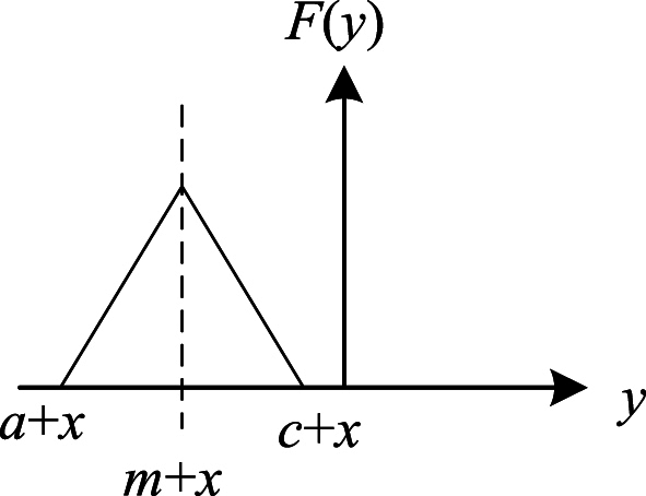
Schematic diagram of triangular distribution case 1.

In case 1, $c+x\le m$, i.e. $x\le -T$, the expected gain-loss obtained from equation (8) (9) is as follows:

$$E=\frac{1}{T^2}\{{\int }_{a+x}^{m+x}\left(y-m+T-x\right)\left[w+k_1{\left(y-m\right)}^2\right]dy+{\int }_{m+x}^{c+x}\left(m+T+x-y\right)\left[w+k_1{\left(y-m\right)}^2\right]\}=w+k_1{x}^2+\frac{k_1{T}^2}{6}$$ (10)

The minimum point of equation (11) is x matching the criteria of k1>k2, as the precondition states that when k1>k2, the second derivative is greater than 0, i.e. $E^{\prime }=2K_{1}x=0$, indicating that the first derivative is a convex function about x. Currently, the ideal process mean is x + m. Where: m represents the target characteristic value; T is the tolerance value, a is the minimum value of random variable Y; c is the maximum value of random variable Y; x is the distance between the process mean and the target value, k₁ is the quality gain–loss coefficient.

3.2. Triangular distribution case 2 (see Fig. 5)

Fig. 5.

Schematic diagram of triangular distribution case 2.

In case 2, $m+x\le m<c+x$, i.e. $-T<x<0$, the expected gain-loss obtained from equation (8) (9) is as follows:

$$E=\frac{1}{T^2}\{{\int }_{a+x}^{m+x}\left(y-m+T-x\right)\left[w+k_1{\left(y-m\right)}^2\right]dy+{\int }_{m+x}^m\left(m+T+x-y\right)\left[w+k_1{\left(y-m\right)}^2\right]dy+{\int }_m^{c+x}\left(m+T+x-y\right)\left[w+k_2\left(1-e^{-y+m}\right)\right]dy\}=\frac{k_1}{T^2}\left[-\frac{x^4}{6}+\frac{{\left(x-T\right)}^4}{12}\right]+\frac{k_2}{T^2}\left[\frac{{\left(T+x\right)}^2}{2}-\frac{e^T}{e^x}-T-x+1\right]+w$$ (11)

Find the first derivative of equation (10) with respect to x and make it 0 to get the following equation:

$$\frac{dE}{dx}=\frac{k_1}{T^2}\left\{-\frac{2}{3}{x}^3+\frac{{\left(x-T\right)}^3}{3}\right\}+\frac{k_2}{T^2}\left\{\left(T+x\right)+e^T\frac{1}{e^x}-1\right\}=0$$ (12)

Find the second derivative of equation (11) with respect to x to obtain the following equation:

$$\frac{d^{2}E}{d{x}^2}=\frac{k_1}{T^2}\left[-2x^2+{\left(x-T\right)}^2\right]+\frac{k_2}{T^2}\left[1-\frac{e^T}{e^x}\right]$$ (13)

According to the precondition $-T<x<0$, when k₁>k₂, the second derivative is greater than 0, so the first derivative is a convex function about x, so x meeting the conditions of k₁>k₂ and equation (12) is the minimum point of equation (11). At present, x + m is the optimal process mean.

Where: m represents the target characteristic value; T is the tolerance value, a is the minimum value of random variable Y; c is the maximum value of random variable Y; x is the distance between the process mean and the target value, k₁ is the quality gain–loss coefficient (left side), k₂ is the quality gain–loss coefficient (right side).

3.3. Triangular distribution case 3 (see Fig. 6)

Fig. 6.

Schematic diagram of triangular distribution case 3.

In case 3, $a+x\le m<m+x$, i.e. $0<x<T$ , the expected gain-loss can be obtained from Equations (8), (9) as follows:

$$E=\frac{1}{T^2}\{{\int }_{a+x}^m\left(y-m+T-x\right)\left[w+k_1{\left(y-m\right)}^2\right]dy\}+\frac{1}{T^2}\{{\int }_m^{m+x}\left(m+T+x-y\right)\left[w+\left(1-e^{-y+m}\right)\right]dy+{\int }_{m+x}^{c+x}\left(m+T+x-y\right)\left[w+k_2\left(1-e^{-y+m}\right)\right]dy\}=\frac{k_1}{T^2}\frac{{\left(x-T\right)}^4}{12}+\frac{k_2}{T^2}\left[\frac{2}{e^x}-1+T+x+\frac{T^2}{2}+Tx-\frac{x^2}{2}-\frac{1}{e^{T+x}}\right]+w$$ (14)

Find the first derivative of equation (14) with respect to x and make it 0 to get the following equation:

$$\frac{dE}{dx}=\frac{k_1}{T^2}\frac{{\left(x-T\right)}^3}{3}+\frac{k_2}{T^2}\left[-\frac{2}{e^x}+1+T-x+\frac{1}{e^{T+x}}\right]$$ (15)

Find the second derivative of equation (14) with respect to x to obtain the following equation:

$$\frac{d^{2}E}{d{x}^2}=\frac{k_1}{T^2}{\left(x-T\right)}^2+\frac{k_2}{T^2}\left[\frac{2}{e^x}-1-\frac{1}{e^{T+x}}\right]$$ (16)

According to the precondition $0<x<T$, when k₁>k₂, the second derivative is greater than 0 and the first derivative is a convex function about x, so x meets the conditions of k₁>k₂ and equation (15) is the minimum point of equation (14). At present, x + m is the optimal process mean.

Where: m represents the target characteristic value; T is the tolerance value, a is the minimum value of random variable Y; c is the maximum value of random variable Y; x is the distance between the process mean and the target value, k₁ is the quality gain–loss coefficient (left side), k₂ is the quality gain–loss coefficient (right side).

3.4. Triangular distribution case 4 (see Fig. 7)

Fig. 7.

Schematic diagram of triangular distribution case 4.

In case 4, $a+x\ge m$, i.e. x ≥ T, the expected gain-loss can be obtained from Equations (8), (9) as follows:

$$E=\frac{1}{T^2}\{{\int }_{a+x}^{m+x}\left(y-m+T-x\right)\left[w+k_2\left(1-e^{-y+m}\right)\right]dy+{\int }_{m+x}^{c+x}\left(m+T+x-y\right)\left[w+k_2\left(1-e^{-y+m}\right)\right]\}=w+\frac{k_2}{T^2}\left(-\frac{2}{e^x}-\frac{e^T}{e^x}+T^2-\frac{1}{e^T}\frac{1}{e^x}\right)$$ (17)

Find the first derivative of equation (17) with respect to x and make it 0 to get the following equation:

$$\frac{dE}{dx}=\frac{k_2}{T^2}\left(-\frac{2}{e^x}+\frac{e^T}{e^x}+\frac{1}{e^T}\frac{1}{e^x}\right)=0$$ (18)

When T = x = 0, equation (18) holds, but x = 0 is not in the definition domain, so this point is not the optimal process mean point.

Where: m represents the target characteristic value; T is the tolerance value, a is the minimum value of random variable Y; c is the maximum value of random variable Y; x is the distance between the process mean and the target value, k₁ is the quality gain–loss coefficient (left side), k₂ is the quality gain–loss coefficient (right side).

4. Optimal process mean design under normal distribution

This research uses truncated normal distribution for process mean design since there will be particular intervals for the selection of quality characteristic values in real-world engineering applications. Under the truncated normal distribution, three process mean design models are created based on the various ranges of characteristic value intervals.

4.1. Truncated normal distribution

Given a quality characteristic value of y and a value range of $\left({\zeta }_1，{\zeta }_2\right)$, the probability density function g(y) and distribution function G(y) of y are represented by equation (19):

$$\begin{array}{c}G\left(y\right)=P\left(Y\le y|{\zeta }_1\le y\le {\zeta }_2\right)=\frac{F\left(y\right)-F\left({\zeta }_1\right)}{F\left({\zeta }_2\right)-F\left({\zeta }_1\right)}\\ g\left(y\right)=\frac{f\left(y\right)}{F\left({\zeta }_2\right)-F\left({\zeta }_1\right)}\end{array}$$ (19)

Where, f(y)is the probability density function of normal distribution.

4.2. Optimal process mean design model under truncated normal distribution

When the product quality characteristics are within the upper and lower functional limits, the expected gain-loss is:

$$E_1={\int }_{T_l}^m\left[k_1{\left(y-m\right)}^2+w\right]g\left(y\right)dy+{\int }_m^{T_u}\left[k_2\left(1-\exp \left(-y+m\right)\right)+w\right]g\left(y\right)dy$$ (20)

When the product quality characteristics are below the lower functional limit or above the upper functional limit, the expected gain-loss is:

$$E_2={\int }_{{\zeta }_1}^{T_l}\left(A_1+w\right)g\left(y\right)dy+{\int }_{T_u}^{{\zeta }_2}\left(A_2+w\right)g\left(y\right)dy$$ (21)

Therefore, the total expected gain-loss is:

$$E=E_1+E_2=\frac{1}{F\left({\zeta }_2\right)-F\left({\zeta }_1\right)}[A_1{\int }_{{\zeta }_1}^{T_l}f\left(y\right)dy+k_1{m}^2{\int }_{T_l}^{m}f\left(y\right)dy+k_2{\int }_m^{T_u}f\left(y\right)dy+A_2{\int }_{T_u}^{{\zeta }_2}f\left(y\right)dy+k_1{\int }_{T_l}^m{y}^{2}f\left(y\right)dy-2m{k}_1{\int }_{T_l}^{m}yf\left(y\right)dy-k_2{\int }_m^{T_u}\exp \left(-y+m\right)f\left(y\right)dy]+w_0$$ (22)

When ${\zeta }_2\to +\infty$, the probability density function of quality characteristic y is:

$$g\left(y\right)=\frac{f\left(y\right)}{1-F\left({\zeta }_1\right)}$$ (23)

In this case, the expected gain-loss is:

$$E=E_1+E_2=\frac{1}{1-F\left({\zeta }_1\right)}[A_1{\int }_{{\zeta }_1}^{T_l}f\left(y\right)dy+k_1{m}^2{\int }_{T_l}^{m}f\left(y\right)dy+k_2{\int }_m^{T_u}f\left(y\right)dy+A_2{\int }_{T_u}^{+\infty }f\left(y\right)dy+k_1{\int }_{T_l}^m{y}^{2}f\left(y\right)dy-2m{k}_1{\int }_{T_l}^{m}yf\left(y\right)dy-k_2{\int }_m^{T_u}\exp \left(-y+m\right)f\left(y\right)dy]+w_1$$ (24)

When ${\zeta }_1\to -\infty$, i.e. the value range of y has no lower limit, the expected quality gain-loss in this case is:

$$E=E_1+E_2=\frac{1}{F\left({\zeta }_2\right)}[A_1{\int }_{-\infty }^{T_l}f\left(y\right)dy+k_1{m}^2{\int }_{T_l}^{m}f\left(y\right)dy+k_2{\int }_m^{T_u}f\left(y\right)dy+A_2{\int }_{T_u}^{{\zeta }_2}f\left(y\right)dy+k_1{\int }_{T_l}^m{y}^{2}f\left(y\right)dy-2m{k}_1{\int }_{T_l}^{m}yf\left(y\right)dy-k_2{\int }_m^{T_u}\exp \left(-y+m\right)f\left(y\right)dy]+w_2$$ (25)

When ${\zeta }_1\to -\infty 、{\zeta }_2\to +\infty$, i.e. the value range of y has no upper or lower limit, then y is a complete normal distribution. In this case, the expected gain-loss is:

$$E=E_1+E_2=[A_1{\int }_{-\infty }^{T_l}f\left(y\right)dy+k_1{m}^2{\int }_{T_l}^{m}f\left(y\right)dy+k_2{\int }_m^{T_u}f\left(y\right)dy+A_2{\int }_{T_u}^{+\infty }f\left(y\right)dy+k_1{\int }_{T_l}^m{y}^{2}f\left(y\right)dy-2m{k}_1{\int }_{T_l}^{m}yf\left(y\right)dy-k_2{\int }_m^{T_u}\exp \left(-y+m\right)f\left(y\right)dy]+w$$ (26)

Where:

$$\begin{gathered} \begin{array}{l}\left(1\right){\int }_a^{b}f\left(y\right)dy={\mathrm{\Phi }}_1\left(\frac{b-\mu }{\sigma }\right)-{\mathrm{\Phi }}_1\left(\frac{a-\mu }{\sigma }\right)\\ \left(2\right){\int }_a^b\exp (-\frac{y^3}{2})dy={\mathrm{\Phi }}_2\left(\frac{b-\mu }{\sigma }\right)-{\mathrm{\Phi }}_2\left(\frac{a-\mu }{\sigma }\right)\\ \left(3\right){\int }_a^{b}yf\left(y\right)dy=\mu \left[{\mathrm{\Phi }}_1\left(\frac{b-\mu }{\sigma }\right)-{\mathrm{\Phi }}_1\left(\frac{a-\mu }{\sigma }\right)\right]-\sigma \left[\varphi \left(a\right)-\varphi \left(b\right)\right]\\ \left(4\right){\int }_a^b{y}^{2}f\left(y\right)dy=\left({\mu }^2+{\sigma }^2\right)\left[{\mathrm{\Phi }}_1\left(\frac{b-\mu }{\sigma }\right)-{\mathrm{\Phi }}_1\left(\frac{a-\mu }{\sigma }\right)\right] \\ +\sigma \left(a+\mu \right)\varphi \left(\frac{a-\mu }{\sigma }\right)-\sigma \left(b+\mu \right)\varphi \left(\frac{b-\mu }{\sigma }\right)\\ \left(5\right){\int }_a^b{e}^m\exp \left(-\left(y-\mu \right)\right)\exp \left(\frac{-{\left(y-\mu \right)}^2}{2{\sigma }^2}\right)dy=e^{m+\sigma }\left[{\mathrm{\Phi }}_2\left(\frac{b-\mu }{\sigma }\right)-{\mathrm{\Phi }}_2\left(\frac{a-\mu }{\sigma }\right)\right]\end{array} \end{gathered}$$ (27)

5. Case analysis

Case 1

.

The process of building a dam with concrete primarily consists of the steps of producing, transporting, pouring, and maintaining the concrete. The production stage of this process places more demands on the production system's outlet temperature. The quality gain-loss coefficient is 4 and the maximum quality loss value is 65 when the outlet temperature is less than the optimums', and it is 1 when the outlet temperature is greater than the optimums', assuming that the optimal temperature at the outlet of the temperature-controlled concrete production system is 7 °C. If the concrete quality characteristic y has a uniform distribution, then the tolerance zone T = 2 and the compensation amount is positive compensation, or w = −2.The offset x = 0.2713 was obtained from Equation (12).

$$E=\frac{1}{4}\{{\int }_{a-0.2713}^{7+0.2713}\left(y-4.7287\right)\left[-2+4{\left(y-7\right)}^2\right]dy+{\int }_{6.7287}^7\left(8.7287-y\right)\left[-2+4{\left(y-7\right)}^2\right]dy+{\int }_{0.2713}^{c+0.2713}\left(8.7287-y\right)\left[-2+\left(1-e^{-y-0.2713}\right)\right]dy\}=\left[-\frac{{\left(0.2713\right)}^4}{6}+\frac{{\left(-0.2713+2\right)}^4}{12}\right]+\frac{1}{4}\left[\frac{{\left(2-0.2713\right)}^2}{2}-\frac{e^2}{e^{x-0.2713}}-2+0.2713+1\right]-2$$ (28)

Equation (29) yielded the expected quality gain-loss value of 0.6481. The estimated quality gain-loss value is 0.9443 if the offset x = 0. Finding that the triangle distribution optimal process mean design increases the decrease in the value of quality gain-loss by 31.36 % indicates that the triangular distribution optimal process mean design positively affects the control of product quality gain-loss value.

Case 2

.

Based on the Construction Quality Acceptance Assessment Form for Water Conservancy and Hydropower Engineering Unit Projects and Instructions, the case study examines the best engineering specification design that combines with actual production.

The general appearance inspection criteria for evaluating the quality of concrete construction is that the cumulative honeycomb area should not be greater than 5m² for every 1000m² of potting surface. In order to attain a certain compensatory effect, the cumulative area might be decreased using therapeutic procedures like late maintenance. The best detection range is 1∼3 m², the best cellular area attained by the current technology level is 2 m², the quality gain-loss coefficients on both sides of the quality characteristic target value are k₁ = 4 k₂ = 1, and the compensation amount is positive compensation, specifically w = −20, if the quality characteristic y is a continuous random variable and follows the truncated normal distribution of $\mu =5$, ${\sigma }^2=0.5^2$. Equation (22) yields the following equation:

$$E=E_1+E_2=\frac{1}{F\left(5\right)-F\left(0\right)}[A_1{\int }_0^{1}f\left(y\right)dy+16{\int }_1^{2}f\left(y\right)dy+{\int }_2^{3}f\left(y\right)dy+{\int }_3^{5}f\left(y\right)dy+4{\int }_1^2{y}^{2}f\left(y\right)dy-16{\int }_1^{2}yf\left(y\right)dy-{\int }_2^3\exp \left(-y+2\right)f\left(y\right)dy]-20$$ (29)

Through MATLAB programming calculation, the average value of the optimized optimal process is 2.1730, and the QG-L value is 3.7071. The mean value of the process before optimization is 2, and the QG-L value is 4.1500. There is a 10.67 % decrease in the value of quality gain-loss. Therefore, the optimal process mean design under normal distribution is conducive to construction quality control.

6. Conclusions

This study argues that existing research fails to address situations where the growth rates on either side of the optimal value for quality characteristics differ. To address this, it considers the differing rates of change on both sides of the quality characteristic target value and constructs a quadratic exponential quality gain-loss function model. The study also examines the optimal process mean design under four scenarios: triangular distribution and truncated normal distribution. Our analysis, using temperature control in the concrete output of a dam's concrete production system as an example, shows a significant boost in quality gain-loss value reduction—by 31.36 % under the triangle distribution. Furthermore, a 10.67 % reduction is acquired in quality gain-loss value by integrating this model with the appearance inspection criteria used in concrete building quality acceptance assessments. These results highlight the improved model's efficacy and logic, as well as the related tactics for the best process mean value design.

Data availability statement

All data generated or analyzed during this study are included in this article.

CRediT authorship contribution statement

Bo Wang: Project administration, Methodology, Formal analysis. Qikai Li: Writing – original draft, Validation, Software, Investigation. Qi Yang: Validation. Zihan Chen: Writing – review & editing, Data curation. Xiangtian Nie: Validation, Supervision, Resources.

Declaration of competing interest

The authors declare that they have no known competing financial interests or personal relationships that could have appeared to influence the work reported in this paper.

References

- 1.Taguchi T. vol. 12. China Translation and Publishing Corporation; 1985. (Introduction to Quality Engineering). [Google Scholar]
- 2.Spiring F.A. The reflected normal loss function. Can. J. Stat. 1993;21(3):321–330. [Google Scholar]
- 3.Zhang L., Dong X.Y., Xue L. Economic design of ARMA control charts based on mass loss function. Stat. Decis. 2017;(7):79–82. [Google Scholar]
- 4.Xue L. Economic design of EWMA control charts with variable sampling intervals under preventive maintenance and quality loss functions. Oper. Res. Manag. Sci. 2020;29(2):116–121. [Google Scholar]
- 5.Li Y.P., Liu S.F., Fang Z.G. Parameter choice for multi-quality-characteristic product based on stochastic grey target model. Ind. Eng. Manag. 2017;22(3):49–54. 61. [Google Scholar]
- 6.Zhang L.Y., Ma Y.Z., Wang J.J., Ren M.M. J. Appl. Sport Manag. 2021;40(5):799–814. [Google Scholar]
- 7.Feng Z.B., Wang J.J., Ma Y.Z. Bayesian modeling and robust parameter design based on multivariate Gaussian process model. Systems Engineering. Theory & Practice. 2020;40(3):703–713. [Google Scholar]
- 8.Zhai C.H., Wang J.J., Ma Y.Z. Spatio-temporal response robust parameter design based on Gaussian process model. Systems Engineering. Theor. Pract. 2023;43(2):537–555. [Google Scholar]
- 9.Siregar K., Ishak A., Ariani F., Spencer R. Quality assessment using quality loss function method in PT. QRS. IOP Conf. Ser. Mater. Sci. Eng. 2020;1003(1) [Google Scholar]
- 10.Mao K., Liu X.T., Li S.S., Wang X. Reliability analysis for mechanical parts considering hidden cost via the modified quality loss model. Qual. Reliab. Eng. Int. 2020;37(4) [Google Scholar]
- 11.Li S.S., Liu X.T., Wang Y.S., Wang X.L. A cubic quality loss function and its applications. Qual. Reliab. Eng. Int. 2019;35(4) [Google Scholar]
- 12.Zheng Y.Q., Zhang C.C., Ma H.D., Zhang L. A research on the quality control of wind turbine hub assembly process based on improved Taguchi method. Ind. Eng. J. 2019;22(3):37–43. [Google Scholar]
- 13.Tian L.M., Li M.H., Li L., Li D.Y., Bai C. Novel joint for improving the collapse resistance of steel frame structures in column-loss scenarios. Thin-Walled Struct. 2023;182 [Google Scholar]
- 14.Yang Y., Lin B.Q., Zhang W. Experimental and numerical investigation of an arch–beam joint for an arch bridge. Arch. Civ. Mech. Eng. 2023;23(2):101. [Google Scholar]
- 15.Zhou C., Wang J.Q., Shao X.D., Li L.F., Sun J.B., Wang X.Y. The feasibility of using ultra-high performance concrete (UHPC) to strengthen RC beams in torsion. J. Mater. Res. Technol. 2023;24:9961–9983. [Google Scholar]
- 16.Wang B., Fan T.Y., Tian J., Nie X.T. Designing a quality gain-loss function for larger-the-better characteristic and smaller-the-better characteristic under not neglecting the linear term loss and keeping compensation amount constant. Mathematics in Practice and Theory. 2019;49(18):153–160. [Google Scholar]
- 17.Nie X.T., Liu C., Wang B. Inverted normal quality gain-loss function and its application in water project construction. J. Coast Res. 2020;104(sp1) [Google Scholar]
- 18.Wang B., Li Q.K., Liu C., Chen Z.H., Nie X.T. Establishment and application of a grey quality gain–loss function model. Processes. 2022;10(3) [Google Scholar]
- 19.Wang B., Yang Q., Liu C., Li Q.K., Nie X.T. Optimization model of engineering specifications based on grey quality gain-loss function. Coatings. 2021;11(11) [Google Scholar]
- 20.Nie X.T., Liu C., Guo W.J., Liu M., Wang B. Fuzzy quality gain-loss function model and process mean design optimization. Henan Sci. 2020;38(9):1377–1386. [Google Scholar]
- 21.Wang B., Li X.J., Shi J.Y., Li Q.K., Nie X.T. The establishment and application of quality gain - loss function when the loss of primary and cubic term is not ignored and the compensation quantity is constant. PLoS One. 2023;18(12) doi: 10.1371/journal.pone.0295949. [DOI] [PMC free article] [PubMed] [Google Scholar]
- 22.Jin Q. Optimizing the process mean of triangular distribution under quadratic asymmetric quality loss. J. Tianjin Univ. Sci. Technol. 2013;(6):56–59. [Google Scholar]
- 23.Zhao Y.M., Liu D.S., Wen Z.J. Optimal tolerance design of product based on service quality loss. Int. J. Adv. Manuf. Technol. 2016;82(9–12):1715–1724. [Google Scholar]
- 24.Siregar K., Ishak A., Ariani F., et al. vol. 1003. 2020. Quality assessment using quality loss function method in PT. (QRS[J]. IOP Conference Series. Materials Science and Engineering). 1. [Google Scholar]
Associated Data
This section collects any data citations, data availability statements, or supplementary materials included in this article.