Properties, estimation, and applications of the extended log-logistic distribution

Abstract

This paper presents the exponentiated alpha-power log-logistic (EAPLL) distribution, which extends the log-logistic distribution. The EAPLL distribution emphasizes its suitability for survival data modeling by providing analytical simplicity and accommodating both monotone and non-monotone failure rates. We derive some of its mathematical properties and test eight estimation methods using an extensive simulation study. To determine the best estimation approach, we rank mean estimates, mean square errors, and average absolute biases on a partial and overall ranking. Furthermore, we use the EAPLL distribution to examine three real-life survival data sets, demonstrating its superior performance over competing log-logistic distributions. This study adds vital insights to survival analysis methodology and provides a solid framework for modeling various survival data scenarios.

Introduction

In recent years, the most commonly used probability distributions in modeling lifetime data are the Weibull, log-normal, log-logistic (LL), and gamma distributions. The popularity of these distributions in a wide range of applications has been motivated by the nature of their HR functions, which range from monotone to non-monotone shapes^1–3. Specifically, the LL and log-normal families are popular for modeling non-monotone (unimodal or bathtub) HR functions, whereas the Weibull family is popular for modeling monotone (increasing, decreasing or constant) HR functions⁴.

The availability of survival data with diverse characteristics has spurred the development of new flexible models to accommodate both monotone and non-monotone HR functions². These models extend classical distributions to provide greater flexibility for modeling real-world survival data across various fields. For example, the multivariate skew-normal distribution was introduced by Azzalini and Valle⁵ by incorporating a shape parameter, while the beta-generated method by⁶ offers a broader scope for fitting symmetric and skewed distributions with varying tail weights⁷. To address limitations of existing families, Cordeiro and de Castro⁸ introduced the Kumaraswamy-G class, while other notable families like the exponentiated family⁹, transformed-transformer family¹⁰, exponentiated Weibull-H family¹¹, and alpha-power transformation (APT) method¹² have also been proposed. The LL distribution has emerged as a compelling alternative to the Weibull and log-normal distributions for modeling survival data due to its non-monotone hazard function¹³. This characteristic enhances its effectiveness in modeling complex survival data such as cancer data¹⁴. The LL distribution offers several advantages over other distributions, including a closed-form cumulative distribution function (CDF) that facilitates modeling censored time-to-event data and the ability to analyze skewed data, while its density and HR functions resemble those of the log-normal distribution. The LL distribution features heavier tails, with inference often focused on tail properties. Moreover, the LL distribution can exhibit both non-monotone and monotone-decreasing hazard functions based on its shape parameter, making it versatile for various applications in engineering, economics, survival analysis, actuarial science, and social sciences. Recent applications include modeling melanoma and AIDS data¹⁵, minification processes¹⁶, breast cancer data analysis¹⁷, and examining censored survival data^18,19. Additionally, the LL distribution has been used for modeling positive real-world uncensored data²⁰, analyzing right-censored data, and breaking stress data²¹, among other applications.

In this regard, many researchers have embarked on extending the LL distribution to provide more flexible LL extensions, which can simultaneously accommodate different HR shapes encountered in many applied fields¹³. These extensions are motivated by the availability of lifetime data that exhibit varied characteristics. Some extensions of the LL distribution are presented in the literature including the exponentiated LL distribution^22,23, Marshall–Olkin LL distribution^16,19,24, gamma LL distribution²⁵, beta LL distribution¹⁸, alpha-power LL distribution²¹, transmuted four parameters generalized LL distribution²⁶, logistic LL Cauchy distribution²⁷, and Weibull LL exponential distribution²⁸.

This article proposes a new modification of the LL distribution, which is capable of modeling real-life data characterized by both monotone and non-monotone HR shapes. The new proposed model is constructed using the exponentiated alpha-power-G (EAP-G) family, which was introduced and studied by Mead et al.²⁹ and Kariuki et al.³⁰. The main goal of this paper is to provide a useful toolkit for the scope of the LL distribution and its application in modeling lifetime data. The proposed model is called the exponentiated alpha-power log-logistic (EAPLL) distribution. The EAPLL distribution offers a highly flexible model for survival analysis, capable of capturing a wide variety of hazard function shapes, increasing, decreasing, reversed-J, shaped, J-shaped, modified bathtub, increasing-decreasing-increasing, bathtub, decreasing-increasing-decreasing, and inverted bathtub. This adaptability makes it particularly valuable for accurately modeling complex time-to-event data found in fields such as medical research and reliability engineering, where traditional distributions may fall short. This paper aims to explore the properties and applications of the EAPLL distribution.

There are two main motivations for the proposed model. First, the continuous growth of data-driven decision-making and the escalating complexity of real-world problems within probability theory. These factors underscore the pivotal role played by advanced probability distributions. As data volume and diversity expand across various disciplines, the necessity for flexible distributions and innovative statistical approaches becomes increasingly paramount. Secondly, determining the best estimation approach for the parameters of the EAPLL distribution is crucial to engineers and statisticians. The study shows how different classical estimators of the parameters perform for various sample sizes and parameter combinations. Additionally, existing LL distributions often lack the flexibility needed to accurately model real-life data. The proposed EAPLL distribution addresses these limitations by offering a more flexible modeling capability. Its simple analytical form enables it to effectively capture a wider range of data behaviors, making it a valuable tool for statistical modeling and analysis in fields such as engineering and medical research.

The remainder of the paper is structured as follows. The proposed distribution is given in “The EAPLL distribution ” and its properties are derived in “Mathematical properties”. “Parameter estimation” gives eight different estimation methods for the parameters of the EAPLL distribution. An extensive Monte Carlo simulation study is given in “Monte Carlo simulations”. In “Applications to survival data”, the proposed model is applied to three real data to assess its suitability and adaptability. Some concluding remarks are given in “Conclusions”.

The EAPLL distribution

In this section, we employed the EAP-G method and the baseline LL distribution to construct the EAPLL distribution. The four-parameter EAPLL distribution denoted as EAPLL$(\alpha ,\lambda ,\theta ,\beta )$, has three positive shape parameters $\alpha ,\theta$, and $\beta$ and a positive scale parameter $\lambda$.

The CDF of the EAP-G family takes the form

$$\begin{array}{c}\hfill F(x;\alpha ,\beta ,\mathit{\psi })={(\alpha -1)}^{-\beta }{\left[{\alpha }^{G(x;\mathit{\psi })},-,1\right]}^{\beta },\beta >0,\alpha >0,\alpha \ne 1,x>0.\end{array}$$ 1

The PDF of the EAP-G family is reduced to

$$\begin{array}{c}\hfill f(x;\alpha ,\beta ,\mathit{\psi })=\beta {(\alpha -1)}^{-\beta }log(\alpha )g(x;\mathit{\psi }){\alpha }^{G(x;\mathit{\psi })}{\left[{\alpha }^{G(x;\mathit{\psi })},-,1\right]}^{\beta -1},\end{array}$$ 2

where $\mathit{\psi }$ is a vector of parameters of the baseline distribution.

A random variable X is said to have the EAPLL model, $X\sim$EAPLL$(\mathrm{\Psi })$, where $\mathrm{\Psi }={(\alpha ,\lambda ,\theta ,\beta )}^T$ is a vector of parameters, if its PDF is given by

$$\begin{array}{c}\hfill f_{\mathit{EAPLL}}(x;\mathrm{\Psi })=\frac{\beta \lambda \theta log(\alpha ){(\lambda x)}^{\theta -1}}{{(\alpha -1)}^{\beta }{\left[1,+,{(\lambda x)}^{\theta }\right]}^2}{\alpha }^{\frac{{(\lambda x)}^{\theta }}{1+{(\lambda x)}^{\theta }}}{\left[{\alpha }^{\frac{{(\lambda x)}^{\theta }}{1+{(\lambda x)}^{\theta }}},-,1\right]}^{\beta -1},\alpha ,\lambda ,\theta ,\beta >0,\alpha \ne 1,x>0.\end{array}$$ 3

Figure 1 indicates that the PDF of the EAPLL distribution can take on different shapes including symmetric, asymmetric (both left-skewed and right-skewed), unimodal, J-shaped, reversed-J, shapes. The different shapes allow the EAPLL distribution to be more versatile in the modeling of different types of data sets. The corresponding CDF of the EAPLL model is

$$\begin{array}{c}\hfill F_{\mathit{EAPLL}}(x;\mathrm{\Psi })={(\alpha -1)}^{-\beta }{\left[{\alpha }^{\frac{{(\lambda x)}^{\theta }}{1+{(\lambda x)}^{\theta }}},-,1\right]}^{\beta }.\end{array}$$ 4

The HRF of the EAPLL model is reduced to

$$\begin{array}{c}\hfill h_{\mathit{EAPLL}}(x;\mathrm{\Psi })=\frac{\beta \lambda \theta log(\alpha ){(\lambda x)}^{\theta -1}{\alpha }^{\frac{{(\lambda x)}^{\theta }}{1+{\left(\lambda ,x\right)}^{\theta }}}{\left[{\alpha }^{\frac{(\lambda x)}{1+{(\lambda x)}^{\theta }}},-,1\right]}^{\beta -1}}{{\left[1,+,{(\lambda x)}^{\theta }\right]}^2\left\{{(\alpha -1)}^{\beta },-,{\left({\alpha }^{\frac{{(\lambda x)}^{\theta }}{1+{\left(\lambda ,x\right)}^{\theta }}},-,1\right)}^{\beta }\right\}}.\end{array}$$ 5

Figure 2 shows that the HRF of the EAPLL distribution can be increasing, decreasing, reversed-J shaped, J-shaped, modified bathtub, increasing-decreasing-increasing, bathtub, and inverted bathtub. This indicates an improved flexibility of the distribution in modeling data. Different hazard shapes may also increase the precision of inferences made by utilizing the distribution and improve the robustness of the results through the ability to capture different patterns exhibited by real-life data.

Figure 1.

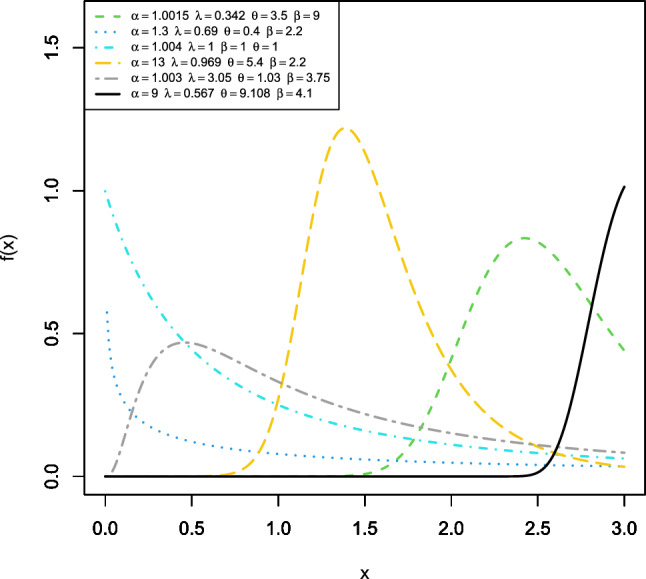
The shapes of the EAPLL PDF for different parameter combinations.

Figure 2.

The shapes of the EAPLL HRF for different parameter combinations.

Mathematical properties

In this section, we derived various properties of the EAPLL distribution, which include its linear representation, quantile function (QF), moments, and order statistics.

Useful expansion

In this section, the EAPLL density can be expressed as a linear mixture of exponentiated LL (ELL) densities.

Using the binomial expansion, we can write

$$\begin{array}{c}\hfill {\left[{\alpha }^{\frac{{(\lambda x)}^{\theta }}{1+{(\lambda x)}^{\theta }}},-,1\right]}^{\beta -1}=\sum _{k=0}^{\infty }{(-1)}^k\left(\begin{array}{c}\beta -1\\ k\end{array}\right){\left[{\alpha }^{\frac{{(\lambda x)}^{\theta }}{1+{\left(\lambda ,x\right)}^{\theta }}}\right]}^{\beta -k-1}.\end{array}$$ 6

The EAPLL PDF can be expressed as

$$\begin{array}{c}\hfill f_{\mathit{EAPLL}}(x;\mathrm{\Psi })=\sum _{k=0}^{\infty }{(-1)}^k\left(\begin{array}{c}\beta -1\\ k\end{array}\right)\frac{\beta \lambda \theta log(\alpha ){(\lambda x)}^{\theta -1}}{{(\alpha -1)}^{\beta }{\left[1,+,{(\lambda x)}^{\theta }\right]}^2}{\left[{\alpha }^{\frac{{(\lambda x)}^{\theta }}{1+{(\lambda x)}^{\theta }}}\right]}^{\beta -k}.\end{array}$$ 7

Using power series for the last term of Eq. (7), we obtain

$$\begin{array}{c}\hfill {\left[{\alpha }^{\frac{{(\lambda x)}^{\theta }}{1+{(\lambda x)}^{\theta }}}\right]}^{\beta -k}=\sum _{j=0}^{\infty }\frac{{(\beta -k)}^j}{j!}{\left(log,\alpha \right)}^j{\left[\frac{{(\lambda x)}^{\theta }}{1+{\left(\lambda ,x\right)}^{\theta }}\right]}^j.\end{array}$$ 8

Therefore Eq. (7) becomes

$$\begin{array}{c}\hfill f_{\text{EAPLL}}(x;\mathrm{\Psi })=\sum _{k,j=0}^{\infty }{(-1)}^k\left(\begin{array}{c}\beta -1\\ k\end{array}\right){(\beta -k)}^j\frac{\beta {(log\alpha )}^{j+1}}{{(\alpha -1)}^{\beta }j!}\frac{\lambda \theta {(\lambda x)}^{\theta (j+1)-1}}{{\left[1,+,{(\lambda x)}^{\theta }\right]}^{j+2}}.\end{array}$$ 9

Hence, the EAPLL density is reduced to

$$\begin{array}{c}\hfill f_{\text{EAPLL}}(x)=\sum _{j=0}^{\infty }{c}_j{z}_{\theta \left(j,+,1\right)}(x),\end{array}$$ 10

where

$$\begin{array}{c}\hfill c_j=\sum _{k=0}^{\infty }\frac{{(-1)}^k}{j+1}\left(\begin{array}{c}\beta -1\\ k\end{array}\right){(\beta -k)}^j\frac{\beta {(log\alpha )}^{j+1}}{{(\alpha -1)}^{\beta }j!}\end{array}$$ 11

and $z_{\theta (j+1)}(x)$ is the ELL density function with power parameter $(j+1)$. Equation (11) indicates that the EAPLL PDF is a linear combination of the ELL distribution and hence, some of its properties can be derived from those of the ELL distribution.

Quantile function

By utilizing the inverse transformation method, the QF can be obtained by inverting the CDF of the EAPLL distribution.

The QF of the EAPLL distribution follows as

$$\begin{array}{c}\hfill Q_x(p)=\frac{1}{\lambda }{\left\{\frac{ln\left[p^{1/\beta },(\alpha -1),+,1\right]}{ln\alpha -ln\left[p^{1/\beta },(\alpha -1),+,1\right]}\right\}}^{\frac{1}{\theta }},0<p<1.\end{array}$$ 12

The QF is useful in the simulation of random variables from the EAPLL distribution and in getting quartiles, skewness, and kurtosis. Table 1 gives numerical values of the EAPLL QF for some parameter combinations.

Table 1.

Some values of the EAPLL QF for different parameter combinations $(\beta ,\lambda ,\theta ,\alpha )$.

p	0.1	0.2	0.3	0.4	0.5	0.6	0.7	0.8	0.9
(1.2,10,1.9,0.05)	0.008	0.016	0.026	0.037	0.050	0.066	0.087	0.116	0.165
(0.1,1.2,1.1,1.05)	0.483	1.023	1.636	2.343	3.179	4.202	5.522	7.381	10.560
(0.5,7,0.5,1.1)	0.028	0.060	0.096	0.137	0.186	0.245	0.323	0.431	0.617
(0.1,1.3,1.05,1.1)	0.494	1.046	1.671	2.394	3.248	4.294	5.642	7.542	10.790
(1.3,7,1.1,2.1)	0.010	0.020	0.032	0.046	0.063	0.083	0.109	0.146	0.209
(1.2,10,1.9,1.05)	0.390	0.189	0.109	0.066	0.041	0.024	0.013	0.006	0.002
(0.5,1,5,1.1)	5460.352	396.053	81.188	24.685	9.015	3.549	1.385	0.479	0.111
(1,10,1.1,1.05)	0.084	0.039	0.021	0.012	0.007	0.004	0.002	0.001	0.000
(0.1,1,1.01,1.1)	0.505	0.061	0.009	0.001	0.000	0.000	0.000	0.000	0.000
(1.1,1,2.01,1.1)	2444.340	221.640	51.128	16.751	6.439	2.629	1.052	0.370	0.086
(2.1,2,1.01,1.1)	36.384	9.371	3.775	1.785	0.897	0.452	0.215	0.088	0.024
(2,1,1.01,1.1)	1440.694	150.545	37.391	12.831	5.089	2.124	0.863	0.306	0.071

The Galton’s skewness and Moors’ kurtosis are preferred as they are less sensitive to outliers. They are also known to exist even if distributions have no moments.

Galton’s skewness (also called Bowley’s skewness) is given as

$$\begin{array}{c}\hfill G=\frac{Q\left(\frac{3}{4}\right)+Q\left(\frac{1}{4}\right)-2Q\left(\frac{1}{2}\right)}{Q\left(\frac{3}{4}\right)-Q\left(\frac{1}{4}\right)}.\end{array}$$ 13

The Moors’ kurtosis³¹ is given as

$$\begin{array}{c}\hfill M=\frac{Q\left(\frac{3}{8}\right)-Q\left(\frac{1}{8}\right)+Q\left(\frac{7}{8}\right)-Q\left(\frac{5}{8}\right)}{Q\left(\frac{6}{8}\right)-Q\left(\frac{2}{8}\right)}.\end{array}$$ 14

Figure 3 illustrates the variation of Moors’ kurtosis for different values of the parameter $\beta$, where the additional shape parameter influences the kurtosis of the EAPLL distribution. Moreover, Fig. 4 shows the plots of Bowley’s skewness. It indicates that the skewness of the EAPLL distribution is affected by the extra shape parameter. It is noted that the increasing of $\beta$ for fixed values of $\alpha ,\theta$ and $\lambda$, increases both the values of skewness and kurtosis indicating asymmetry and heavy tails in the distribution.

Figure 3.

Plots of Moors’ kurtosis for the EAPLL distribution with fixed values of $\alpha =0.015$, $\theta =0.37$, and $\lambda =1.75$.

Figure 4.

Plots of Galton skewness for the EAPLL distribution with fixed values of $\alpha =0.015$, $\theta =0.37$, and $\lambda =1.75$.

Moments

The rth raw moment of the EAPLL distribution is defined as

$$\begin{array}{c}\hfill \begin{array}{cc}\hfill {\mu }_r^{\prime }& =E\left(X^r\right)\hfill \\ \hfill & ={\int }_0^{\infty }{x}^r{f}_{\mathit{EAPLL}}(x)dx\hfill \\ \hfill & ={\int }_0^{\infty }{x}^r\frac{\beta \theta \lambda }{{(\alpha -1)}^{\beta }}\frac{log(\alpha )}{{\left[1,+,{\left(\lambda ,x\right)}^{\theta }\right]}^2}{\left(\lambda ,x\right)}^{\theta -1}{\alpha }^{\frac{{\left({\lambda }_x\right)}^{\theta }}{1+{\left(\lambda ,x\right)}^{\theta }}}{\left({\alpha }^{\frac{{\left(\lambda ,x\right)}^{\theta }}{1+{\left(\lambda ,x\right)}^{\theta }}},-,1\right)}^{\beta -1}dx\hfill \\ \hfill & =\sum _{j=0}^{\infty }{c}_j{\int }_0^{\infty }{x}^r\lambda \theta (j+1)\frac{{(\lambda x)}^{\theta (j+1)-1}}{{\left[1,+,{(\lambda x)}^{\theta }\right]}^{j+2}}dx\hfill \\ \hfill & =\theta \lambda \sum _{j=0}^{\infty }{c}_j(j+1){\int }_0^{\infty }{x}^r\frac{{(\lambda x)}^{\theta (j+1)-1}}{{\left[1,+,{(\lambda x)}^{\theta }\right]}^{j+2}}dx,\hfill \end{array}\end{array}$$ 15

Let $u={(\lambda x)}^{\theta }$ and substituting into Eq. (15), we obtain

$$\begin{array}{c}\hfill \begin{array}{c}\hfill {\mu }_r^{\prime }=\sum _{j=0}^{\infty }{c}_j\frac{j+1}{{\lambda }^r}{\int }_0^{\infty }\frac{u^{\frac{r}{\theta }+j}}{{(1+u)}^{j+2}}du.\end{array}\end{array}$$ 16

Hence, for the EAPLL model can be written, in terms of beta function, as

$$\begin{array}{c}\hfill \begin{array}{c}\hfill {\mu }_r^{\prime }=\sum _{j=0}^{\infty }{c}_j\frac{j+1}{{\lambda }^r}B\left(\frac{r}{\theta },+,j,+,1,,,1,-,\frac{r}{\theta }\right),\end{array}\end{array}$$ 17

where $c_j$ is defined in Eq. (11).

Table 2 presents a summary of moments of the EAPLL distribution for various combinations of $\beta$, $\lambda$, $\theta$, and $\alpha$. The moments listed in the table include the first five raw moments, standard deviation (SD), coefficient of variation (CV), coefficient of skewness (CS), and coefficient of kurtosis (CK). These moments aid in the understanding and characterization of the EAPLL distribution under various scenarios. Across the various combinations of $\beta$, $\lambda$, $\theta$, and $\alpha$, we observe notable differences in the moments. For instance, by adjusting the parameter values, we observe a corresponding change in the SD indicating a change in variability in the distribution. Additionally, for various parameter combinations, we observe asymmetry in the EAPLL distribution.

Table 2.

A summary of moments of the EAPLL distribution for different parameter combinations $(\beta ,\lambda ,\theta ,\alpha )$.

$\beta$	$\lambda$	$\theta$	$\alpha$	${\mu }_1^{\prime }$	${\mu }_2^{\prime }$	${\mu }_3^{\prime }$	${\mu }_4^{\prime }$	${\mu }_5^{\prime }$	SD	CV	CS	CK
0.98	1	0.6	0.57	0.0723	0.0481	0.0360	0.0288	0.0239	0.2071	2.8648	2.9628	10.7386
	1	0.6	4.75	0.2054	0.1280	0.0927	0.0726	0.0596	0.2928	1.4254	1.2410	3.1952
	1	1	0.57	0.0714	0.0481	0.0362	0.0290	0.0242	0.2073	2.9037	2.9873	10.8569
	3	0.6	0.57	0.5220	0.3245	0.2341	0.1827	0.1497	0.2283	0.4373	0.8645	0.6740
	3	0.6	4.75	0.0669	0.0419	0.0304	0.0237	0.0195	0.1935	2.8942	3.1116	11.9081
1.1	1	0.95	4.25	0.4592	0.3116	0.2354	0.1891	0.1580	0.3173	0.6910	−0.0034	1.7216
	1	0.99	4.75	0.4849	0.3316	0.2516	0.2026	0.1695	0.3105	0.6404	−0.0906	1.7775
	1	0.95	4.75	0.5108	0.3468	0.2622	0.2107	0.1760	0.2931	0.5739	−0.1089	1.8529
	1	1	4.72	0.4750	0.3253	0.2470	0.1990	0.1666	0.3157	0.6647	−0.0689	1.7438
	1	1	4	0.4775	0.3270	0.2484	0.2001	0.1675	0.3147	0.6590	−0.0761	1.7514
1.8	7	0.6	2.75	0.0728	0.0394	0.0264	0.0197	0.0157	0.1847	2.5370	2.9507	11.3585
	7	0.6	0.57	0.0108	0.0056	0.0036	0.0027	0.0021	0.0738	6.8454	8.6215	85.3383
	7	1	2.75	0.2558	0.1710	0.1280	0.1021	0.0848	0.3250	1.2703	0.8793	2.2813
	7	1	0.57	0.0188	0.0105	0.0071	0.0054	0.0043	0.1007	5.3600	6.4319	47.3815

Order statistics

Consider the order statistics of a random sample from the EAPLL distribution, denoted by

$x_{1:n},x_{2:n},...,x_{n:n}$. The PDF of the ith order statistic is given as

$$\begin{array}{c}\hfill f_{X_{i:n}}(x)=\frac{1}{B(i,n-i+1)}f(x)\sum _{p=0}^{n-i}{(-1)}^p\left(\begin{array}{c}n-i\\ p\end{array}\right)F{(x)}^{p+i-1}.\end{array}$$ 18

By utilizing the generalized binomial expansion and the power series, we get

$$\begin{array}{c}\hfill F{(x)}^{p+i-1}=\omega \sum _{q=0}^{\beta (p+i-1)}\sum _{m=0}^{\infty }{(-1)}^q\left(\begin{array}{c}\beta (p+i-1)\\ q\end{array}\right){(\beta (p+i-1)-q)}^m\frac{{(log\alpha )}^m}{m!}\frac{{(\lambda x)}^{\theta m}}{{\left[1,+,{(\lambda x)}^{\theta }\right]}^m},\end{array}$$ 19

Hence, we can write

$$\begin{array}{cc}\hfill f(x)F{(x)}^{p+i-1}=& \omega \sum _{q,m,k,j=0}^{\infty }{(-1)}^{k+q}\left(\begin{array}{c}\beta -1\\ k\end{array}\right){(\beta -k)}^j\frac{\beta \lambda \theta }{{(\alpha -1)}^{\beta }j!}\hfill \\ \hfill & \frac{{(\lambda x)}^{\theta (m+j+1)-1}}{{\left[1,+,{(\lambda x)}^{\theta }\right]}^{m+j+2}}\times \left(\begin{array}{c}\beta (p+i-1)\\ q\end{array}\right){(\beta (p+i-1)-q)}^m\frac{{(log\alpha )}^{j+m+1}}{m!}.\hfill \end{array}$$ 20

Combining the last equation with Eq. (18), we obtain

$$\begin{array}{c}\hfill f_{Xi:n}=\sum _{m=0}^{\infty }{d}_m{t}_{(m+j+1),\lambda ,\theta }(x),\end{array}$$ 21

where

$$\begin{array}{c}\hfill \begin{array}{cc}\hfill d_m=& \omega \sum _{q,k,j=0}^{\infty }{(-1)}^{k+q}\left(\begin{array}{c}\beta -1\\ k\end{array}\right){(\beta -k)}^j\frac{\beta {(\beta (p+i-1)-q)}^m}{(m+j+1){(\alpha -1)}^{\beta }}\left(\begin{array}{c}\beta (p+i-1)\\ q\end{array}\right)\frac{{(log\alpha )}^{j+m+1}}{m!j!}\hfill \end{array}\end{array}$$ 22

and $\omega ={(\alpha -1)}^{-\beta (p+i-1)}$. and $t_{(m+j+1),\lambda ,\theta }(x)$ denotes the ELL density with power parameter $(m+j+1)$. Consequently, the PDF of the EAPLL order statistics can be expressed as a linear combination of the ELL densities. Based on Eq. (21), some structural characteristics of $X_{i:n}$ can be obtained from those ELL properties.

Parameter estimation

The existing extensions of the LL distribution in the literature rely on a single estimation method. This might fall short of enhancing parameter estimation accuracy. Consequently, in this section, we explore eight different classical estimation methods to estimate the EAPLL parameters called the maximum likelihood estimators (MLEs), maximum product of spacing estimators (MPSEs), ordinary least-squares estimators (OLSEs), weighted least-squares estimators (WLSEs), Anderson–Darling estimators (ADEs), Cramér–von Mises estimators (CVMEs), percentiles estimators (PCEs), and right-tail ADEs (RADEs). To improve the clarity of the estimation methods, we have included a more detailed context for each equation, explaining how they are derived. This enhancement aims to provide a comprehensive understanding of the estimation techniques, making the section more informative and accessible to readers.

Maximum likelihood

In this subsection, the maximum likelihood (ML) approach is employed to estimate the EAPLL parameters. Hence, the log-likelihood function reduces to

$$\begin{array}{cc}\hfill \ell (x\mid \beta ,\alpha ,\lambda ,\theta )=& nlog(\beta \lambda \theta )+(\theta -1)\sum _{i=1}^{n}log\left(\lambda ,x_i\right)+nlog(log\alpha )+\sum _{i=1}^n\left(\frac{{\left(\lambda ,x_i\right)}^{\theta }}{1+{\left(\lambda ,x_i\right)}^{\theta }}\right)log\alpha \hfill \\ \hfill & +(\beta -1)\sum _{i=1}^{n}log\left({\eta }_i,-,1\right)-n\beta log(\alpha -1)-2nlog\left[1,+,{\left(\lambda ,x_i\right)}^{\theta }\right],\hfill \end{array}$$ 23

where ${\eta }_i={\alpha }^{\frac{{(\lambda x_i)}^{\theta }}{1+{(\lambda x_i)}^{\theta }}}.$

The score functions are derived by taking the first partial derivatives of the log-likelihood function with respect to $\alpha ,\beta ,\lambda$ and $\theta$ as indicated below.

$$\begin{array}{cc}\hfill & \frac{\partial \ell }{\partial \beta }=\frac{n}{\beta }-nlog(\alpha -1)+\sum _{i=1}^{n}log\left({\eta }_i,-,1\right),\hfill \end{array}$$ 24

$$\begin{array}{cc}\hfill & \frac{\partial \ell }{\partial \theta }=\frac{n}{\theta }+\sum _{i=1}^{n}log\left(\lambda ,x_i\right)-\sum _{i=1}^n\frac{{(\lambda x_i)}^{\theta }log(\lambda x_i)log\alpha }{{\left[1,+,{(\lambda x_i)}^{\theta }\right]}^2}+(1-\beta )\sum _{i=1}^n\frac{{(\lambda x_i)}^{\theta }log(\lambda x_i)(log\alpha ){\eta }_i}{\left({\eta }_i,-,1\right){\left[1,+,{(\lambda x_i)}^{\theta }\right]}^2},\hfill \end{array}$$ 25

$$\begin{array}{cc}\hfill & \frac{\partial \ell }{\partial \lambda }=\frac{n}{\lambda }+\frac{n(\theta -1)}{\lambda }+\sum _{i=1}^n\frac{\theta {(\lambda x_i)}^{\theta }log\alpha }{\lambda {\left[1,+,{(\lambda x_i)}^{\theta }\right]}^2}+(1-\beta )\sum _{i=1}^n\frac{\theta {(\lambda x_i)}^{\theta }(log\alpha ){\eta }_i}{\lambda {\left[1,+,{(\lambda x_i)}^{\theta }\right]}^2\left({\eta }_i,-,1\right)}-\frac{2n\theta {(\lambda x_i)}^{\theta }}{\lambda \left[1,+,{(\lambda x_i)}^{\theta }\right]}\hfill \end{array}$$ 26

and

$$\begin{array}{c}\hfill \frac{\partial \ell }{\partial \alpha }=\frac{n}{\alpha log\alpha }+\sum _{i=1}^n\frac{{(\lambda x_i)}^{\theta }}{\alpha \left[1,+,{\left(\lambda ,x_i\right)}^{\theta }\right]}-\frac{n\beta }{\alpha -1}+(\beta -1)\sum _{i=1}^n\frac{{(\lambda x_i)}^{\theta }{\eta }_i}{\alpha \left[1,+,{(\lambda x_i)}^{\theta }\right]\left({\eta }_i,-,1\right)}.\end{array}$$ 27

The MLEs of the EAPLL parameters are obtained by equating the score functions to zero and solving the resulting system of equations. Since the score functions do not exist in closed form, numerical methods may be applied to solve them. This study has utilized the algorithm of the Broyden–Fletcher–Goldfarb–Shanno (BFGS) method for solving this non-linear system of equations.

Maximum product of spacing

The maximum product of spacing (MPS) method is used to estimate the parameters of continuous univariate models as an alternative to the ML method. The uniform spacings of a random sample of size n from the EAPLL distribution are defined by

$$\begin{array}{c}\hfill B_{i:n}(\beta ,\lambda ,\theta ,\alpha )=F(x_{i:n})-F(x_{i-1:n}),\end{array}$$ 28

where $F(x_{0:n})=0$, $F(x_{n+1:n})=1$ and ${\sum }_{i=0}^{n+1}{B}_{i:n}(\beta ,\lambda ,\theta ,\alpha )=1$.

Consider the order statistics of a random sample from the EAPLL distribution, denoted by $x_{1:n},x_{2:n},...,x_{n:n}$. Then, the MPSEs of the EAPLL parameters are obtained by maximizing the following function

$$\begin{array}{c}\hfill D(\beta ,\lambda ,\theta ,\alpha )=\frac{1}{n+1}\sum _{i=1}^{n+1}log{B}_{i:n}(\beta ,\lambda ,\theta ,\alpha ),\end{array}$$ 29

with respect to the parameters $\beta$, $\lambda$, $\theta$ and $\alpha$. Additionally, the MPSEs of the EAPLL parameters can be obtained by solving the following equations

$$\begin{array}{c}\hfill \frac{1}{n+1}\sum _{i=1}^{n+1}\frac{1}{B_{i:n}(\beta ,\lambda ,\theta ,\alpha )}\left({\delta }_r,(x_{i:n}|\beta ,\lambda ,\theta ,\alpha ),-,{\delta }_r,(x_{i-1:n}|\beta ,\lambda ,\theta ,\alpha )\right)=0,r=1,2,3,4,\end{array}$$ 30

where

$$\begin{array}{cc}\hfill & \begin{array}{c}\hfill {\delta }_1(x_{i:n}|\beta ,\lambda ,\theta ,\alpha )=\frac{\partial }{\partial \beta }F(x_{i:n})={\left(\frac{{\eta }_{i:n}-1}{\alpha -1}\right)}^{\beta }log\left(\frac{{\eta }_{i-1:n}}{\alpha -1}\right),\end{array}\hfill \end{array}$$ 31

$$\begin{array}{cc}\hfill & \begin{array}{c}\hfill {\delta }_2(x_{i:n}|\beta ,\lambda ,\theta ,\alpha )=\frac{\partial }{\partial \lambda }F(x_{i:n})=\frac{\beta \theta {\eta }_{i:n}{x}_{i:n}(log\alpha ){({\eta }_{i:n}-1)}^{\beta -1}{(\lambda x_{i:n})}^{\theta -1}}{{(\alpha -1)}^{\beta }{\left[1,+,{(\lambda x_{i:n})}^{\theta }\right]}^2},\end{array}\hfill \end{array}$$ 32

$$\begin{array}{cc}\hfill & \begin{array}{c}\hfill {\delta }_3(x_{i:n}|\beta ,\lambda ,\theta ,\alpha )=\frac{\partial }{\partial \theta }F(x_{i:n})=\frac{\beta {\eta }_{i:n}(log\alpha ){({\eta }_{i:n}-1)}^{\beta -1}{(\lambda x_{i:n})}^{\theta }(log(\lambda x_{i:n}))}{{(\alpha -1)}^{\beta }{\left[1,+,{(\lambda x_{i:n})}^{\theta }\right]}^2}\end{array}\hfill \end{array}$$ 33

and

$$\begin{array}{c}\hfill \begin{array}{c}\hfill {\delta }_4(x_{i:n}|\beta ,\lambda ,\theta ,\alpha )=\frac{\partial }{\partial \alpha }F(x_{i:n})=\beta {\left(\frac{{\eta }_{i-1:n}}{\alpha -1}\right)}^{\beta -1}\left[\frac{{(\lambda x_{i:n})}^{\theta }(\alpha -{\eta }_{i:n})-\alpha (1-{\eta }_{i:n})}{\alpha {(\alpha -1)}^2\left[1,+,{(\lambda x_{i:n})}^{\theta }\right]}\right],\end{array}\end{array}$$ 34

where ${\eta }_{i:n}={\alpha }^{\frac{{(\lambda x_{i:n})}^{\theta }}{1+{(\lambda x_{i:n})}^{\theta }}}.$

Ordinary and weighted least-squares

The OLSEs of the unknown parameters of the EAPLL distribution are obtained by minimizing the following function

$$\begin{array}{c}\hfill OL=\sum _{i=1}^n{\left[F,\left(x_{i:n}\right),-,\frac{i}{n+1}\right]}^2.\end{array}$$ 35

Substituting the EAPLL CDF into the above equation yields

$$\begin{array}{c}\hfill OL=\sum _{i=1}^n{\left[{\left(\frac{{\eta }_{i:n}-1}{\alpha -1}\right)}^{\beta },-,\frac{i}{n+1}\right]}^2.\end{array}$$ 36

Furthermore, the OLSEs of the EAPLL parameters can be obtained by solving the following system of non-linear equations (for $r=1,2,3,4$)

$$\begin{array}{c}\hfill \sum _{i=1}^n\left[{\left(\frac{{\eta }_{i:n}-1}{\alpha -1}\right)}^{\beta },-,\frac{i}{n+1}\right]{\delta }_r(x_{i:n}|\beta ,\lambda ,\theta ,\alpha )=0,\end{array}$$ 37

where ${\delta }_r(x_{i:n}|\beta ,\lambda ,\theta ,\alpha )$ are defined in Eqs. (31)–(34) for $r=1,2,3,4$.

The WLSEs of the EAPLL parameters can be calculated by minimizing the following function

$$\begin{array}{c}\hfill W=\sum _{i=1}^n\frac{{(n+1)}^2(n+2)}{i(n-i+1)}{\left[{\left(\frac{{\eta }_{i:n}-1}{\alpha -1}\right)}^{\beta },-,\frac{i}{n+1}\right]}^2.\end{array}$$ 38

Furthermore, the WLSEs of the EAPLL parameters can also be obtained by solving the following system of non-linear equations (for r=1,2,3,4,)

$$\begin{array}{c}\hfill \sum _{i=1}^n\frac{{(n+1)}^2(n+2)}{i(n-i+1)}\left[{\left(\frac{{\eta }_{i:n}-1}{\alpha -1}\right)}^{\beta },-,\frac{i}{n+1}\right]{\delta }_r(x_{i:n}|\beta ,\lambda ,\theta ,\alpha )=0.\end{array}$$ 39

Anderson–Darling and right-tail Anderson–Darling

The Anderson–Darling (AD) method is used to estimate the parameters of any distribution based on observed data. Specifically, it measures the discrepancy between the observed data and the hypothesized distribution. It takes into account both the proximity of the data points to the theoretical distribution and the importance of the tails of the distribution. The ADEs belong to the category of minimum distance estimators.

To obtain the ADEs of the EAPLL parameters, one can minimize the following equation with respect to $\beta ,\lambda ,\theta$ and $\alpha$:

$$\begin{array}{c}\hfill A-D=-n-\frac{1}{n}\sum _{i=1}^n(2i-1)\left\{log,[F(x_{i:n})],+,log,[S(x_{n+1-i:n})]\right\}.\end{array}$$ 40

Correspondingly, the ADEs for the EAPLL parameters are also obtained by solving the following system of non-linear equations (for $r,k=1,2,3,4$)

$$\begin{array}{c}\hfill \sum _{i=1}^n\left(\frac{{\delta }_r(x_{i:n}|\beta ,\lambda ,\theta ,\alpha )}{F(x_{i:n})},-,\frac{{\delta }_k(x_{n+1-i:n}|\beta ,\lambda ,\theta ,\alpha )}{S(x_{n+1-i:n})}\right)=0.\end{array}$$ 41

The RADEs of the EAPLL parameters are obtained by minimizing the function

$$\begin{array}{c}\hfill RA=\frac{n}{2}-2\sum _{i=1}^{n}F\left(x_{i:n}\right)-\frac{1}{n}\sum _{i=1}^n(2i-1)log\left[S,\left(x_{n+1-i:n}\right)\right].\end{array}$$ 42

The RADEs are also determined by solving the system of non-linear equations (for r=1,2,3,4)

$$\begin{array}{c}\hfill -2\sum _{i=1}^n{\delta }_r\left(x_{i:n}\right)+\frac{1}{n}\sum _{i=1}^n(2i-1)\frac{{\delta }_r\left(x_{n+1-i:n}\right)}{S\left(x_{n+1-i:n}\right)}=0.\end{array}$$ 43

Cramér–von Mises and percentiles

The CVMEs belong to the minimum distance estimators and they exhibit less bias as compared to other estimators of the same type. These estimators can be derived by computing the difference between the estimated CDF and the empirical CDF. To obtain the CVMEs of the EAPLL parameters, one can minimize the following equation with respect to $\beta ,\lambda ,\theta$ and $\alpha$:

$$\begin{array}{c}\hfill CV=\frac{1}{12n}+\sum _{i=1}^n{\left[{\left(\frac{{\eta }_{i:n}-1}{\alpha -1}\right)}^{\beta },-,\left(\frac{2i-1}{2n}\right)\right]}^2.\end{array}$$ 44

Likewise, the CVMEs can also be determined by solving the following system of non-linear equations

(for $r=1,2,3,4$)

$$\begin{array}{c}\hfill \sum _{i=1}^n\left[{\left(\frac{{\eta }_{i:n}-1}{\alpha -1}\right)}^{\beta },-,\left(\frac{2i-1}{2n}\right)\right]{\delta }_r(x_{i:n}|\beta ,\lambda ,\theta ,\alpha )=0,\end{array}$$ 45

where ${\delta }_r(x_{i:n}|\beta ,\lambda ,\theta ,\alpha )$ are defined in Eqs. (31)–(34) for $r=1,2,3,4$.

Consider an unbiased estimator $p_i=i/(1+n)$ of $F(x_{i:n})$. Then, the PCEs of the EAPLL parameters are obtained by minimizing the function

$$\begin{array}{c}\hfill P(\beta ,\lambda ,\theta ,\alpha )=\sum _{i=1}^n{\left(x_{i:n},-,\frac{1}{\lambda },{\left\{\frac{ln\left[p_i^{1/\beta },(\alpha -1),+,1\right]}{ln\alpha -ln\left[p_i^{1/\beta },(\alpha -1),+,1\right]}\right\}}^{1/\theta }\right)}^2,\end{array}$$ 46

with respect to the parameters $\beta ,\lambda ,\theta$ and $\alpha$.

Monte Carlo simulations

In this section, an extensive simulation study is conducted to explore the performance of different estimators of the EAPLL distribution parameters. Using the QF (12), we generate random samples of sizes $n=(20,50,100,300,500)$ from the EAPLL distribution. The simulations are replicated $N=2000$ times for each sample size and the corresponding results are obtained for different parameter combinations, where $\beta =(1.8,2.72),\lambda =(0.75,0.8),\theta =(0.6,1)$ and $\alpha =(1.57,2.75)$. The choice of initial parameter values in the simulation study was guided by the desire to capture and imitate real-world scenarios, with a focus on individual variations and the use of real-world data. This approach was taken to ensure the validity and reliability of the results, as well as to facilitate reproducibility and the use of pseudo-random number generators in the simulation process.

The numerical results are obtained using nlminb() function in R software. Furthermore, the average values of the estimates (AEs), absolute average bias (ABs), and mean square errors (MSEs) of the estimates are determined and presented in Tables 3, 4, 5, 6, 7, 8, 9 and 10.

Table 3.

Simulation results of eight different estimators for $\beta =1.8,\lambda =0.75,\theta =0.6,\alpha =1.57$.

n	Measures	Parameters	MLEs	MPSEs	OLSEs	WLSEs	ADEs	CVMEs	PCEs	RADEs
20	AEs	$\beta$	$2.{09746}^7$	$1.{78359}^6$	$1.{71928}^4$	$1.{36221}^2$	$1.{42514}^3$	$1.{77951}^5$	$1.{21904}^1$	$2.{20069}^8$
		$\lambda$	$1.{30780}^8$	$0.{83407}^4$	$0.{58000}^2$	$1.{27839}^7$	$1.{24909}^5$	$0.{79788}^3$	$0.{44958}^1$	$1.{25369}^6$
		$\theta$	$0.{64299}^7$	$0.{56072}^1$	$1.{58000}^8$	$0.{57783}^2$	$0.{61660}^5$	$0.{63314}^6$	$0.{59385}^3$	$0.{61482}^4$
	MSEs	$\alpha$	$1.{00004}^1$	$1.{56748}^8$	$1.{00017}^2$	$1.{01227}^5$	$1.{00537}^4$	$1.{53722}^7$	$1.{49703}^6$	$1.{00022}^3$
		$\beta$	$0.{63984}^2$	$0.{64000}^5$	$0.{64000}^5$	$0.{64000}^5$	$0.{64000}^5$	$0.{64000}^5$	$0.{38321}^1$	$2.{56222}^8$
		$\lambda$	$0.{45529}^4$	$0.{38809}^1$	$0.{40314}^3$	$0.{45824}^6$	$0.{45615}^5$	$0.{40266}^2$	$0.{87720}^7$	$0.{96407}^8$
		$\theta$	$0.{00835}^2$	$0.{01008}^3$	$0.{01043}^4$	$0.{01100}^5$	$0.{00806}^1$	$0.{01193}^6$	$0.{06674}^8$	$0.{02247}^7$
	ABs	$\alpha$	$0.{32490}^{5.5}$	$0.{07911}^1$	$0.{15864}^3$	$0.{32489}^4$	$0.{32490}^{5.5}$	$0.{15409}^2$	$0.{51727}^7$	$0.{80459}^8$
		$\beta$	$0.{79990}^2$	$0.{80000}^5$	$0.{80000}^5$	$0.{80000}^5$	$0.{80000}^5$	$0.{80000}^5$	$0.{61904}^1$	$1.{60069}^8$
		$\lambda$	$0.{67475}^4$	$0.{62297}^1$	$0.{63494}^3$	$0.{67694}^6$	$0.{67539}^5$	$0.{63455}^2$	$0.{93659}^7$	$0.{98187}^8$
		$\theta$	$0.{09136}^2$	$0.{10038}^3$	$0.{10215}^4$	$0.{10490}^5$	$0.{08976}^1$	$0.{10924}^6$	$0.{25834}^8$	$0.{14991}^7$
	$\sum Ranks$	$\alpha$	$0.{57000}^{5.5}$	$0.{28127}^1$	$0.{39830}^3$	$0.{56999}^4$	$0.{57000}^{5.5}$	$0.{39254}^2$	$0.{71921}^7$	$0.{89699}^8$
			${50}^{3.5}$	${39}^1$	${46}^2$	${56}^6$	${50}^{3.5}$	${51}^5$	${61}^7$	${83}^8$
50	AEs	$\beta$	$1.{80585}^7$	$1.{73494}^4$	$1.{80285}^6$	$1.{49615}^3$	$1.{44570}^2$	$1.{78379}^5$	$1.{14991}^1$	$1.{87590}^8$
		$\lambda$	$1.{31902}^8$	$0.{74899}^2$	$0.{95478}^4$	$1.{10741}^5$	$1.{26827}^7$	$0.{88721}^3$	$0.{40490}^1$	$1.{09852}^6$
		$\theta$	$0.{61093}^6$	$0.{58263}^1$	$0.{59294}^3$	$0.{59671}^4$	$0.{61245}^8$	$0.{61239}^7$	$0.{58768}^2$	$0.{60750}^5$
	MSEs	$\alpha$	$1.{00066}^1$	$1.{57887}^8$	$1.{36249}^6$	$1.{02458}^3$	$1.{04555}^4$	$1.{29198}^5$	$1.{41052}^7$	$1.{00092}^2$
		$\beta$	$0.{63984}^3$	$0.{55165}^2$	$0.{64000}^{5.5}$	$0.{64000}^{5.5}$	$0.{64000}^{5.5}$	$0.{64000}^{5.5}$	$0.{34101}^1$	$1.{62809}^8$
		$\lambda$	$0.{41582}^5$	$0.{28695}^1$	$0.{37292}^2$	$0.{39218}^4$	$0.{41843}^6$	$0.{37641}^3$	$0.{88101}^8$	$0.{86812}^7$
		$\theta$	$0.{00383}^1$	$0.{00466}^3$	$0.{00596}^5$	$0.{00570}^4$	$0.{00430}^2$	$0.{00612}^6$	$0.{05837}^8$	$0.{00919}^7$
	ABs	$\alpha$	$0.{32490}^{5.5}$	$0.{04873}^1$	$0.{30435}^2$	$0.{32489}^4$	$0.{32490}^{5.5}$	$0.{31433}^3$	$0.{41104}^7$	$0.{44785}^8$
		$\beta$	$0.{79990}^3$	$0.{74273}^2$	$0.{80000}^{5.5}$	$0.{80000}^{5.5}$	$0.{80000}^{5.5}$	$0.{80000}^{5.5}$	$0.{58396}^1$	$1.{2759}^8$
		$\lambda$	$0.{64484}^5$	$0.{53568}^1$	$0.{61067}^2$	$0.{62624}^4$	$0.{64686}^6$	$0.{61352}^3$	$0.{93862}^8$	$0.{93173}^7$
		$\theta$	$0.{06188}^1$	$0.{06828}^3$	$0.{07723}^5$	$0.{07553}^4$	$0.{06557}^2$	$0.{07821}^6$	$0.{24161}^8$	$0.{09585}^7$
	$\sum Ranks$	$\alpha$	$0.{57000}^{5.5}$	$0.{22074}^1$	$0.{55168}^2$	$0.{56999}^4$	$0.{57000}^{5.5}$	$0.{56065}^3$	$0.{64112}^7$	$0.{66922}^8$
			${51}^4$	${29}^1$	${48}^2$	${50}^3$	${59}^{6.5}$	${55}^5$	${59}^{6.5}$	${81}^8$
100	AEs	$\beta$	$1.{77425}^8$	$1.{75071}^6$	$1.{65464}^4$	$1.{55109}^3$	$1.{42874}^2$	$1.{76222}^7$	$1.{11177}^1$	$1.{69885}^5$
		$\lambda$	$1.{25980}^7$	$0.{73063}^2$	$0.{98402}^3$	$1.{17632}^6$	$1.{32867}^8$	$0.{99105}^4$	$0.{50348}^1$	$1.{06644}^5$
		$\theta$	$0.{60018}^5$	$0.{59366}^3$	$0.{59909}^4$	$0.{59292}^2$	$0.{60205}^8$	$0.{60143}^6$	$0.{58040}^1$	$0.{60156}^7$
	MSEs	$\alpha$	$1.{00199}^1$	$1.{57961}^8$	$1.{28893}^6$	$1.{07731}^3$	$1.{12086}^4$	$1.{21141}^5$	$1.{36716}^7$	$1.{00556}^2$
		$\beta$	$0.{50490}^3$	$0.{28701}^1$	$0.{64000}^{5.5}$	$0.{64000}^{5.5}$	$0.{64000}^{5.5}$	$0.{64000}^{5.5}$	$0.{32576}^2$	$1.{20747}^8$
		$\lambda$	$0.{38041}^5$	$0.{19940}^1$	$0.{34738}^2$	$0.{37289}^4$	$0.{40140}^6$	$0.{35386}^3$	$0.{89047}^8$	$0.{72337}^7$
		$\theta$	$0.{00222}^1$	$0.{00250}^2$	$0.{00382}^5$	$0.{00315}^4$	$0.{00258}^3$	$0.{00420}^6$	$0.{04769}^8$	$0.{00450}^7$
	ABs	$\alpha$	$0.{32489}^6$	$0.{02916}^1$	$0.{32076}^4$	$0.{32481}^5$	$0.{32490}^7$	$0.{32064}^3$	$0.{38096}^8$	$0.{25413}^2$
		$\beta$	$0.{71057}^3$	$0.{53574}^1$	$0.{80000}^{5.5}$	$0.{80000}^{5.5}$	$0.{80000}^{5.5}$	$0.{80000}^{5.5}$	$0.{57075}^2$	$1.{09885}^8$
		$\lambda$	$0.{61677}^5$	$0.{44654}^1$	$0.{58939}^2$	$0.{61065}^4$	$0.{63356}^6$	$0.{59486}^3$	$0.{94364}^8$	$0.{85051}^7$
		$\theta$	$0.{04708}^1$	$0.{05001}^2$	$0.{06180}^5$	$0.{05615}^4$	$0.{05084}^3$	$0.{06481}^6$	$0.{21837}^8$	$0.{06709}^7$
	$\sum Ranks$	$\alpha$	$0.{56999}^6$	$0.{17078}^1$	$0.{56636}^4$	$0.{56992}^5$	$0.{57000}^7$	$0.{56625}^3$	$0.{61722}^8$	$0.{50411}^2$
			${51}^{3.5}$	${29}^1$	${50}^2$	${51}^{3.5}$	${65}^7$	${57}^5$	${62}^6$	${67}^8$
	AEs	$\beta$	$1.{65761}^5$	$1.{77057}^8$	$1.{66057}^6$	$1.{61653}^3$	$1.{50661}^2$	$1.{67375}^7$	$1.{00234}^1$	$1.{61819}^4$
		$\lambda$	$1.{11724}^6$	$0.{74471}^2$	$1.{02341}^5$	$0.{93275}^3$	$1.{13634}^7$	$1.{02224}^4$	$0.{56169}^1$	$1.{17334}^8$
		$\theta$	$0.{59272}^2$	$0.{59777}^5$	$0.{59516}^3$	$0.{59626}^4$	$0.{59825}^6$	$0.{60010}^8$	$0.{59249}^1$	$0.{59969}^7$
	MSEs	$\alpha$	$1.{06505}^1$	$1.{57213}^8$	$1.{31336}^7$	$1.{29559}^6$	$1.{20721}^3$	$1.{27060}^5$	$1.{26796}^4$	$1.{10575}^2$
		$\beta$	$0.{20521}^2$	$0.{08808}^1$	$0.{42990}^7$	$0.{22794}^3$	$0.{35183}^5$	$0.{41926}^6$	$0.{30386}^4$	$0.{52084}^8$
		$\lambda$	$0.{26541}^3$	$0.{06368}^1$	$0.{27543}^5$	$0.{22326}^2$	$0.{29660}^6$	$0.{26658}^4$	$0.{91692}^7$	$1.{03671}^8$
300		$\theta$	$0.{00104}^3$	$0.{00092}^1$	$0.{00167}^7$	$0.{00101}^2$	$0.{00109}^4$	$0.{00166}^6$	$0.{04669}^8$	$0.{00154}^5$
	ABs	$\alpha$	$0.{32476}^6$	$0.{00855}^1$	$0.{32249}^4$	$0.{32445}^5$	$0.{32490}^7$	$0.{32012}^3$	$0.{39760}^8$	$0.{08507}^2$
		$\beta$	$0.{45300}^2$	$0.{29678}^1$	$0.{65567}^7$	$0.{47743}^3$	$0.{59316}^5$	$0.{64750}^6$	$0.{55124}^4$	$1.{01819}^8$
		$\lambda$	$0.{51518}^3$	$0.{25235}^1$	$0.{52481}^5$	$0.{47250}^2$	$0.{54461}^6$	$0.{51632}^4$	$0.{65756}^7$	$0.{72169}^8$
		$\theta$	$0.{03227}^3$	$0.{03038}^1$	$0.{04083}^7$	$0.{03183}^2$	$0.{03299}^4$	$0.{04075}^6$	$0.{21607}^8$	$0.{03927}^5$
	$\sum Ranks$	$\alpha$	$0.{56988}^6$	$0.{09248}^1$	$0.{56788}^4$	$0.{56961}^5$	$0.{57000}^7$	$0.{56579}^3$	$0.{63055}^8$	$0.{29167}^2$
			${42}^3$	${31}^1$	${67}^{7.5}$	${40}^2$	${62}^{5.5}$	${62}^{5.5}$	${61}^4$	${67}^{7.5}$
500	AEs	$\beta$	$1.{67086}^7$	$1.{79009}^8$	$1.{62632}^4$	$1.{64936}^6$	$1.{55506}^2$	$1.{61795}^3$	$0.{84703}^1$	$1.{63722}^5$
		$\lambda$	$0.{90824}^4$	$0.{74903}^2$	$1.{04692}^7$	$0.{85683}^3$	$1.{15103}^8$	$0.{98194}^5$	$0.{49168}^1$	$1.{03080}^6$
		$\theta$	$0.{59329}^2$	$0.{59837}^7$	$0.{59707}^5$	$0.{59428}^4$	$0.{59376}^3$	$0.{60036}^8$	$0.{58603}^1$	$0.{59827}^6$
	MSEs	$\alpha$	$1.{12894}^2$	$1.{57046}^8$	$1.{35327}^6$	$1.{53839}^7$	$1.{20849}^3$	$1.{31855}^5$	$1.{06943}^1$	$1.{16244}^4$
		$\beta$	$0.{11403}^2$	$0.{00366}^1$	$0.{31584}^7$	$0.{12041}^3$	$0.{23957}^4$	$0.{29410}^5$	$0.{31004}^6$	$1.{07583}^8$
		$\lambda$	$0.{17897}^3$	$0.{00308}^1$	$0.{23841}^5$	$0.{15116}^2$	$0.{26813}^6$	$0.{22464}^4$	$0.{92226}^8$	$0.{40847}^7$
		$\theta$	$0.{00067}^3$	$0.{00049}^1$	$0.{00094}^6$	$0.{00061}^2$	$0.{00074}^4$	$0.{00099}^7$	$0.{04308}^8$	$0.{00092}^5$
	ABs	$\alpha$	$0.{32441}^5$	$0.{00048}^1$	$0.{32260}^4$	$0.{32447}^6$	$0.{32490}^7$	$0.{32182}^3$	$0.{38011}^8$	$0.{07641}^2$
		$\beta$	$0.{33768}^2$	$0.{06047}^1$	$0.{56200}^7$	$0.{34700}^3$	$0.{48946}^4$	$0.{54231}^5$	$0.{55681}^6$	$1.{03722}^8$
		$\lambda$	$0.{42305}^3$	$0.{05547}^1$	$0.{48828}^5$	$0.{38879}^2$	$0.{51781}^6$	$0.{47396}^4$	$0.{96034}^8$	$0.{63912}^7$
		$\theta$	$0.{02589}^3$	$0.{02207}^1$	$0.{03068}^6$	$0.{02478}^2$	$0.{02712}^4$	$0.{03148}^7$	$0.{20755}^8$	$0.{03036}^5$
	$\sum Ranks$	$\alpha$	$0.{56957}^5$	$0.{02198}^1$	$0.{56798}^4$	$0.{56962}^6$	$0.{57000}^7$	$0.{56729}^3$	$0.{61653}^8$	$0.{27642}^2$
			${41}^2$	${33}^1$	${66}^8$	${46}^3$	${58}^4$	${59}^5$	${64}^6$	${65}^7$

Table 4.

Simulation results of eight different estimators for $\beta =1.8,\lambda =0.75,\theta =0.6,\alpha =2.75$.

n	Measures	Parameters	MLEs	MPSEs	OLSEs	WLSEs	ADEs	CVMEs	PCEs	RADEs
20	AEs	$\beta$	$2.{30918}^7$	$1.{73038}^5$	$1.{62072}^4$	$1.{10976}^1$	$1.{27347}^3$	$1.{98980}^6$	$1.{14088}^2$	$2.{02430}^8$
		$\lambda$	$1.{34738}^8$	$0.{86261}^3$	$0.{68810}^2$	$1.{16629}^7$	$0.{97032}^6$	$0.{90218}^4$	$0.{43964}^1$	$0.{96514}^5$
		$\theta$	$0.{62140}^6$	$0.{56018}^1$	$0.{58548}^4$	$0.{58113}^2$	$0.{61694}^5$	$0.{62548}^7$	$0.{58156}^3$	$0.{63153}^8$
	MSEs	$\alpha$	$1.{00020}^1$	$2.{72547}^8$	$2.{30898}^6$	$1.{12781}^3$	$1.{21752}^4$	$1.{83258}^5$	$2.{71709}^7$	$1.{04026}^2$
		$\beta$	$0.{63984}^2$	$0.{64000}^5$	$0.{64000}^5$	$0.{64000}^5$	$0.{64000}^5$	$0.{64000}^5$	$0.{33850}^1$	$2.{02862}^8$
		$\lambda$	$0.{51213}^6$	$0.{40127}^1$	$0.{45512}^2$	$0.{48816}^5$	$0.{47457}^3$	$0.{48114}^4$	$0.{86239}^7$	$0.{97720}^8$
		$\theta$	$0.{00890}^1$	$0.{01096}^5$	$0.{01077}^4$	$0.{01061}^3$	$0.{01009}^2$	$0.{01138}^6$	$0.{06070}^8$	$0.{02007}^7$
	ABs	$\alpha$	$3.{06241}^6$	$0.{02106}^1$	$1.{09984}^3$	$3.{06246}^7$	$3.{06250}^8$	$1.{49623}^4$	$2.{94840}^5$	$0.{96502}^2$
		$\beta$	$0.{79990}^2$	$0.{80000}^5$	$0.{80000}^5$	$0.{80000}^5$	$0.{80000}^5$	$0.{80000}^5$	$0.{58180}^1$	$1.{42430}^8$
		$\lambda$	$0.{71563}^6$	$0.{63346}^1$	$0.{67463}^2$	$0.{69868}^5$	$0.{68889}^3$	$0.{69364}^4$	$0.{92865}^7$	$0.{98853}^8$
		$\theta$	$0.{09436}^1$	$0.{10471}^5$	$0.{10378}^4$	$0.{10302}^3$	$0.{10045}^2$	$0.{10668}^6$	$0.{24637}^8$	$0.{14167}^7$
	$\sum Ranks$	$\alpha$	$1.{74998}^6$	$0.{14514}^1$	$1.{04873}^3$	$1.{74999}^7$	$1.{75000}^8$	$1.{22320}^4$	$1.{71709}^5$	$0.{98236}^2$
			${52}^3$	${41}^1$	${44}^2$	${53}^4$	${54}^5$	${60}^7$	${55}^6$	${73}^8$
50	AEs	$\beta$	$1.{90847}^8$	$1.{71174}^4$	$1.{79350}^5$	$1.{37898}^3$	$1.{34919}^2$	$1.{81052}^6$	$1.{08159}^1$	$1.{86446}^7$
		$\lambda$	$1.{11951}^7$	$0.{75245}^2$	$0.{89347}^4$	$1.{05591}^6$	$1.{37838}^8$	$0.{78640}^3$	$0.{48067}^1$	$0.{95828}^5$
		$\theta$	$0.{59671}^4$	$0.{58277}^2$	$0.{59264}^3$	$0.{59807}^5$	$0.{59828}^6$	$0.{61489}^8$	$0.{56804}^1$	$0.{60509}^7$
	MSEs	$\alpha$	$1.{00222}^1$	$2.{75406}^8$	$2.{30314}^6$	$1.{30344}^2$	$1.{59166}^4$	$2.{17652}^5$	$2.{66161}^7$	$1.{41061}^3$
		$\beta$	$0.{63984}^3$	$0.{55288}^2$	$0.{64000}^{5.5}$	$0.{64000}^{5.5}$	$0.{64000}^{5.5}$	$0.{64000}^{5.5}$	$0.{27110}^1$	$1.{59887}^8$
		$\lambda$	$0.{45329}^5$	$0.{30358}^1$	$0.{42676}^2$	$0.{44349}^4$	$0.{49364}^6$	$0.{43305}^3$	$0.{86533}^7$	$0.{90302}^8$
		$\theta$	$0.{00516}^2$	$0.{00512}^1$	$0.{00604}^5$	$0.{00533}^4$	$0.{00517}^3$	$0.{00627}^6$	$0.{05104}^8$	$0.{00832}^7$
	ABs	$\alpha$	$3.{06232}^6$	$0.{01200}^1$	$1.{16161}^3$	$3.{06245}^7$	$3.{06250}^8$	$1.{17075}^4$	$2.{76096}^5$	$0.{9353}^2$
		$\beta$	$0.{79990}^3$	$0.{74356}^2$	$0.{80000}^{5.5}$	$0.{80000}^{5.5}$	$0.{80000}^{5.5}$	$0.{80000}^{5.5}$	$0.{52068}^1$	$1.{26446}^8$
		$\lambda$	$0.{67327}^5$	$0.{55098}^1$	$0.{65327}^2$	$0.{66595}^4$	$0.{70259}^6$	$0.{65806}^3$	$0.{93023}^7$	$0.{95028}^8$
		$\theta$	$0.{07183}^2$	$0.{07153}^1$	$0.{07774}^5$	$0.{07300}^4$	$0.{07191}^3$	$0.{07916}^6$	$0.{22592}^8$	$0.{09123}^7$
	$\sum Ranks$	$\alpha$	$1.{74995}^6$	$0.{10955}^1$	$1.{07778}^3$	$1.{74999}^7$	$1.{75000}^8$	$1.{08201}^4$	$1.{66161}^5$	$0.{96711}^2$
			${52}^{3.5}$	${24}^1$	${49}^2$	${57}^5$	${65}^7$	${59}^6$	${52}^{3.5}$	${72}^8$
100	AEs	$\beta$	$1.{61324}^5$	$1.{74387}^7$	$1.{58740}^4$	$1.{42594}^3$	$1.{34350}^2$	$1.{78835}^8$	$1.{12875}^1$	$1.{7283}^6$
		$\lambda$	$0.{93339}^5$	$0.{75448}^2$	$0.{85191}^3$	$0.{93943}^6$	$1.{03594}^7$	$0.{89111}^4$	$0.{52064}^1$	$1.{04084}^8$
		$\theta$	$0.{59964}^5$	$0.{58852}^1$	$0.{60018}^6$	$0.{59711}^3$	$0.{59950}^4$	$0.{60627}^8$	$0.{59277}^2$	$0.{60209}^7$
	MSEs	$\alpha$	$1.{01823}^1$	$2.{74961}^8$	$2.{40158}^6$	$1.{59791}^2$	$1.{80575}^4$	$2.{30641}^5$	$2.{64374}^7$	$1.{70493}^3$
		$\beta$	$0.{54732}^3$	$0.{30312}^1$	$0.{64000}^{5.5}$	$0.{64000}^{5.5}$	$0.{64000}^{5.5}$	$0.{64000}^{5.5}$	$0.{30996}^2$	$1.{27306}^8$
		$\lambda$	$0.{39023}^2$	$0.{23891}^1$	$0.{40670}^4$	$0.{40243}^3$	$0.{43476}^6$	$0.{42111}^5$	$0.{86207}^8$	$0.{81844}^7$
		$\theta$	$0.{00302}^3$	$0.{00292}^1$	$0.{00416}^6$	$0.{00295}^2$	$0.{00305}^4$	$0.{00404}^5$	$0.{03880}^8$	$0.{00466}^7$
	ABs	$\alpha$	$3.{06210}^7$	$0.{00728}^1$	$1.{52178}^4$	$3.{06164}^6$	$3.{06250}^8$	$1.{33813}^3$	$2.{70188}^5$	$0.{91841}^2$
		$\beta$	$0.{73981}^3$	$0.{55057}^1$	$0.{80000}^{5.5}$	$0.{80000}^{5.5}$	$0.{80000}^{5.5}$	$0.{80000}^{5.5}$	$0.{55674}^2$	$1.{1283}^8$
		$\lambda$	$0.{62468}^2$	$0.{48879}^1$	$0.{63773}^4$	$0.{63437}^3$	$0.{65936}^6$	$0.{64893}^5$	$0.{92848}^8$	$0.{90468}^7$
		$\theta$	$0.{05493}^3$	$0.{05404}^1$	$0.{06453}^6$	$0.{05430}^2$	$0.{05525}^4$	$0.{06354}^5$	$0.{19698}^8$	$0.{06828}^7$
	$\sum Ranks$	$\alpha$	$1.{74989}^7$	$0.{08534}^1$	$1.{23360}^4$	$1.{74975}^6$	$1.{75000}^8$	$1.{15677}^3$	$1.{64374}^5$	$0.{95834}^2$
			${46}^2$	${26}^1$	${58}^5$	${47}^3$	${64}^7$	${62}^6$	${57}^4$	${72}^8$
300	AEs	$\beta$	$1.{64047}^6$	$1.{77558}^8$	$1.{59409}^4$	$1.{57214}^3$	$1.{42582}^2$	$1.{68963}^7$	$0.{95532}^1$	$1.{61968}^5$
		$\lambda$	$0.{78274}^3$	$0.{74914}^2$	$0.{94333}^7$	$0.{82878}^4$	$0.{98881}^8$	$0.{89013}^5$	$0.{52280}^1$	$0.{90073}^6$
		$\theta$	$0.{59411}^2$	$0.{59710}^5$	$0.{60051}^8$	$0.{59618}^3$	$0.{59688}^4$	$0.{59925}^6$	$0.{59252}^1$	$0.{60041}^7$
	MSEs	$\alpha$	$1.{59383}^1$	$2.{75038}^8$	$2.{55426}^6$	$2.{71605}^7$	$2.{34249}^3$	$2.{41842}^4$	$2.{47185}^5$	$1.{88476}^2$
		$\beta$	$0.{19496}^2$	$0.{08322}^1$	$0.{42438}^7$	$0.{22547}^3$	$0.{33092}^5$	$0.{38857}^6$	$0.{25367}^4$	$1.{03975}^8$
		$\lambda$	$0.{27608}^3$	$0.{07199}^1$	$0.{34230}^5$	$0.{26977}^2$	$0.{35612}^6$	$0.{33378}^4$	$0.{88833}^8$	$0.{63047}^7$
		$\theta$	$0.{00101}^3$	$0.{00089}^1$	$0.{00171}^7$	$0.{00097}^2$	$0.{00128}^4$	$0.{00155}^5$	$0.{04369}^8$	$0.{00158}^6$
	ABs	$\alpha$	$3.{06111}^7$	$0.{00098}^1$	$1.{95127}^3$	$3.{06073}^6$	$3.{06250}^8$	$2.{48202}^5$	$2.{16636}^4$	$0.{88243}^2$
		$\beta$	$0.{44154}^2$	$0.{28848}^1$	$0.{65144}^7$	$0.{47484}^3$	$0.{57525}^5$	$0.{62335}^6$	$0.{50365}^4$	$1.{01968}^8$
		$\lambda$	$0.{52543}^3$	$0.{26831}^1$	$0.{58506}^5$	$0.{51939}^2$	$0.{59675}^6$	$0.{57774}^4$	$0.{94251}^8$	$0.{79402}^7$
		$\theta$	$0.{03185}^3$	$0.{02980}^1$	$0.{04140}^7$	$0.{03117}^2$	$0.{03578}^4$	$0.{03937}^5$	$0.{20901}^8$	$0.{03973}^6$
	$\sum Ranks$	$\alpha$	$1.{74960}^7$	$0.{03123}^1$	$1.{39688}^3$	$1.{74950}^6$	$1.{75000}^8$	$1.{57544}^5$	$1.{47185}^4$	$0.{93938}^2$
			${42}^2$	${31}^1$	${69}^8$	${43}^3$	${63}^6$	${62}^5$	${56}^4$	${66}^7$
500	AEs	$\beta$	$1.{65881}^6$	$1.{78382}^8$	$1.{58341}^3$	$1.{64070}^5$	$1.{48414}^2$	$1.{66351}^7$	$0.{93181}^1$	$1.{62609}^4$
		$\lambda$	$0.{73330}^3$	$0.{75017}^4$	$0.{93770}^5$	$0.{72597}^2$	$1.{00969}^8$	$0.{95051}^6$	$0.{50345}^1$	$0.{96262}^7$
		$\theta$	$0.{59718}^3$	$0.{59715}^2$	$0.{60078}^8$	$0.{59746}^4$	$0.{59814}^6$	$0.{59765}^5$	$0.{58425}^1$	$0.{59991}^7$
	MSEs	$\alpha$	$2.{02497}^1$	$2.{75017}^8$	$2.{56480}^5$	$2.{73855}^7$	$2.{60460}^6$	$2.{51114}^4$	$2.{43156}^3$	$2.{02909}^2$
		$\beta$	$0.{12583}^3$	$0.{00391}^1$	$0.{30285}^7$	$0.{10440}^2$	$0.{23034}^4$	$0.{28490}^6$	$0.{26919}^5$	$1.{05286}^8$
		$\lambda$	$0.{23375}^3$	$0.{00305}^1$	$0.{30349}^5$	$0.{19211}^2$	$0.{31794}^6$	$0.{29551}^4$	$0.{87795}^8$	$0.{54197}^7$
		$\theta$	$0.{00067}^3$	$0.{00046}^1$	$0.{00098}^6$	$0.{00062}^2$	$0.{00070}^4$	$0.{00097}^5$	$0.{03896}^8$	$0.{00099}^7$
	ABs	$\alpha$	$3.{06142}^7$	$0.{00015}^1$	$3.{02884}^5$	$3.{05993}^6$	$3.{06250}^8$	$2.{89958}^4$	$2.{04936}^3$	$1.{05902}^2$
		$\beta$	$0.{35472}^3$	$0.{06250}^1$	$0.{55032}^7$	$0.{32311}^2$	$0.{47994}^4$	$0.{53376}^6$	$0.{51884}^5$	$1.{02609}^8$
		$\lambda$	$0.{48348}^3$	$0.{05525}^1$	$0.{55090}^5$	$0.{43830}^2$	$0.{56386}^6$	$0.{54361}^4$	$0.{93699}^8$	$0.{73618}^7$
		$\theta$	$0.{02595}^3$	$0.{02135}^1$	$0.{03131}^6$	$0.{02487}^2$	$0.{02639}^4$	$0.{03122}^5$	$0.{19739}^8$	$0.{03149}^7$
	$\sum Ranks$	$\alpha$	$1.{74969}^7$	$0.{01210}^1$	$1.{74036}^5$	$1.{74926}^6$	$1.{75000}^8$	$1.{70281}^4$	$1.{43156}^3$	$1.{02909}^2$
			${45}^3$	${30}^1$	${67}^7$	${42}^2$	${66}^6$	${60}^5$	${54}^4$	${68}^8$

Table 5.

Simulation results of eight different estimators for $\beta =1.8,\lambda =0.75,\theta =1,\alpha =2.75$.

n	Measures	Parameters	MLEs	MPSEs	OLSEs	WLSEs	ADEs	CVMEs	PCEs	RADEs
20	AEs	$\beta$	$2.{50915}^8$	$1.{72359}^5$	$1.{70770}^4$	$1.{12617}^2$	$1.{33184}^3$	$1.{76135}^6$	$0.{62125}^1$	$1.{90135}^7$
		$\lambda$	$1.{15032}^8$	$0.{81878}^4$	$0.{73042}^3$	$1.{07768}^7$	$1.{01270}^6$	$0.{71073}^2$	$0.{28823}^1$	$0.{86122}^5$
		$\theta$	$1.{01446}^5$	$0.{92202}^1$	$0.{97401}^3$	$0.{96865}^2$	$0.{98831}^4$	$1.{04272}^7$	$1.{03008}^6$	$1.{05528}^8$
	MSEs	$\alpha$	$1.{00196}^1$	$2.{74195}^8$	$2.{72335}^7$	$1.{47520}^2$	$1.{81339}^3$	$2.{70432}^6$	$2.{63020}^4$	$2.{68488}^5$
		$\beta$	$0.{63984}^1$	$0.{64000}^4$	$0.{64000}^4$	$0.{64000}^4$	$0.{64000}^4$	$0.{64000}^4$	$2.{06795}^7$	$2.{33412}^8$
		$\lambda$	$0.{38314}^6$	$0.{24810}^1$	$0.{29892}^2$	$0.{33782}^4$	$0.{34037}^5$	$0.{30995}^3$	$0.{47405}^8$	$0.{46715}^7$
		$\theta$	$0.{02818}^2$	$0.{03049}^4$	$0.{03179}^5$	$0.{02744}^1$	$0.{03014}^3$	$0.{03828}^6$	$0.{18275}^8$	$0.{05492}^7$
	ABs	$\alpha$	$3.{06197}^7$	$0.{00423}^1$	$0.{03765}^2$	$3.{06220}^8$	$3.{05727}^6$	$0.{15774}^3$	$3.{00361}^5$	$2.{36117}^4$
		$\beta$	$0.{79990}^1$	$0.{80000}^4$	$0.{80000}^4$	$0.{80000}^4$	$0.{80000}^4$	$0.{80000}^4$	$1.{43804}^7$	$1.{52778}^8$
		$\lambda$	$0.{61898}^6$	$0.{49810}^1$	$0.{54674}^2$	$0.{58123}^4$	$0.{58341}^5$	$0.{55673}^3$	$0.{68851}^8$	$0.{68348}^7$
		$\theta$	$0.{16788}^2$	$0.{17461}^4$	$0.{17829}^5$	$0.{16566}^1$	$0.{17360}^3$	$0.{19564}^6$	$0.{42749}^8$	$0.{23436}^7$
	$\sum Ranks$	$\alpha$	$1.{74985}^7$	$0.{06506}^1$	$0.{19404}^2$	$1.{74991}^8$	$1.{74851}^6$	$0.{39714}^3$	$1.{73309}^5$	$1.{53660}^4$
			${54}^6$	${38}^1$	${43}^2$	${47}^3$	${52}^4$	${53}^5$	${68}^7$	${77}^8$
50	AEs	$\beta$	$1.{82686}^7$	$1.{73856}^4$	$1.{75550}^5$	$1.{26999}^3$	$1.{24931}^2$	$1.{77688}^6$	$0.{59422}^1$	$1.{87755}^8$
		$\lambda$	$0.{88150}^6$	$0.{75222}^2$	$0.{87672}^4$	$0.{89509}^7$	$0.{94618}^8$	$0.{75476}^3$	$0.{39170}^1$	$0.{87632}^5$
		$\theta$	$0.{99474}^4$	$0.{96178}^1$	$0.{97885}^2$	$0.{99552}^5$	$1.{00964}^6$	$1.{01379}^8$	$0.{98448}^3$	$1.{01147}^7$
	MSEs	$\alpha$	$1.{00365}^1$	$2.{75343}^8$	$2.{57553}^7$	$1.{73067}^2$	$2.{12262}^3$	$2.{52546}^6$	$2.{52406}^5$	$2.{37594}^4$
		$\beta$	$0.{63984}^2$	$0.{61293}^1$	$0.{64000}^{4.5}$	$0.{64000}^{4.5}$	$0.{64000}^{4.5}$	$0.{64000}^{4.5}$	$2.{12124}^8$	$1.{57261}^7$
		$\lambda$	$0.{26952}^2$	$0.{17201}^1$	$0.{28021}^4$	$0.{27268}^3$	$0.{29195}^6$	$0.{28885}^5$	$0.{47630}^8$	$0.{36646}^7$
		$\theta$	$0.{01618}^3$	$0.{01659}^4$	$0.{01960}^5$	$0.{01489}^1$	$0.{01564}^2$	$0.{02090}^6$	$0.{11894}^8$	$0.{02292}^7$
	ABs	$\alpha$	$3.{06167}^8$	$0.{00223}^1$	$0.{27597}^2$	$3.{05899}^7$	$3.{05810}^6$	$0.{32587}^3$	$1.{47683}^4$	$2.{16189}^5$
		$\beta$	$0.{79990}^2$	$0.{78290}^1$	$0.{80000}^{4.5}$	$0.{80000}^{4.5}$	$0.{80000}^{4.5}$	$0.{80000}^{4.5}$	$1.{45645}^8$	$1.{25404}^7$
		$\lambda$	$0.{51915}^2$	$0.{41474}^1$	$0.{52935}^4$	$0.{52219}^3$	$0.{54033}^6$	$0.{53745}^5$	$0.{69014}^8$	$0.{60536}^7$
		$\theta$	$0.{12720}^3$	$0.{12880}^4$	$0.{14001}^5$	$0.{12202}^1$	$0.{12504}^2$	$0.{14458}^6$	$0.{34488}^8$	$0.{15140}^7$
	$\sum Ranks$	$\alpha$	$1.{74976}^8$	$0.{04723}^1$	$0.{52533}^2$	$1.{74900}^7$	$1.{74874}^6$	$0.{57083}^3$	$1.{21525}^4$	$1.{47034}^5$
			${48}^{2.5}$	${29}^1$	${49}^4$	${48}^{2.5}$	${56}^5$	${60}^6$	${66}^7$	${76}^8$
100	AEs	$\beta$	$1.{62777}^5$	$1.{75688}^8$	$1.{72348}^6$	$1.{38557}^3$	$1.{33216}^2$	$1.{74772}^7$	$0.{60506}^1$	$1.{56711}^4$
		$\lambda$	$0.{82999}^4$	$0.{73189}^2$	$0.{83009}^5$	$0.{90001}^6$	$0.{93909}^8$	$0.{82614}^3$	$0.{39011}^1$	$0.{90204}^7$
		$\theta$	$0.{99603}^5$	$0.{98756}^2$	$0.{99457}^4$	$0.{99394}^3$	$0.{99966}^7$	$1.{01404}^8$	$0.{96659}^1$	$0.{99963}^6$
	MSEs	$\alpha$	$1.{08556}^1$	$2.{75443}^8$	$2.{63743}^6$	$1.{85603}^2$	$2.{35020}^3$	$2.{63867}^7$	$2.{60462}^5$	$2.{42676}^4$
		$\beta$	$0.{55886}^3$	$0.{29526}^1$	$0.{64000}^{5.5}$	$0.{64000}^{5.5}$	$0.{64000}^{5.5}$	$0.{64000}^{5.5}$	$2.{03894}^8$	$0.{48239}^2$
		$\lambda$	$0.{20573}^2$	$0.{10953}^1$	$0.{24574}^6$	$0.{24019}^5$	$0.{24788}^7$	$0.{23769}^4$	$0.{45756}^8$	$0.{20598}^3$
		$\theta$	$0.{00963}^4$	$0.{00836}^2$	$0.{01298}^7$	$0.{00998}^5$	$0.{00839}^3$	$0.{01228}^6$	$0.{09028}^8$	$0.{00433}^1$
	ABs	$\alpha$	$3.{06116}^8$	$0.{00088}^1$	$0.{20790}^3$	$3.{05998}^7$	$3.{05930}^6$	$0.{19543}^2$	$0.{66645}^4$	$3.{05213}^5$
		$\beta$	$0.{74757}^3$	$0.{54338}^1$	$0.{80000}^{5.5}$	$0.{80000}^{5.5}$	$0.{80000}^{5.5}$	$0.{80000}^{5.5}$	$1.{42791}^8$	$0.{69454}^2$
		$\lambda$	$0.{45358}^2$	$0.{33096}^1$	$0.{49572}^6$	$0.{49010}^5$	$0.{49788}^7$	$0.{48754}^4$	$0.{67643}^8$	$0.{45386}^3$
		$\theta$	$0.{09812}^4$	$0.{09143}^2$	$0.{11394}^7$	$0.{09991}^5$	$0.{09159}^3$	$0.{11082}^6$	$0.{30047}^8$	$0.{06581}^1$
	$\sum Ranks$	$\alpha$	$1.{74962}^8$	$0.{02958}^1$	$0.{45597}^3$	$1.{74928}^7$	$1.{74908}^6$	$0.{44207}^2$	$0.{81637}^4$	$1.{74703}^5$
			${49}^3$	${30}^1$	${64}^{7.5}$	${59}^{4.5}$	${63}^6$	${59}^{4.5}$	${64}^{7.5}$	${43}^2$
300	AEs	$\beta$	$1.{59995}^6$	$1.{78387}^8$	$1.{59175}^5$	$1.{52078}^3$	$1.{42788}^2$	$1.{64145}^7$	$0.{58184}^1$	$1.{56711}^4$
		$\lambda$	$0.{79080}^4$	$0.{74740}^2$	$0.{85614}^7$	$0.{79470}^5$	$0.{84281}^6$	$0.{78104}^3$	$0.{60182}^1$	$0.{90204}^8$
		$\theta$	$0.{99260}^2$	$0.{99343}^3$	$0.{99788}^5$	$0.{99897}^6$	0.${99710}^4$	$1.{00070}^8$	$0.{92472}^1$	$0.{99963}^7$
	MSEs	$\alpha$	$2.{06031}^1$	$2.{75119}^8$	$2.{71032}^5$	$2.{74881}^7$	$2.{74407}^6$	$2.{65420}^4$	$2.{56708}^3$	$2.{42676}^2$
		$\beta$	$0.{21350}^2$	$0.{09411}^1$	$0.{41249}^6$	$0.{22235}^3$	$0.{29071}^4$	$0.{38016}^5$	$2.{08463}^8$	$0.{48239}^7$
		$\lambda$	$0.{12385}^2$	$0.{03343}^1$	$0.{15245}^4$	$0.{12667}^3$	$0.{16244}^6$	$0.{15713}^5$	$0.{47051}^8$	$0.{20598}^7$
		$\theta$	$0.{00303}^3$	$0.{00271}^1$	$0.{00435}^6$	$0.{00300}^2$	$0.{00310}^4$	$0.{00467}^7$	$0.{06354}^8$	$0.{00433}^5$
		$\alpha$	$3.{06128}^7$	$0.{00013}^1$	$1.{48144}^3$	$3.{06043}^6$	$3.{06196}^8$	$1.{07956}^4$	$0.{42008}^2$	$3.{05213}^5$
	ABs	$\beta$	$0.{46206}^2$	$0.{30677}^1$	$0.{64226}^6$	$0.{47154}^3$	$0.{53918}^4$	$0.{61657}^5$	$1.{44382}^8$	$0.{69454}^7$
		$\lambda$	$0.{35192}^2$	$0.{18283}^1$	$0.{39045}^4$	$0.{35591}^3$	$0.{40304}^6$	$0.{39640}^5$	$0.{68594}^8$	$0.{45386}^7$
		$\theta$	$0.{05505}^3$	$0.{05202}^1$	$0.{06597}^6$	$0.{05473}^2$	$0.{05566}^4$	$0.{06837}^7$	$0.{25206}^8$	$0.{06581}^5$
	$\sum Ranks$	$\alpha$	$1.{74965}^7$	$0.{01136}^1$	$1.{21714}^3$	$1.{74941}^6$	$1.{74985}^8$	$1.{03902}^4$	$0.{64814}^2$	$1.{74703}^5$
			${41}^2$	${29}^1$	${60}^5$	${49}^3$	${62}^6$	${64}^7$	${58}^4$	${69}^8$
500	AEs	$\beta$	$1.{65190}^7$	$1.{78620}^8$	$1.{54879}^4$	$1.{60386}^6$	$1.{50548}^2$	$1.{60097}^5$	$0.{60737}^1$	$1.{54326}^3$
		$\lambda$	$0.{74818}^3$	$0.{74644}^2$	$0.{82682}^7$	$0.{75952}^4$	$0.{80524}^6$	$0.{78391}^5$	$0.{63743}^1$	$0.{86673}^8$
		$\theta$	$0.{99520}^2$	$0.{99768}^5$	$1.{00048}^7$	$0.{99583}^3$	$0.{99650}^4$	$1.{00269}^8$	$0.{93166}^1$	$1.{00041}^6$
	MSEs	$\alpha$	$1.{98744}^1$	$2.{75096}^8$	$2.{71571}^5$	$2.{74886}^6$	$2.{74962}^7$	$2.{70589}^4$	$2.{50426}^3$	$2.{45600}^2$
		$\beta$	$0.{11645}^2$	$0.{03833}^1$	$0.{27219}^6$	$0.{11779}^3$	$0.{19311}^4$	$0.{25226}^5$	$2.{07210}^8$	$0.{33750}^7$
		$\lambda$	$0.{10755}^3$	$0.{01059}^1$	$0.{14366}^6$	$0.{08803}^2$	$0.{13935}^5$	$0.{12872}^4$	$0.{47332}^8$	$0.{17271}^7$
		$\theta$	$0.{00176}^3$	$0.{00149}^1$	$0.{00258}^5$	$0.{00167}^2$	$0.{00199}^4$	$0.{00292}^7$	$0.{06220}^8$	$0.{00269}^6$
	ABs	$\alpha$	$3.{06042}^7$	$0.{00005}^1$	$3.{05472}^4$	$3.{05991}^6$	$3.{06235}^8$	$3.{04906}^3$	$0.{40487}^2$	$3.{05586}^5$
		$\beta$	$0.{34124}^2$	$0.{19578}^1$	$0.{52172}^6$	$0.{34321}^3$	$0.{43944}^4$	$0.{50226}^5$	$1.{43948}^8$	$0.{58095}^7$
		$\lambda$	$0.{32794}^3$	$0.{10288}^1$	$0.{37903}^6$	$0.{29669}^2$	$0.{37329}^5$	$0.{35877}^4$	$0.{68798}^8$	$0.{41558}^7$
		$\theta$	$0.{04193}^3$	$0.{03863}^1$	$0.{05075}^5$	$0.{04086}^2$	$0.{04464}^4$	$0.{05405}^7$	$0.{24941}^8$	$0.{05185}^6$
	$\sum Ranks$	$\alpha$	$1.{74941}^7$	$0.{00733}^1$	$1.{74778}^4$	$1.{74926}^6$	$1.{74996}^8$	$1.{74616}^3$	$0.{63630}^2$	$1.{74810}^5$
			${43}^2$	${31}^1$	${65}^7$	${45}^3$	${61}^6$	${60}^5$	${58}^4$	${69}^8$

Table 6.

Simulation results of eight different estimators for $\beta =2.72,\lambda =0.75,\theta =0.6,\alpha =1.57$.

n	Measures	Parameters	MLEs	MPSEs	OLSEs	WLSEs	ADEs	CVMEs	PCEs	RADEs
20	AEs	$\beta$	$3.{45758}^8$	$2.{64609}^5$	$2.{58345}^4$	$2.{18844}^2$	$2.{31879}^3$	$2.{77140}^6$	$1.{87986}^1$	$3.{20587}^7$
		$\lambda$	$1.{30289}^8$	$0.{82749}^4$	$0.{80068}^3$	$1.{11445}^7$	$0.{93248}^5$	$0.{67959}^2$	$0.{39421}^1$	$1.{07693}^6$
		$\theta$	$0.{65188}^7$	$0.{58108}^1$	$0.{60997}^4$	$0.{60183}^3$	$0.{64205}^6$	$0.{66307}^8$	$0.{60036}^2$	$0.{63728}^5$
	MSEs	$\alpha$	$1.{00002}^1$	$1.{54537}^8$	$1.{51483}^7$	$1.{00441}^3$	$1.{00534}^4$	$1.{51385}^6$	$1.{44357}^5$	$1.{00017}^2$
		$\beta$	$2.{95806}^2$	$2.{95840}^5$	$2.{95840}^5$	$2.{95840}^5$	$2.{95840}^5$	$2.{95840}^5$	$2.{45478}^1$	$6.{08272}^8$
		$\lambda$	$0.{50049}^6$	$0.{45470}^1$	$0.{49217}^3$	$0.{50092}^7$	$0.{47753}^2$	$0.{49832}^5$	$0.{49328}^4$	$0.{55464}^8$
		$\theta$	$0.{00844}^1$	$0.{00863}^2$	$0.{01087}^4$	$0.{01304}^5$	$0.{01051}^3$	$0.{01402}^6$	$0.{06779}^8$	$0.{01780}^7$
	ABs	$\alpha$	$0.{32490}^{5.5}$	$0.{11566}^1$	$0.{32254}^3$	$0.{32489}^4$	$0.{32490}^{5.5}$	$0.{31812}^2$	$0.{49758}^7$	$1.{21913}^8$
		$\beta$	$1.{71990}^2$	$1.{72000}^5$	$1.{72000}^5$	$1.{72000}^5$	$1.{72000}^5$	$1.{72000}^5$	$1.{56677}^1$	$2.{46632}^8$
		$\lambda$	$0.{70745}^6$	$0.{67432}^1$	$0.{70155}^3$	$0.{70776}^7$	$0.{69103}^2$	$0.{70591}^5$	$0.{70234}^4$	$0.{74474}^8$
		$\theta$	$0.{09186}^1$	$0.{09291}^2$	$0.{10427}^4$	$0.{11420}^5$	$0.{10253}^3$	$0.{11841}^6$	$0.{26036}^8$	$0.{13343}^7$
	$\sum Ranks$	$\alpha$	$0.{57000}^{5.5}$	$0.{34009}^1$	$0.{56793}^3$	$0.{56999}^4$	$0.{57000}^{5.5}$	$0.{56402}^2$	$0.{70539}^7$	$1.{10414}^8$
			${53}^5$	${36}^1$	${48}^2$	${57}^6$	${49}^{3.5}$	${58}^7$	${49}^{3.5}$	${82}^8$
50	AEs	$\beta$	$3.{00939}^8$	$2.{65220}^6$	$2.{70223}^7$	$2.{05584}^2$	$2.{20039}^3$	$2.{63174}^4$	$1.{93128}^1$	$2.{62357}^4$
		$\lambda$	$1.{27821}^8$	$0.{76490}^4$	$0.{85529}^5$	$1.{11997}^6$	$1.{14012}^7$	$0.{72029}^2$	$0.{44413}^1$	$0.{74069}^3$
		$\theta$	$0.{61677}^6$	$0.{58547}^1$	$0.{59983}^3$	$0.{60354}^4$	$0.{61520}^5$	$0.{62753}^8$	$0.{59467}^2$	$0.{61953}^7$
	MSEs	$\alpha$	$1.{00028}^1$	$1.{57005}^8$	$1.{37710}^6$	$1.{01228}^3$	$1.{00829}^3$	$1.{25882}^5$	$1.{38215}^7$	$1.{00123}^2$
		$\beta$	$2.{24055}^2$	$1.{83301}^1$	$2.{95840}^6$	$2.{95840}^6$	$2.{77128}^4$	$2.{95840}^6$	$2.{3166}^3$	$4.{22151}^8$
		$\lambda$	$0.{46800}^4$	$0.{36632}^1$	$0.{45465}^2$	$0.{47170}^6$	$0.{47042}^5$	$0.{46476}^3$	$0.{49500}^7$	$0.{51350}^8$
		$\theta$	$0.{00395}^1$	$0.{00505}^3$	$0.{00567}^4$	$0.{00604}^5$	$0.{00479}^2$	$0.{00631}^6$	$0.{05234}^8$	$0.{00741}^7$
	ABs	$\alpha$	$0.{32489}^{4.5}$	$0.{04264}^1$	$0.{32319}^2$	$0.{32489}^{4.5}$	$0.{32490}^6$	$0.{32391}^3$	$0.{44995}^8$	$0.{34286}^7$
		$\beta$	$1.{49685}^2$	$1.{35389}^1$	$1.{72000}^6$	$1.{72000}^6$	$1.{66472}^4$	$1.{72000}^6$	$1.{52204}^3$	$2.{05463}^8$
		$\lambda$	$0.{68411}^4$	$0.{60524}^1$	$0.{67427}^2$	$0.{68681}^6$	$0.{68587}^5$	$0.{68173}^3$	$0.{70356}^7$	$0.{71659}^8$
		$\theta$	$0.{06286}^1$	$0.{07107}^3$	$0.{07527}^4$	$0.{07771}^5$	$0.{06920}^2$	$0.{07947}^6$	$0.{22878}^8$	$0.{08608}^7$
	$\sum Ranks$	$\alpha$	$0.{56999}^{4.5}$	$0.{20649}^1$	$0.{56850}^2$	$0.{56999}^{4.5}$	$0.{57000}^6$	$0.{56913}^3$	$0.{67078}^8$	$0.{58554}^7$
			${46}^2$	${31}^1$	${49}^3$	${58}^6$	${52}^4$	${55}^5$	${63}^7$	${76}^8$
100	AEs	$\beta$	$2.{77687}^7$	$2.{65992}^6$	$2.{63080}^5$	$2.{25057}^3$	$2.{22733}^2$	$2.{61156}^4$	$1.{86254}^1$	$3.{02124}^8$
		$\lambda$	$1.{18418}^7$	$0.{74730}^2$	$0.{82262}^4$	$1.{18670}^8$	$1.{11692}^6$	$0.{79190}^3$	$0.{51700}^1$	$1.{07479}^5$
		$\theta$	$0.{60337}^5$	$0.{59248}^1$	$0.{60527}^6$	$0.{59837}^2$	$0.{60713}^7$	$0.{61335}^8$	$0.{59291}^3$	$0.{59852}^4$
	MSEs	$\alpha$	$1.{00141}^1$	$1.{57365}^8$	$1.{42037}^7$	$1.{01434}^3$	$1.{03549}^4$	$1.{33082}^6$	$1.{31455}^5$	$1.{00253}^2$
		$\beta$	$1.{55235}^2$	$0.{91658}^1$	$2.{38591}^5$	$2.{54240}^7$	$2.{13491}^4$	$2.{49961}^6$	$1.{98836}^3$	$3.{24822}^8$
		$\lambda$	$0.{41405}^3$	$0.{20532}^1$	$0.{40796}^2$	$0.{44704}^6$	$0.{42599}^5$	$0.{41499}^4$	$0.{50163}^8$	$0.{48085}^7$
		$\theta$	$0.{00211}^1$	$0.{00257}^3$	$0.{00374}^6$	$0.{00343}^4$	$0.{00256}^2$	$0.{00353}^5$	$0.{04306}^8$	$0.{00422}^7$
300	ABs	$\alpha$	$0.{32487}^4$	$0.{01927}^1$	$0.{32186}^2$	$0.{32489}^5$	$0.{32490}^6$	$0.{32317}^3$	$0.{42601}^8$	$0.{33143}^7$
		$\beta$	$1.{24594}^2$	$0.{95738}^1$	$1.{54464}^5$	$1.{59449}^7$	$1.{46113}^4$	$1.{58102}^6$	$1.{41009}^3$	$1.{80228}^8$
		$\lambda$	$0.{64347}^3$	$0.{45312}^1$	$0.{63872}^2$	$0.{66861}^6$	$0.{65268}^5$	$0.{64420}^4$	$0.{70826}^8$	$0.{69343}^7$
		$\theta$	$0.{04594}^1$	$0.{05072}^3$	$0.{06114}^6$	$0.{05853}^4$	$0.{05063}^2$	$0.{05940}^5$	$0.{20750}^8$	$0.{06497}^7$
	$\sum Ranks$	$\alpha$	$0.{56997}^4$	$0.{13880}^1$	$0.{56733}^2$	$0.{56999}^5$	$0.{57000}^6$	$0.{56848}^3$	$0.{65270}^8$	$0.{57570}^7$
			${40}^2$	${29}^1$	${52}^3$	${60}^6$	${53}^4$	${57}^5$	${64}^7$	${77}^8$
	AEs	$\beta$	$2.{59788}^5$	$2.{70275}^8$	$2.{62434}^6$	$2.{34032}^2$	$2.{43272}^3$	$2.{57995}^4$	$1.{59694}^1$	$2.{63740}^7$
		$\lambda$	$1.{06740}^6$	$0.{74888}^2$	$0.{94853}^4$	$1.{12280}^7$	$1.{15166}^8$	$0.{92458}^3$	$0.{46136}^1$	$0.{98446}^5$
		$\theta$	$0.{59757}^2$	$0.{59665}^1$	$0.{59937}^5$	$0.{59878}^4$	$0.{59865}^3$	$0.{60363}^8$	$0.{59979}^7$	$0.{59963}^6$
	MSEs	$\alpha$	$1.{05055}^2$	$1.{57063}^8$	$1.{40350}^7$	$1.{03966}^1$	$1.{15125}^4$	$1.{35775}^6$	$1.{15493}^5$	$1.{09217}^3$
		$\beta$	$0.{79194}^2$	$0.{00288}^1$	$1.{22647}^5$	$1.{08088}^3$	$1.{20488}^4$	$1.{24769}^6$	$2.{88604}^8$	$1.{53777}^7$
		$\lambda$	$0.{26824}^2$	$0.{00611}^1$	$0.{28852}^4$	$0.{32398}^5$	$0.{32582}^6$	$0.{28216}^3$	$0.{52870}^8$	$0.{34003}^7$
		$\theta$	$0.{00075}^2$	$0.{00067}^1$	$0.{00140}^5$	$0.{00099}^4$	$0.{00095}^3$	$0.{00154}^6$	$0.{04713}^8$	$0.{00163}^7$
	ABs	$\alpha$	$0.{32450}^5$	$0.{00099}^1$	$0.{28330}^2$	$0.{32484}^6$	$0.{32490}^7$	$0.{30812}^3$	$0.{64507}^8$	$0.{32444}^4$
		$\beta$	$0.{88991}^2$	$0.{05367}^1$	$1.{10746}^5$	$1.{03965}^3$	$1.{09767}^4$	$1.{11700}^6$	$1.{69883}^8$	$1.{24006}^7$
		$\lambda$	$0.{51791}^2$	$0.{07813}^1$	$0.{53714}^4$	$0.{56920}^5$	$0.{57081}^6$	$0.{53119}^3$	$0.{72712}^8$	$0.{58312}^7$
		$\theta$	$0.{02740}^2$	$0.{02591}^1$	$0.{03742}^5$	$0.{03146}^4$	$0.{03085}^3$	$0.{03923}^6$	$0.{21711}^8$	$0.{04034}^7$
	$\sum Ranks$	$\alpha$	$0.{56965}^5$	$0.{03148}^1$	$0.{53226}^2$	$0.{56995}^6$	$0.{57000}^7$	$0.{55509}^3$	$0.{80316}^8$	$0.{56960}^4$
			${37}^2$	${27}^1$	${54}^5$	${50}^4$	${58}^7$	${57}^6$	${46}^3$	${71}^8$
500	AEs	$\beta$	$2.{57388}^5$	$2.{70815}^8$	$2.{59432}^7$	$2.{38078}^3$	$2.{31559}^2$	$2.{54036}^4$	$1.{40882}^1$	$2.{58689}^6$
		$\lambda$	$0.{99487}^6$	$0.{75231}^2$	$0.{92833}^5$	$1.{08109}^7$	$1.{09365}^8$	$0.{86885}^3$	$0.{52734}^1$	$0.{91153}^4$
		$\theta$	$0.{59640}^2$	$0.{59679}^4$	$0.{59854}^5$	$0.{59678}^3$	$0.{59874}^6$	$0.{60350}^8$	$0.{56823}^1$	$0.{60041}^7$
	MSEs	$\alpha$	$1.{14124}^4$	$1.{56922}^8$	$1.{40925}^7$	$1.{08962}^1$	$1.{23440}^5$	$1.{36721}^6$	$1.{09240}^2$	$1.{11867}^3$
		$\beta$	$0.{50451}^2$	$0.{00131}^1$	$0.{91128}^6$	$0.{70638}^3$	$0.{86603}^5$	$0.{83181}^4$	$3.{19292}^8$	$1.{07978}^7$
		$\lambda$	$0.{20959}^2$	$0.{00269}^1$	$0.{23147}^3$	$0.{27549}^5$	$0.{27975}^6$	$0.{23430}^4$	$0.{54323}^8$	$0.{28593}^7$
		$\theta$	$0.{00058}^{2.5}$	$0.{00033}^1$	$0.{00098}^6$	$0.{00061}^4$	$0.{00058}^{2.5}$	$0.{00095}^5$	$0.{04585}^8$	$0.{00100}^7$
	ABs	$\alpha$	$0.{32370}^5$	$0.{00043}^1$	$0.{26808}^3$	$0.{32471}^7$	$0.{32470}^6$	$0.{26576}^2$	$0.{73211}^8$	$0.{32361}^4$
		$\beta$	$0.{71029}^2$	$0.{03622}^1$	$0.{95461}^6$	$0.{84046}^3$	$0.{93061}^5$	$0.{91204}^4$	$1.{78687}^8$	$1.{03912}^7$
		$\lambda$	$0.{45781}^2$	$0.{05187}^1$	$0.{48111}^3$	$0.{52487}^5$	$0.{52891}^6$	$0.{48405}^4$	$0.{73704}^8$	$0.{53473}^7$
		$\theta$	$0.{02407}^{2.5}$	$0.{01827}^1$	$0.{03131}^6$	$0.{02480}^4$	$0.{02414}^{2.5}$	$0.{03087}^5$	$0.{21414}^8$	$0.{03159}^7$
	$\sum Ranks$	$\alpha$	$0.{56895}^5$	$0.{02075}^1$	$0.{51776}^3$	$0.{56983}^7$	$0.{56982}^6$	$0.{51552}^2$	$0.{85563}^8$	$0.{56887}^4$
			${40}^2$	${30}^1$	${60}^{5.5}$	${52}^4$	${60}^{5.5}$	${51}^3$	${69}^7$	${70}^8$

Table 7.

Simulation results of eight different estimators for $\beta =1.8,\lambda =0.8,\theta =1,\alpha =1.57$.

n	Measures	Parameters	MLEs	MPSEs	OLSEs	WLSEs	ADEs	CVMEs	PCEs	RADEs
20	AEs	$\beta$	$2.{40605}^8$	$1.{70906}^6$	$1.{70647}^4$	$1.{27940}^2$	$1.{44168}^3$	$1.{83402}^7$	$0.{72092}^1$	$1.{86964}^5$
		$\lambda$	$1.{44759}^8$	$0.{84548}^3$	$0.{85629}^4$	$1.{15860}^7$	$1.{15423}^6$	$0.{83037}^2$	$0.{43884}^1$	$0.{96393}^5$
		$\theta$	$1.{03600}^6$	$0.{92683}^1$	$0.{97252}^3$	$0.{95373}^2$	$1.{01515}^5$	$1.{03711}^7$	$0.{98104}^4$	$1.{04259}^8$
	MSEs	$\alpha$	$1.{00024}^1$	$1.{58825}^6$	$1.{62559}^8$	$1.{13345}^2$	$1.{18353}^3$	$1.{59529}^7$	$1.{35438}^4$	$1.{36723}^5$
		$\beta$	$0.{63984}^1$	$0.{64000}^4$	$0.{64000}^4$	$0.{64000}^4$	$0.{64000}^4$	$0.{64000}^4$	$2.{28449}^7$	$2.{38166}^8$
		$\lambda$	$0.{45304}^6$	$0.{26100}^1$	$0.{29216}^2$	$0.{33851}^5$	$0.{33119}^4$	$0.{29968}^3$	$0.{56008}^8$	$0.{51945}^7$
		$\theta$	$0.{02163}^1$	$0.{02877}^3$	$0.{02999}^4$	$0.{03359}^6$	$0.{02407}^2$	$0.{03085}^5$	$0.{19684}^8$	$0.{05564}^7$
	ABs	$\alpha$	$0.{32490}^{5.5}$	$0.{02040}^1$	$0.{05269}^3$	$0.{32489}^4$	$0.{32490}^{5.5}$	$0.{05029}^2$	$1.{11602}^8$	$0.{32695}^7$
		$\beta$	$0.{79990}^1$	$0.{80000}^4$	$0.{80000}^4$	$0.{80000}^4$	$0.{80000}^4$	$0.{80000}^4$	$1.{51145}^7$	$1.{54326}^8$
		$\lambda$	$0.{67308}^6$	$0.{51088}^1$	$0.{54052}^2$	$0.{58182}^5$	$0.{57549}^4$	$0.{54743}^3$	$0.{74839}^8$	$0.{72073}^7$
		$\theta$	$0.{14708}^1$	$0.{16961}^3$	$0.{17319}^4$	$0.{18327}^6$	$0.{15514}^2$	$0.{17565}^5$	$0.{44367}^8$	$0.{23589}^7$
	$\sum Ranks$	$\alpha$	$0.{57000}^{5.5}$	$0.{14283}^1$	$0.{22955}^3$	$0.{56999}^4$	$0.{57000}^{5.5}$	$0.{22425}^2$	$1.{05642}^8$	$0.{57180}^7$
			${50}^4$	${34}^1$	${45}^2$	${51}^{5.5}$	${48}^3$	${51}^{5.5}$	${72}^7$	${81}^8$
50	AEs	$\beta$	$1.{78446}^6$	$1.{76392}^5$	$1.{69096}^4$	$1.{37499}^3$	$1.{33285}^2$	$1.{85071}^8$	$0.{58666}^1$	$1.{78552}^7$
		$\lambda$	$1.{15608}^7$	$0.{79969}^2$	$0.{90721}^3$	$1.{14449}^6$	$1.{17978}^8$	$0.{91861}^4$	$0.{39058}^1$	$0.{95613}^5$
		$\theta$	$0.{99597}^5$	$0.{96009}^1$	$0.{99074}^4$	$0.{98077}^2$	$1.{00163}^6$	$1.{01869}^8$	$0.{98618}^3$	$1.{00883}^7$
	MSEs	$\alpha$	$1.{00131}^1$	$1.{58021}^8$	$1.{52486}^7$	$1.{17194}^3$	$1.{22175}^4$	$1.{45174}^6$	$1.{32363}^5$	$1.{07363}^2$
		$\beta$	$0.{63984}^2$	$0.{57173}^1$	$0.{64000}^{4.5}$	$0.{64000}^{4.5}$	$0.{64000}^{4.5}$	$0.{64000}^{4.5}$	$2.{27661}^8$	$1.{65709}^7$
		$\lambda$	$0.{29360}^5$	$0.{17676}^1$	$0.{24173}^2$	$0.{28535}^4$	$0.{29770}^6$	$0.{24842}^3$	$0.{54472}^8$	$0.{38550}^7$
		$\theta$	$0.{01366}^2$	$0.{01553}^3$	$0.{01754}^6$	$0.{01577}^4$	$0.{01350}^1$	$0.{01738}^5$	$0.{12597}^8$	$0.{02504}^7$
	ABs	$\alpha$	$0.{32488}^6$	$0.{01195}^1$	$0.{12787}^2$	$0.{32486}^5$	$0.{32490}^7$	$0.{14647}^3$	$0.{47601}^8$	$0.{32473}^4$
		$\beta$	$0.{79990}^2$	$0.{75613}^1$	$0.{80000}^{4.5}$	$0.{80000}^{4.5}$	$0.{80000}^{4.5}$	$0.{80000}^{4.5}$	$1.{50884}^8$	$1.{28728}^7$
		$\lambda$	$0.{54185}^5$	$0.{42043}^1$	$0.{49166}^2$	$0.{53418}^4$	$0.{54562}^6$	$0.{49842}^3$	$0.{73805}^8$	$0.{62089}^7$
		$\theta$	$0.{11688}^2$	$0.{12463}^3$	$0.{13243}^6$	$0.{12558}^4$	$0.{11618}^1$	$0.{13184}^5$	$0.{35492}^8$	$0.{15823}^7$
	$\sum Ranks$	$\alpha$	$0.{56998}^6$	$0.{10930}^1$	$0.{35759}^2$	$0.{56996}^5$	$0.{57000}^7$	$0.{38271}^3$	$0.{68994}^8$	$0.{56985}^4$
			${49}^{3.5}$	${28}^1$	${47}^2$	${49}^{3.5}$	${57}^{5.5}$	${57}^{5.5}$	${74}^8$	${71}^7$
100	AEs	$\beta$	$1.{61190}^5$	$1.{74976}^8$	$1.{72152}^6$	$1.{45504}^3$	$1.{35007}^2$	$1.{72737}^7$	$0.{61898}^1$	$1.{57376}^4$
		$\lambda$	$1.{06663}^7$	$0.{77534}^2$	$1.{00824}^5$	$1.{07983}^8$	$1.{04610}^6$	$0.{93019}^3$	$0.{44217}^1$	$1.{00676}^4$
		$\theta$	$0.{99473}^5$	$0.{98635}^2$	$0.{99042}^4$	$0.{98866}^3$	$1.{00311}^6$	$1.{01694}^8$	$0.{95510}^1$	$1.{01322}^7$
	MSEs	$\alpha$	$1.{00480}^1$	$1.{57883}^8$	$1.{45900}^7$	$1.{19737}^3$	$1.{26341}^4$	$1.{44237}^6$	$1.{28958}^5$	$1.{15004}^2$
		$\beta$	$0.{49533}^2$	$0.{29973}^1$	$0.{64000}^{4.5}$	$0.{64000}^{4.5}$	$0.{64000}^{4.5}$	$0.{64000}^{4.5}$	$2.{27225}^8$	$1.{02345}^7$
		$\lambda$	$0.{23216}^5$	$0.{10940}^1$	$0.{22407}^3$	$0.{23063}^4$	$0.{23671}^6$	$0.{21868}^2$	$0.{54863}^8$	$0.{30929}^7$
		$\theta$	$0.{00775}^2$	$0.{00817}^3$	$0.{01057}^5$	$0.{00883}^4$	$0.{00765}^1$	$0.{01082}^6$	$0.{09409}^8$	$0.{01310}^7$
	ABs	$\alpha$	$0.{32484}^7$	$0.{00648}^1$	$0.{19743}^3$	$0.{32458}^5$	$0.{32466}^6$	$0.{15337}^2$	$0.{37547}^8$	$0.{32390}^4$
		$\beta$	$0.{70380}^2$	$0.{54748}^1$	$0.{80000}^{4.5}$	$0.{80000}^{4.5}$	$0.{80000}^{4.5}$	$0.{80000}^{4.5}$	$1.{50740}^8$	$1.{01166}^7$
		$\lambda$	$0.{48183}^5$	$0.{33076}^1$	$0.{47337}^3$	$0.{48024}^4$	$0.{48653}^6$	$0.{46763}^2$	$0.{74070}^8$	$0.{55614}^7$
		$\theta$	$0.{08806}^2$	$0.{09039}^3$	$0.{10281}^5$	$0.{09399}^4$	$0.{08749}^1$	$0.{10404}^6$	$0.{30673}^8$	$0.{11447}^7$
	$\sum Ranks$	$\alpha$	$0.{56994}^7$	$0.{08052}^1$	$0.{44432}^3$	$0.{56972}^5$	$0.{56979}^6$	$0.{39163}^2$	$0.{61275}^8$	$0.{56912}^4$
			${50}^2$	${32}^1$	${53}^{4.5}$	${52}^3$	${53}^{4.5}$	${57}^6$	${72}^8$	${67}^7$
300	AEs	$\beta$	$1.{64013}^7$	$1.{78639}^8$	$1.{55607}^5$	$1.{55258}^4$	$1.{46469}^2$	$1.{56842}^6$	$0.{67874}^1$	$1.{53963}^3$
		$\lambda$	$0.{99022}^6$	$0.{79249}^2$	$1.{01253}^8$	$0.{93167}^4$	$0.{99474}^7$	$0.{91569}^3$	$0.{61077}^1$	$0.{95918}^5$
		$\theta$	$0.{98989}^3$	$0.{99362}^5$	$0.{99304}^4$	$0.{98951}^2$	$0.{99383}^6$	$1.{00593}^8$	$0.{93409}^1$	$1.{00158}^7$
	MSEs	$\alpha$	$1.{16031}^1$	$1.{57242}^8$	$1.{48064}^6$	$1.{42548}^4$	$1.{52672}^7$	$1.{48053}^5$	$1.{34723}^3$	$1.{29471}^2$
		$\beta$	$0.{20980}^2$	$0.{10166}^1$	$0.{45191}^6$	$0.{23408}^3$	$0.{32930}^4$	$0.{39015}^5$	$2.{16190}^8$	$0.{47519}^7$
		$\lambda$	$0.{13312}^3$	$0.{03817}^1$	$0.{16962}^6$	$0.{12743}^2$	$0.{15141}^5$	$0.{14292}^4$	$0.{53932}^8$	$0.{20437}^7$
		$\theta$	$0.{00296}^3$	$0.{00238}^1$	$0.{00450}^6$	$0.{00335}^4$	$0.{00295}^2$	$0.{00446}^5$	$0.{07166}^8$	$0.{00477}^7$
	ABs	$\alpha$	$0.{32460}^7$	$0.{00177}^1$	$0.{31807}^2$	$0.{32426}^8$	$0.{32453}^6$	$0.{32059}^3$	$0.{32104}^4$	$0.{32324}^5$
		$\beta$	$0.{45804}^2$	$0.{31884}^1$	$0.{67224}^6$	$0.{48381}^3$	$0.{57385}^4$	$0.{62462}^5$	$1.{47034}^8$	$0.{68934}^7$
		$\lambda$	$0.{36485}^3$	$0.{19537}^1$	$0.{41185}^6$	$0.{35697}^2$	$0.{38912}^5$	$0.{37805}^4$	$0.{73439}^8$	$0.{45207}^7$
		$\theta$	$0.{05437}^3$	$0.{04878}^1$	$0.{06712}^6$	$0.{05788}^4$	$0.{05434}^2$	$0.{06677}^5$	$0.{26769}^8$	$0.{06906}^7$
	$\sum Ranks$	$\alpha$	$0.{56973}^7$	$0.{04209}^1$	$0.{56398}^2$	$0.{56944}^8$	$0.{56968}^6$	$0.{56621}^3$	$0.{56660}^4$	$0.{56854}^5$
			${47}^2$	${31}^1$	${63}^6$	${48}^3$	${56}^{4.5}$	${56}^{4.5}$	${64}^7$	${69}^8$
500	AEs	$\beta$	$1.{66480}^7$	$1.{79223}^8$	$1.{57804}^3$	$1.{62616}^6$	$1.{52002}^2$	$1.{61942}^5$	$0.{72885}^1$	$1.{58496}^4$
		$\lambda$	$0.{93083}^4$	$0.{79564}^2$	$1.{00028}^7$	$0.{87846}^3$	$0.{96266}^6$	$0.{95835}^5$	$0.{68702}^1$	$1.{01412}^8$
		$\theta$	$0.{98978}^2$	$0.{99670}^8$	$0.{99317}^7$	$0.{99096}^4$	$0.{99069}^3$	$0.{99254}^5$	$0.{92539}^1$	$0.{99265}^6$
	MSEs	$\alpha$	$1.{19724}^1$	$1.{57099}^8$	$1.{47376}^5$	$1.{55625}^7$	$1.{55564}^6$	$1.{45404}^4$	$1.{35852}^3$	$1.{32584}^2$
		$\beta$	$0.{11866}^3$	$0.{00270}^1$	$0.{30485}^6$	$0.{11563}^2$	$0.{18873}^4$	$0.{28790}^5$	$2.{02183}^8$	$0.{35532}^7$
		$\lambda$	$0.{09756}^3$	$0.{00461}^1$	$0.{13278}^6$	$0.{08035}^2$	$0.{11769}^4$	$0.{13078}^5$	$0.{54828}^8$	$0.{16448}^7$
		$\theta$	$0.{00195}^3$	$0.{00146}^1$	$0.{00260}^6$	$0.{00179}^2$	$0.{00208}^4$	$0.{00272}^7$	$0.{06404}^8$	$0.{00250}^5$
	ABs	$\alpha$	$0.{32446}^7$	$0.{00028}^1$	$0.{32211}^3$	$0.{32416}^6$	$0.{32481}^8$	$0.{32221}^4$	$0.{28438}^2$	$0.{32322}^5$
		$\beta$	$0.{34448}^3$	$0.{05192}^1$	$0.{55214}^6$	$0.{34004}^2$	$0.{43443}^4$	$0.{53656}^5$	$1.{42191}^8$	$0.{59608}^7$
		$\lambda$	$0.{31235}^3$	$0.{06789}^1$	$0.{36439}^6$	$0.{28346}^2$	$0.{34305}^4$	$0.{36164}^5$	$0.{74046}^8$	$0.{40556}^7$
		$\theta$	$0.{04420}^3$	$0.{03818}^1$	$0.{05095}^6$	$0.{04227}^2$	$0.{04561}^4$	$0.{05211}^7$	$0.{25306}^8$	$0.{04999}^5$
	$\sum Ranks$	$\alpha$	$0.{56961}^7$	$0.{01674}^1$	$0.{56755}^3$	$0.{56935}^6$	$0.{56992}^8$	$0.{56763}^4$	$0.{53327}^2$	$0.{56852}^5$
			${46}^3$	${34}^1$	${64}^7$	${44}^2$	${57}^4$	${61}^6$	${58}^5$	${68}^8$

Table 8.

Simulation results of eight different estimators for $\beta =2.72,\lambda =0.8,\theta =1,\alpha =1.57$.

n	Measures	Parameters	MLEs	MPSEs	OLSEs	WLSEs	ADEs	CVMEs	PCEs	RADEs
20	AEs	$\beta$	$3.{83317}^7$	$2.{69465}^5$	$2.{66900}^4$	$2.{01021}^3$	$1.{99556}^2$	$2.{81901}^6$	$0.{84400}^1$	$3.{04477}^7$
		$\lambda$	$1.{39140}^8$	$0.{89289}^3$	$0.{80380}^2$	$1.{08647}^7$	$0.{89690}^4$	$0.{90696}^5$	$0.{29584}^1$	$0.{93964}^6$
		$\theta$	$1.{05487}^6$	$0.{94697}^1$	$1.{00712}^3$	$1.{00615}^2$	$1.{03610}^5$	$1.{06801}^7$	$1.{00721}^4$	$1.{06808}^8$
	MSEs	$\alpha$	$1.{00052}^1$	$1.{56094}^6$	$1.{59519}^8$	$1.{21050}^2$	$1.{35700}^3$	$1.{59161}^7$	$1.{40976}^4$	$1.{49233}^5$
		$\beta$	$2.{95806}^1$	$2.{95840}^4$	$2.{95840}^4$	$2.{95840}^4$	$2.{95840}^4$	$2.{95840}^4$	$5.{20635}^7$	$6.{07616}^8$
		$\lambda$	$0.{47867}^6$	$0.{38595}^1$	$0.{40950}^3$	$0.{41542}^4$	$0.{39740}^2$	$0.{42329}^5$	$0.{56572}^8$	$0.{56146}^7$
		$\theta$	$0.{02600}^1$	$0.{02821}^3$	$0.{03196}^5$	$0.{03142}^4$	$0.{02806}^2$	$0.{03497}^6$	$0.{17730}^8$	$0.{04975}^7$
	ABs	$\alpha$	$0.{32489}^{4.5}$	$0.{03087}^1$	$0.{07432}^3$	$0.{32489}^6$	$0.{32490}^{4.5}$	$0.{06911}^2$	$0.{88049}^8$	$0.{32644}^7$
		$\beta$	$1.{71990}^1$	$1.{72000}^4$	$1.{72000}^4$	$1.{72000}^4$	$1.{72000}^4$	$1.{72000}^4$	$2.{28174}^7$	$2.{46499}^8$
		$\lambda$	$0.{69186}^6$	$0.{62125}^1$	$0.{63992}^3$	$0.{64453}^4$	$0.{63039}^2$	$0.{65061}^5$	$0.{75214}^8$	$0.{74931}^7$
		$\theta$	$0.{16125}^1$	$0.{16795}^3$	$0.{17878}^5$	$0.{17726}^4$	$0.{16753}^2$	$0.{18699}^6$	$0.{42107}^8$	$0.{22305}^7$
		$\alpha$	$0.{56999}^{4.5}$	$0.{17571}^1$	$0.{27262}^3$	$0.{56999}^6$	$0.{56999}^{4.5}$	$0.{26289}^2$	$0.{93834}^8$	$0.{57135}^7$
	$\sum Ranks$		${47}^{3.5}$	${33}^1$	${47}^{3.5}$	${50}^5$	${39}^2$	${59}^6$	${72}^7$	${84}^8$
50		$\beta$	$3.{01269}^7$	$2.{68265}^4$	$2.{74437}^6$	$2.{08949}^2$	$2.{22550}^3$	$2.{71746}^5$	$0.{71635}^1$	$3.{18805}^8$
		$\lambda$	$1.{14052}^7$	$0.{81202}^3$	$0.{87854}^4$	$1.{02755}^5$	$1.{16089}^8$	$0.{78891}^2$	$0.{32478}^1$	$1.{04723}^6$
	AEs	$\theta$	$1.{01559}^7$	$0.{96681}^1$	$1.{00384}^5$	$1.{00004}^3$	$1.{00269}^4$	$1.{03366}^8$	$0.{97802}^2$	$1.{00460}^6$
		$\alpha$	$1.{00119}^1$	$1.{57261}^8$	$1.{55631}^7$	$1.{17364}^2$	$1.{20999}^4$	$1.{53681}^6$	$1.{33058}^5$	$1.{19198}^3$
		$\beta$	$2.{95806}^2$	$1.{90770}^1$	$2.{95840}^{4.5}$	$2.{95840}^{4.5}$	$2.{95840}^{4.5}$	$2.{95840}^{4.5}$	$5.{30117}^8$	$4.{61663}^7$
		$\lambda$	$0.{37584}^5$	$0.{25979}^1$	$0.{35982}^3$	$0.{34376}^2$	$0.{38376}^6$	$0.{36577}^4$	$0.{55806}^8$	$0.{47437}^7$
	MSEs	$\theta$	$0.{01240}^1$	$0.{01354}^2$	$0.{01843}^6$	$0.{01498}^4$	$0.{01490}^3$	$0.{01692}^5$	$0.{12654}^8$	$0.{02001}^7$
		$\alpha$	$0.{32485}^5$	$0.{00773}^1$	$0.{10265}^3$	$0.{32488}^{6.5}$	$0.{32488}^{6.5}$	$0.{08529}^2$	$0.{36917}^8$	$0.{32346}^4$
		$\beta$	$1.{71990}^2$	$1.{38120}^1$	$1.{72000}^{4.5}$	$1.{72000}^{4.5}$	$1.{72000}^{4.5}$	$1.{72000}^{4.5}$	$2.{30243}^8$	$2.{14864}^7$
		$\lambda$	$0.{61306}^5$	$0.{50970}^1$	$0.{59985}^3$	$0.{58631}^2$	$0.{61948}^6$	$0.{60479}^4$	$0.{74703}^8$	$0.{68874}^7$
	ABs	$\theta$	$0.{11133}^1$	$0.{11638}^2$	$0.{13576}^6$	$0.{12240}^4$	$0.{12208}^3$	$0.{13008}^5$	$0.{35573}^8$	$0.{14147}^7$
		$\alpha$	$0.{56996}^5$	$0.{08790}^1$	$0.{32039}^3$	$0.{56999}^{6.5}$	$0.{56999}^{6.5}$	$0.{29205}^2$	$0.{60759}^8$	$0.{56873}^4$
	$\sum Ranks$		${48}^3$	${26}^1$	${55}^5$	${46}^2$	${59}^6$	${52}^4$	${73}^{7.5}$	${73}^{7.5}$
100		$\beta$	$2.{67797}^4$	$2.{69462}^5$	$2.{69664}^6$	$2.{22696}^3$	$2.{08596}^2$	$2.{76898}^8$	$0.{93592}^1$	$2.{76245}^7$
		$\lambda$	$1.{09874}^7$	$0.{80411}^2$	$0.{88255}^4$	$1.{04604}^6$	$1.{13597}^8$	$0.{86722}^3$	$0.{58790}^1$	$0.{91953}^5$
	AEs	$\theta$	$0.{99736}^5$	$0.{97975}^2$	$0.{99701}^3$	$0.{99728}^4$	$1.{00156}^7$	$1.{01634}^8$	$0.{94139}^1$	$1.{00139}^6$
		$\alpha$	$1.{00503}^1$	$1.{56955}^8$	$1.{51926}^6$	$1.{20729}^2$	$1.{32401}^4$	$1.{52504}^7$	$1.{32438}^5$	$1.{27476}^3$
		$\beta$	$1.{88643}^2$	$0.{98469}^1$	$2.{62116}^5$	$2.{50947}^3$	$2.{52599}^4$	$2.{62966}^6$	$5.{22572}^8$	$3.{29159}^7$
		$\lambda$	$0.{27710}^2$	$0.{12979}^1$	$0.{29357}^5$	$0.{27942}^3$	$0.{30368}^6$	$0.{28689}^4$	$0.{55007}^8$	$0.{36429}^7$
	MSEs	$\theta$	$0.{00747}^2$	$0.{00744}^1$	$0.{01059}^5$	$0.{00853}^4$	$0.{00792}^3$	$0.{01063}^6$	$0.{08866}^8$	$0.{01298}^7$
		$\alpha$	$0.{32478}^8$	$0.{00257}^1$	$0.{10683}^3$	$0.{32448}^6$	$0.{32459}^7$	$0.{09525}^2$	$0.{32319}^5$	$0.{32114}^4$
		$\beta$	$1.{37347}^2$	$0.{99232}^1$	$1.{61900}^5$	$1.{58413}^3$	$1.{58934}^4$	$1.{62162}^6$	$2.{28598}^8$	$1.{81427}^7$
		$\lambda$	$0.{52641}^2$	$0.{36026}^1$	$0.{54182}^5$	$0.{52860}^3$	$0.{55107}^6$	$0.{53562}^4$	$0.{74167}^8$	$0.{60356}^7$
	ABs	$\theta$	$0.{08642}^2$	$0.{08628}^1$	$0.{10293}^5$	$0.{09235}^4$	$0.{08899}^3$	$0.{10310}^6$	$0.{29775}^8$	$0.{11391}^7$
	$\sum Ranks$	$\alpha$	$0.{56989}^8$	$0.{05071}^1$	$0.{32684}^3$	$0.{56963}^6$	$0.{56973}^7$	$0.{30863}^2$	$0.{56850}^5$	$0.{56669}^4$
			${45}^2$	${25}^1$	${55}^4$	${47}^3$	${61}^5$	${62}^6$	${66}^7$	${71}^8$
300	AEs	$\beta$	$2.{51671}^4$	$2.{70958}^8$	$2.{53953}^5$	$2.{31255}^3$	$2.{24721}^2$	$2.{66517}^7$	$0.{91569}^1$	$2.{58886}^6$
		$\lambda$	$0.{99776}^7$	$0.{79787}^2$	$0.{92055}^3$	$0.{96069}^6$	$1.{06673}^8$	$0.{95149}^5$	$0.{56696}^1$	$0.{94255}^4$
		$\theta$	$0.{99376}^2$	$0.{99395}^3$	$0.{99989}^8$	$0.{99984}^7$	$0.{99931}^5$	$0.{99697}^4$	$0.{94941}^1$	$0.{99951}^6$
	MSEs	$\alpha$	$1.{21193}^1$	$1.{57148}^8$	$1.{51225}^7$	$1.{22915}^2$	$1.{32601}^3$	$1.{48470}^6$	$1.{35326}^5$	$1.{34156}^4$
		$\beta$	$0.{72901}^2$	$0.{00114}^1$	$1.{41257}^6$	$0.{93645}^3$	$1.{22649}^4$	$1.{28174}^5$	$4.{92350}^8$	$1.{61073}^7$
		$\lambda$	$0.{14349}^2$	$0.{00507}^1$	$0.{17120}^4$	$0.{16905}^3$	$0.{19757}^6$	$0.{17164}^5$	$0.{55873}^8$	$0.{22582}^7$
		$\theta$	$0.{00233}^2$	$0.{00210}^1$	$0.{00446}^6$	$0.{00307}^3$	$0.{00315}^4$	$0.{00453}^7$	$0.{07117}^8$	$0.{00442}^5$
	ABs	$\alpha$	$0.{32371}^7$	$0.{00027}^1$	$0.{11725}^3$	$0.{32411}^8$	$0.{32359}^6$	$0.{09143}^2$	$0.{27826}^5$	$0.{23658}^4$
		$\beta$	$0.{85382}^2$	$0.{03382}^1$	$1.{18852}^6$	$0.{96771}^3$	$1.{10747}^4$	$1.{13214}^5$	$2.{21890}^8$	$1.{26914}^7$
		$\lambda$	$0.{37880}^2$	$0.{07119}^1$	$0.{41376}^4$	$0.{41116}^3$	$0.{44449}^6$	$0.{41429}^5$	$0.{74748}^8$	$0.{47520}^7$
		$\theta$	$0.{04824}^2$	$0.{04583}^1$	$0.{06675}^7$	$0.{05544}^3$	$0.{05609}^4$	$0.{06734}^7$	$0.{26678}^8$	$0.{06646}^5$
	$\sum Ranks$	$\alpha$	$0.{56896}^7$	$0.{01635}^1$	$0.{34241}^3$	$0.{56931}^8$	$0.{56885}^6$	$0.{30237}^2$	$0.{52750}^5$	$0.{48639}^4$
			${40}^2$	${29}^1$	${61}^6$	${52}^3$	${58}^4$	${60}^5$	${66}^{7.5}$	${66}^{7.5}$
500	AEs	$\beta$	$2.{47798}^4$	$2.{71355}^8$	$2.{53867}^5$	$2.{40238}^3$	$2.{24405}^2$	$2.{63327}^7$	$0.{96478}^1$	$2.{55025}^6$
		$\lambda$	$0.{91458}^3$	$0.{80055}^2$	$0.{93710}^4$	$0.{94581}^6$	$1.{03398}^8$	$0.{93930}^5$	$0.{59929}^1$	$0.{96909}^7$
		$\theta$	$0.{99810}^6$	$0.{99689}^4$	$0.{99793}^5$	$0.{99466}^2$	$0.{99476}^3$	$1.{00013}^8$	$0.{94612}^1$	$0.{99906}^7$
	MSEs	$\alpha$	$1.{32791}^1$	$1.{57009}^8$	$1.{50813}^7$	$1.{39771}^5$	$1.{38220}^4$	$1.{47807}^6$	$1.{35952}^2$	$1.{36438}^3$
		$\beta$	$0.{42910}^2$	$0.{00043}^1$	$0.{93844}^5$	$0.{56404}^3$	$0.{79650}^4$	$0.{94482}^6$	$4.{71787}^8$	$1.{13902}^7$
		$\lambda$	$0.{09749}^2$	$0.{00186}^1$	$0.{13919}^4$	$0.{13849}^3$	$0.{15757}^6$	$0.{14148}^5$	$0.{55901}^8$	$0.{17418}^7$
		$\theta$	$0.{00155}^2$	$0.{00098}^1$	$0.{00294}^7$	$0.{00162}^3$	$0.{00189}^4$	$0.{00283}^6$	$0.{05501}^8$	$0.{00262}^5$
	ABs	$\alpha$	$0.{32308}^6$	$0.{00011}^1$	$0.{11861}^3$	$0.{32412}^8$	$0.{32383}^7$	$0.{09910}^2$	$0.{23761}^4$	$0.{24336}^5$
		$\beta$	$0.{65506}^2$	$0.{02066}^1$	$0.{96873}^5$	$0.{75102}^3$	$0.{89247}^4$	$0.{97202}^6$	$2.{17207}^8$	$1.{06725}^7$
		$\lambda$	$0.{31223}^2$	$0.{04314}^1$	$0.{37308}^4$	$0.{37214}^3$	$0.{39695}^6$	$0.{37613}^5$	$0.{74767}^8$	$0.{41734}^7$
		$\theta$	$0.{03941}^2$	$0.{03136}^1$	$0.{05426}^7$	$0.{04019}^3$	$0.{04345}^4$	$0.{05315}^6$	$0.{23453}^8$	$0.{05118}^5$
	$\sum Ranks$	$\alpha$	$0.{56840}^6$	$0.{01037}^1$	$0.{34440}^3$	$0.{56931}^8$	$0.{56906}^7$	$0.{31481}^2$	$0.{48745}^4$	$0.{49332}^5$
			${38}^2$	${30}^1$	${59}^{4.5}$	${50}^3$	${59}^{4.5}$	${64}^7$	${61}^6$	${71}^8$

Table 9.

Simulation results of eight different estimators for $\beta =2.72,\lambda =0.75,\theta =1,\alpha =1.57$.

n	Measures	Parameters	MLEs	MPSEs	OLSEs	WLSEs	ADEs	CVMEs	PCEs	RADEs
20	AEs	$\beta$	$4.{36397}^8$	$2.{69640}^6$	$2.{68858}^5$	$2.{08897}^2$	$2.{40897}^3$	$2.{66339}^4$	$0.{93751}^1$	$3.{34666}^7$
		$\lambda$	$1.{57163}^8$	$0.{85969}^3$	$0.{81839}^2$	$0.{92650}^4$	$1.{01322}^7$	$0.{69600}^1$	$0.{98082}^5$	$0.{98577}^6$
		$\theta$	$1.{03268}^5$	$0.{94311}^2$	$0.{99249}^3$	$1.{00540}^4$	$1.{03406}^6$	$1.{07963}^8$	$0.{35097}^1$	$1.{04064}^7$
	MSEs	$\alpha$	$1.{00048}^1$	$1.{55036}^6$	$1.{57785}^7$	$1.{21924}^2$	$1.{29443}^3$	$1.{58708}^8$	$1.{39081}^4$	$1.{49999}^5$
		$\beta$	$2.{95806}^1$	$2.{95840}^4$	$2.{95840}^4$	$2.{95840}^4$	$2.{95840}^4$	$2.{95840}^4$	$5.{09740}^7$	$6.{07210}^8$
		$\lambda$	$0.{67511}^8$	$0.{34031}^1$	$0.{36027}^3$	$0.{36116}^4$	$0.{37053}^5$	$0.{35906}^2$	$0.{49626}^7$	$0.{49079}^6$
		$\theta$	$0.{02552}^1$	$0.{03124}^4$	$0.{03305}^5$	$0.{03007}^3$	$0.{02715}^2$	$0.{03646}^6$	$0.{17556}^8$	$0.{04733}^7$
	ABs	$\alpha$	$0.{32489}^{4.5}$	$0.{02619}^1$	$0.{07546}^3$	$0.{32489}^{4.5}$	$0.{32490}^6$	$0.{05249}^2$	$0.{69962}^8$	$0.{32495}^7$
		$\beta$	$1.{71990}^1$	$1.{72000}^4$	$1.{72000}^4$	$1.{72000}^4$	$1.{72000}^4$	$1.{72000}^4$	$2.{25774}^7$	$2.{46416}^8$
		$\lambda$	$0.{82163}^8$	$0.{58336}^1$	$0.{60023}^3$	$0.{60097}^4$	$0.{60871}^5$	$0.{59922}^2$	$0.{70446}^7$	$0.{70056}^6$
		$\theta$	$0.{15976}^1$	$0.{17675}^4$	$0.{18181}^5$	$0.{17342}^3$	$0.{16477}^2$	$0.{19095}^6$	$0.{41899}^8$	$0.{21755}^7$
	$\sum Ranks$	$\alpha$	$0.{56999}^{4.5}$	$0.{16183}^1$	$0.{27470}^3$	$0.{56999}^{4.5}$	$0.{57000}^6$	$0.{22911}^2$	$0.{83643}^8$	$0.{57005}^7$
			${51}^5$	${37}^1$	${47}^3$	${43}^2$	${53}^6$	${49}^4$	${71}^7$	${72}^8$
50	AEs	$\beta$	$2.{92620}^8$	$2.{67787}^5$	$2.{68011}^6$	$2.{09116}^2$	$2.{20847}^3$	$2.{54285}^4$	$0.{78846}^1$	$2.{82606}^7$
		$\lambda$	$1.{08334}^8$	$0.{76020}^3$	$0.{80571}^4$	$0.{96637}^6$	$0.{98916}^7$	$0.{69049}^2$	$0.{32380}^1$	$0.{84577}^5$
		$\theta$	$1.{00220}^5$	$0.{97039}^2$	$1.{00066}^3$	$1.{00069}^4$	$1.{01956}^6$	$1.{04576}^8$	$0.{96762}^1$	$1.{01993}^7$
	MSEs	$\alpha$	$1.{00139}^1$	$1.{57079}^8$	$1.{54497}^7$	$1.{13956}^2$	$1.{22282}^4$	$1.{54062}^6$	$1.{36708}^5$	$1.{21369}^3$
		$\beta$	$2.{95806}^2$	$0.{22278}^1$	$2.{95840}^{4.5}$	$2.{95840}^{4.5}$	$2.{95840}^{4.5}$	$2.{95840}^{4.5}$	$5.{23127}^8$	$4.{48536}^7$
		$\lambda$	$0.{33106}^6$	$0.{01395}^1$	$0.{31883}^5$	$0.{31099}^2$	$0.{31755}^4$	$0.{31236}^3$	$0.{48527}^8$	$0.{39621}^7$
		$\theta$	$0.{01185}^2$	$0.{00745}^1$	$0.{01928}^5$	$0.{01652}^4$	$0.{01415}^3$	$0.{01965}^6$	$0.{11799}^8$	$0.{02199}^7$
	ABs	$\alpha$	$0.{32486}^6$	$0.{00064}^1$	$0.{12305}^3$	$0.{32488}^7$	$0.{32451}^5$	$0.{08077}^2$	$0.{37490}^8$	$0.{32343}^4$
		$\beta$	$1.{71990}^2$	$1.{39705}^1$	$1.{72000}^{4.5}$	$1.{72000}^{4.5}$	$1.{72000}^{4.5}$	$1.{72000}^{4.5}$	$2.{28720}^8$	$2.{11787}^7$
		$\lambda$	$0.{57538}^6$	$0.{47200}^1$	$0.{56465}^5$	$0.{55766}^2$	$0.{56352}^4$	$0.{55889}^3$	$0.{69661}^8$	$0.{62945}^7$
		$\theta$	$0.{10886}^2$	$0.{11811}^1$	$0.{13887}^5$	$0.{12854}^4$	$0.{11896}^3$	$0.{14017}^6$	$0.{34349}^8$	$0.{14828}^7$
	$\sum Ranks$	$\alpha$	$0.{56997}^6$	$0.{08629}^1$	$0.{35078}^3$	$0.{56998}^7$	$0.{56966}^5$	$0.{28419}^2$	$0.{61229}^8$	$0.{56871}^4$
			${54}^5$	${26}^1$	${55}^6$	${49}^2$	${53}^4$	${51}^3$	${72}^{7.5}$	${72}^{7.5}$
100	AEs	$\beta$	$2.{56954}^4$	$2.{69453}^7$	$2.{58275}^5$	$2.{27265}^3$	$2.{14242}^2$	$2.{65448}^6$	$0.{79283}^1$	$2.{89604}^8$
		$\lambda$	$0.{99947}^7$	$0.{74413}^2$	$0.{80091}^4$	$0.{97265}^6$	$1.{05831}^8$	$0.{78936}^3$	$0.{49166}^1$	$0.{91076}^5$
		$\theta$	$0.{99903}^5$	$0.{98361}^2$	$0.{99854}^4$	$0.{99711}^3$	$1.{00527}^7$	$1.{00821}^8$	$0.{95270}^1$	$1.{00246}^6$
	MSEs	$\alpha$	$1.{00572}^1$	$1.{57248}^8$	$1.{52963}^7$	$1.{18424}^2$	$1.{29383}^3$	$1.{51999}^6$	$1.{31675}^5$	$1.{30181}^4$
		$\beta$	$1.{87989}^2$	$0.{94261}^1$	$2.{59835}^5$	$2.{41911}^3$	$2.{58748}^4$	$2.{61544}^6$	$5.{12428}^8$	$3.{24809}^7$
		$\lambda$	$0.{22787}^2$	0$.{11794}^1$	$0.{25804}^4$	$0.{23730}^3$	$0.{27395}^6$	$0.{26087}^5$	$0.{48307}^8$	$0.{31816}^7$
		$\theta$	$0.{00674}^1$	$0.{00787}^2$	$0.{01082}^6$	$0.{00797}^3$	$0.{00810}^4$	$0.{01046}^5$	$0.{09992}^8$	$0.{01199}^7$
	ABs	$\alpha$	$0.{32480}^8$	$0.{00187}^1$	$0.{08553}^2$	$0.{32455}^{6.5}$	$0.{32455}^{6.5}$	$0.{09657}^3$	$0.{31887}^4$	$0.{32071}^5$
		$\beta$	$1.{37109}^2$	$0.{97088}^1$	$1.{61194}^5$	$1.{55535}^3$	$1.{60856}^4$	$1.{61723}^6$	$2.{26369}^8$	$1.{80224}^7$
		$\lambda$	$0.{47735}^2$	$0.{34342}^1$	$0.{50798}^4$	$0.{48713}^3$	$0.{52340}^6$	$0.{51075}^5$	$0.{69503}^8$	$0.{56405}^7$
		$\theta$	$0.{08208}^1$	$0.{08870}^2$	$0.{10401}^6$	$0.{08928}^3$	$0.{09001}^4$	$0.{10229}^5$	$0.{31611}^8$	$0.{10950}^7$
	$\sum Ranks$	$\alpha$	$0.{56992}^8$	$0.{04324}^1$	$0.{29246}^2$	$0.{56970}^{6.5}$	$0.{56970}^{7.5}$	$0.{31075}^3$	$0.{56468}^4$	$0.{56631}^5$
			${43}^2$	${29}^1$	${54}^4$	${45}^3$	${61}^{5.5}$	${61}^{5.5}$	${66}^7$	${75}^8$
300	AEs	$\beta$	$2.{52236}^4$	$2.{71118}^8$	$2.{58092}^7$	$2.{26428}^3$	$2.{17960}^2$	$2.{55898}^6$	$0.{99485}^1$	$2.{55706}^5$
		$\lambda$	$0.{90138}^6$	$0.{74885}^2$	$0.{89302}^4$	$0.{90112}^5$	$0.{97235}^8$	$0.{83239}^3$	$0.{61992}^1$	$0.{91335}^7$
		$\theta$	$0.{99154}^2$	$0.{99429}^3$	$0.{99995}^5$	$0.{99948}^4$	$1.{00034}^6$	$1.{00176}^7$	$0.{92905}^1$	$1.{00342}^8$
	MSEs	$\alpha$	$1.{24061}^1$	$1.{57111}^8$	$1.{50525}^7$	$1.{28875}^2$	$1.{36083}^4$	$1.{49949}^6$	$1.{31915}^3$	$1.{36319}^5$
		$\beta$	$0.{70850}^2$	$0.{00102}^1$	$1.{40369}^6$	$0.{93312}^3$	$1.{22234}^4$	$1.{32749}^5$	$4.{87909}^8$	$1.{56779}^7$
		$\lambda$	$0.{11622}^2$	$0.{00502}^1$	$0.{15860}^5$	$0.{15485}^4$	$0.{17293}^6$	$0.{15308}^3$	$0.{48573}^8$	$0.{18955}^7$
		$\theta$	$0.{00266}^3$	$0.{00205}^1$	$0.{00495}^7$	$0.{00291}^4$	$0.{00265}^2$	$0.{00457}^6$	$0.{06732}^8$	$0.{00427}^5$
	ABs	$\alpha$	$0.{32370}^6$	$0.{00022}^1$	$0.{11317}^3$	$0.{32415}^8$	$0.{32386}^7$	$0.{11056}^2$	$0.{26978}^5$	$0.{25851}^4$
		$\beta$	$0.{84173}^2$	$0.{03189}^1$	$1.{18477}^6$	$0.{96598}^3$	$1.{10560}^4$	$1.{15217}^5$	$2.{20887}^8$	$1.{25211}^7$
		$\lambda$	$0.{34091}^2$	$0.{07089}^1$	$0.{39824}^5$	$0.{39351}^4$	$0.{41585}^6$	$0.{39126}^3$	$0.{69694}^8$	$0.{43537}^7$
		$\theta$	$0.{05157}^3$	$0.{04532}^1$	$0.{07036}^7$	$0.{05396}^4$	$0.{05151}^2$	$0.{06761}^6$	$0.{25945}^8$	$0.{06536}^5$
	$\sum Ranks$	$\alpha$	$0.{56895}^6$	$0.{01467}^1$	$0.{33641}^3$	$0.{56935}^8$	$0.{56908}^7$	$0.{33249}^2$	$0.{51941}^5$	$0.{50844}^4$
			${39}^2$	${29}^1$	${65}^7$	${52}^3$	${58}^5$	${54}^4$	${64}^6$	${71}^8$
500	AEs	$\beta$	$2.{45716}^4$	$2.{71398}^8$	$2.{47607}^5$	$2.{35801}^3$	$2.{33486}^2$	$2.{60468}^7$	$1.{03471}^1$	$2.{50772}^6$
		$\lambda$	$0.{88278}^5$	$0.{75043}^2$	$0.{87244}^4$	$0.{84732}^3$	$0.{98691}^8$	$0.{90551}^7$	$0.{62693}^1$	$0.{89384}^6$
		$\theta$	$0.{99639}^4$	$0.{99570}^2$	$1.{00115}^8$	$0.{99841}^7$	$0.{99587}^3$	$0.{99678}^5$	$0.{92868}^1$	$0.{99820}^6$
	MSEs	$\alpha$	$1.{41376}^5$	$1.{57040}^8$	$1.{51323}^7$	$1.{41198}^4$	$1.{39243}^3$	$1.{49454}^6$	$1.{36412}^1$	$1.{37959}^2$
		$\beta$	$0.{44347}^2$	$0.{00038}^1$	$0.{93303}^5$	$0.{53205}^3$	$0.{77145}^4$	$0.{93498}^6$	$4.{49846}^8$	$1.{00542}^7$
		$\lambda$	$0.{09045}^2$	$0.{00195}^1$	$0.{12561}^4$	$0.{11191}^3$	$0.{13288}^6$	$0.{12631}^5$	$0.{48359}^8$	$0.{15322}^7$
		$\theta$	$0.{00153}^2$	$0.{00105}^1$	$0.{00257}^6$	$0.{00154}^3$	$0.{00190}^4$	$0.{00268}^7$	$0.{06056}^8$	$0.{00247}^5$
	ABs	$\alpha$	$0.{32304}^6$	$0.{00010}^1$	$0.{10620}^3$	$0.{32407}^8$	$0.{32351}^7$	$0.{10476}^2$	$0.{18665}^4$	$0.{27061}^5$
		$\beta$	$0.{66593}^2$	$0.{01943}^1$	$0.{96593}^5$	$0.{72942}^3$	$0.{87832}^4$	$0.{96694}^6$	$2.{12096}^8$	$1.{00271}^7$
		$\lambda$	$0.{30074}^2$	$0.{04413}^1$	$0.{35442}^4$	$0.{33453}^3$	$0.{36453}^6$	$0.{35540}^5$	$0.{69541}^8$	$0.{39143}^7$
		$\theta$	$0.{03909}^2$	$0.{03248}^1$	$0.{05071}^6$	$0.{03928}^3$	$0.{04361}^4$	$0.{05181}^7$	$0.{24609}^8$	$0.{04975}^5$
	$\sum Ranks$	$\alpha$	$0.{56836}^6$	$0.{01003}^1$	$0.{32588}^3$	$0.{56927}^8$	$0.{56878}^7$	$0.{32367}^2$	$0.{43203}^4$	$0.{52020}^5$
			${42}^2$	${28}^1$	${60}^{5.5}$	${51}^3$	${58}^4$	${65}^7$	${60}^{5.5}$	${68}^8$

Table 10.

Simulation results of eight different estimators for $\beta =2.72,\lambda =0.8,\theta =0.6,\alpha =2.75$.

n	Measures	Parameters	MLEs	MPSEs	OLSEs	WLSEs	ADEs	CVMEs	PCEs	RADEs
20	AEs	$\beta$	$5.{52008}^8$	$2.{56964}^5$	$2.{59738}^6$	$2.{20562}^3$	$2.{11017}^2$	$2.{47917}^4$	$1.{87632}^1$	$3.{06801}^7$
		$\lambda$	$2.{99294}^8$	$0.{93244}^5$	$0.{86329}^4$	$1.{24589}^7$	$0.{83825}^3$	$0.{54505}^2$	$0.{40530}^1$	$1.{09205}^6$
		$\theta$	$0.{63685}^7$	$0.{56678}^1$	$0.{60498}^3$	$0.{60576}^4$	$0.{63155}^6$	$0.{64844}^8$	$0.{60323}^2$	$0.{62826}^5$
	MSEs	$\alpha$	$1.{00049}^1$	$2.{68099}^8$	$2.{39769}^6$	$1.{02858}^3$	$1.{23551}^4$	$2.{31960}^5$	$2.{61617}^7$	$1.{01094}^2$
		$\beta$	$7.{84125}^8$	$2.{95840}^4$	$2.{95840}^4$	$2.{95840}^4$	$2.{95840}^4$	$2.{95840}^4$	$2.{52121}^1$	$6.{06232}^7$
		$\lambda$	$4.{80899}^8$	$0.{53250}^1$	$0.{58272}^3$	$0.{60352}^6$	$0.{58947}^5$	$0.{58472}^4$	$0.{55528}^2$	$0.{63516}^7$
		$\theta$	$0.{00962}^1$	$0.{00968}^2$	$0.{01209}^5$	$0.{01154}^4$	$0.{01089}^3$	$0.{01228}^6$	$0.{06222}^8$	$0.{01697}^7$
	ABs	$\alpha$	$3.{06226}^5$	$0.{02743}^1$	$0.{84538}^2$	$3.{06246}^6$	$3.{06248}^7$	$1.{05493}^3$	$1.{38830}^4$	$3.{06256}^8$
		$\beta$	$2.{80008}^8$	$1.{72000}^4$	$1.{72000}^4$	$1.{72000}^4$	$1.{72000}^4$	$1.{72000}^4$	$1.{58783}^1$	$2.{46218}^7$
		$\lambda$	$2.{19294}^8$	$0.{72973}^1$	$0.{76336}^3$	$0.{77687}^6$	$0.{76777}^5$	$0.{76467}^4$	$0.{74517}^2$	$0.{79697}^7$
		$\theta$	$0.{09810}^1$	$0.{09841}^2$	$0.{10994}^5$	$0.{10741}^4$	$0.{10437}^3$	$0.{11081}^6$	$0.{24944}^8$	$0.{13026}^7$
	$\sum Ranks$	$\alpha$	$1.{74993}^5$	$0.{16561}^1$	$0.{91944}^2$	$1.{74999}^6$	$1.{74999}^7$	$1.{02709}^3$	$1.{17826}^4$	$1.{75002}^8$
			${68}^7$	${35}^1$	${47}^3$	${57}^6$	${53}^{4.5}$	${53}^{4.5}$	${41}^2$	${78}^8$
50	AEs	$\beta$	$3.{23293}^8$	$2.{62415}^4$	$2.{71420}^5$	$2.{01972}^2$	$2.{03457}^3$	$2.{86603}^6$	$1.{83819}^1$	$2.{96395}^7$
		$\lambda$	$1.{32699}^8$	$0.{83682}^3$	$0.{81282}^2$	$0.{99814}^6$	$1.{00672}^7$	$0.{87232}^4$	$0.{56678}^1$	$0.{97809}^5$
		$\theta$	$0.{60705}^5$	$0.{58259}^2$	0$.{60307}^3$	$0.{60469}^4$	$0.{61681}^7$	$0.{62101}^8$	$0.{57302}^1$	$0.{60907}^6$
	MSEs	$\alpha$	$1.{00167}^1$	$2.{72770}^8$	$2.{42875}^6$	$1.{18314}^3$	$1.{60297}^4$	$2.{09266}^5$	$2.{43710}^7$	$1.{11850}^2$
		$\beta$	$2.{95806}^3$	$1.{85016}^1$	$2.{95840}^{5.5}$	$2.{95840}^{5.5}$	$2.{95840}^{5.5}$	$2.{95840}^{5.5}$	$2.{15978}^2$	$4.{46734}^8$
		$\lambda$	$0.{58349}^7$	$0.{41782}^1$	$0.{56971}^5$	$0.{56466}^3$	$0.{56599}^4$	$0.{57875}^6$	$0.{56426}^2$	$0.{61477}^8$
		$\theta$	$0.{00455}^1$	$0.{00510}^2$	$0.{00649}^5$	$0.{00587}^4$	$0.{00518}^3$	$0.{00706}^6$	$0.{05403}^8$	$0.{00785}^7$
	ABs	$\alpha$	$3.{06225}^6$	$0.{00854}^1$	$0.{68878}^2$	$3.{06246}^7$	$3.{06250}^8$	$1.{43087}^4$	$1.{09862}^3$	$3.{05493}^5$
		$\beta$	$1.{71990}^3$	$1.{36021}^1$	$1.{72000}^{5.5}$	$1.{72000}^{5.5}$	$1.{72000}^{5.5}$	$1.{72000}^{5.5}$	$1.{46962}^2$	$2.{11361}^8$
		$\lambda$	$0.{76387}^7$	$0.{64639}^1$	$0.{75479}^5$	$0.{75144}^3$	$0.{75233}^4$	$0.{76075}^6$	$0.{75117}^2$	$0.{78407}^8$
		$\theta$	$0.{06746}^1$	$0.{07141}^2$	$0.{08055}^5$	$0.{07659}^4$	$0.{07200}^3$	$0.{08402}^6$	$0.{23244}^8$	$0.{08862}^7$
	$\sum Ranks$	$\alpha$	$1.{74993}^6$	$0.{09239}^1$	$0.{82993}^2$	$1.{74999}^7$	$1.{75000}^8$	$1.{19618}^4$	$1.{04815}^3$	$1.{74784}^5$
			${56}^5$	${27}^1$	${51}^3$	${54}^4$	${62}^6$	${66}^7$	${40}^2$	${76}^8$
100	AEs	$\beta$	$2.{74236}^7$	$2.{65270}^5$	$2.{65036}^4$	$2.{24762}^3$	$2.{19190}^2$	$2.{74191}^6$	$1.{83882}^1$	$2.{85052}^8$
		$\lambda$	$1.{05302}^6$	$0.{80785}^4$	$0.{80433}^2$	$1.{14532}^7$	$1.{29057}^8$	$0.{80594}^3$	$0.{60490}^1$	$0.{86121}^5$
		$\theta$	$0.{59911}^3$	$0.{59194}^1$	$0.{60118}^5$	$0.{60012}^4$	$0.{60172}^6$	$0.{61233}^8$	$0.{59253}^2$	$0.{60619}^7$
	MSEs	$\alpha$	$1.{00785}^1$	$2.{74305}^8$	$2.{62025}^7$	$1.{32250}^2$	$1.{71502}^4$	$2.{44506}^5$	$2.{49376}^6$	$1.{37143}^3$
		$\beta$	$2.{04036}^3$	$0.{84848}^1$	$2.{57127}^4$	$2.{71381}^7$	$2.{60985}^6$	$2.{57376}^5$	$2.{01999}^2$	$3.{06378}^8$
		$\lambda$	$0.{50403}^2$	$0.{24766}^1$	$0.{51517}^3$	$0.{52563}^5$	$0.{55942}^6$	$0.{52535}^4$	$0.{57361}^8$	$0.{56663}^7$
		$\theta$	$0.{00223}^1$	$0.{00249}^2$	$0.{00390}^7$	$0.{00311}^4$	$0.{00296}^3$	$0.{00370}^5$	$0.{04700}^8$	$0.{00384}^6$
	ABs	$\alpha$	$3.{06193}^6$	$0.{00285}^1$	$0.{30205}^2$	$3.{06241}^7$	$3.{06248}^8$	$0.{44002}^3$	$0.{89982}^4$	$2.{99163}^5$
		$\beta$	$1.{42841}^3$	$0.{92113}^1$	$1.{60352}^4$	$1.{64737}^7$	$1.{61550}^6$	$1.{60429}^5$	$1.{42126}^2$	$1.{75037}^8$
		$\lambda$	$0.{70995}^2$	$0.{49765}^1$	$0.{71775}^3$	$0.{72500}^5$	$0.{74794}^6$	$0.{72481}^4$	$0.{75737}^8$	$0.{75275}^7$
		$\theta$	$0.{04722}^1$	$0.{04990}^2$	$0.{06241}^7$	$0.{05575}^4$	$0.{05442}^3$	$0.{06084}^5$	$0.{21680}^8$	$0.{06198}^6$
	$\sum Ranks$	$\alpha$	$1.{74984}^6$	$0.{05337}^1$	$0.{54958}^2$	$1.{74997}^7$	$1.{74999}^8$	$0.{66334}^3$	$0.{94859}^4$	$1.{72963}^5$
			${41}^2$	${28}^1$	${50}^3$	${62}^6$	${66}^7$	${56}^5$	${54}^4$	${75}^8$
300	AEs	$\beta$	$2.{48784}^4$	$2.{69853}^8$	$2.{62858}^6$	$2.{32673}^3$	$2.{26840}^2$	$2.{66922}^7$	$1.{81594}^1$	$2.{56097}^5$
		$\lambda$	$0.{89447}^5$	$0.{80236}^2$	$0.{91296}^6$	$1.{02357}^7$	$1.{09900}^8$	$0.{85272}^4$	$0.{50158}^1$	$0.{81925}^3$
		$\theta$	$0.{59889}^3$	$0.{59593}^2$	$0.{60031}^6$	$0.{59933}^4$	$0.{59987}^5$	$0.{60265}^7$	$0.{59012}^1$	$0.{60575}^8$
	MSEs	$\alpha$	$1.{49613}^1$	$2.{74907}^8$	$2.{64544}^7$	$1.{59007}^2$	$2.{00174}^3$	$2.{60011}^6$	$2.{33274}^5$	$2.{02937}^4$
		$\beta$	$0.{88982}^2$	$0.{00470}^1$	$1.{19183}^6$	$1.{11586}^3$	$1.{17274}^5$	$1.{13820}^4$	$2.{61879}^8$	$1.{39708}^7$
		$\lambda$	$0.{36262}^4$	$0.{00819}^1$	$0.{36108}^3$	$0.{39542}^5$	$0.{41554}^6$	$0.{35934}^2$	$0.{59958}^8$	$0.{42824}^7$
		$\theta$	$0.{00097}^2$	$0.{00063}^1$	$0.{00156}^{6.5}$	$0.{00100}^3$	$0.{00106}^4$	$0.{00151}^5$	$0.{04580}^8$	$0.{00156}^{6.5}$
	ABs	$\alpha$	$3.{05757}^6$	$0.{00037}^1$	$0.{26488}^2$	$3.{06072}^8$	$3.{06036}^7$	$0.{28239}^3$	$1.{72423}^4$	$1.{98146}^5$
		$\beta$	$0.{94330}^2$	$0.{06854}^1$	$1.{09171}^6$	$1.{05634}^3$	$1.{08293}^5$	$1.{06687}^4$	$1.{61827}^8$	$1.{18198}^7$
		$\lambda$	$0.{60218}^4$	$0.{09049}^1$	$0.{60090}^3$	$0.{62883}^5$	$0.{64462}^6$	$0.{59945}^2$	$0.{77433}^8$	$0.{65440}^7$
		$\theta$	$0.{03115}^2$	$0.{02512}^1$	$0.{03949}^{6.5}$	$0.{03155}^3$	$0.{03261}^4$	$0.{03892}^5$	$0.{21401}^8$	$0.{03949}^{6.5}$
	$\sum Ranks$	$\alpha$	$1.{74859}^6$	$0.{01929}^1$	$0.{51466}^2$	$1.{74949}^8$	$1.{74939}^7$	$0.{53141}^3$	$1.{31310}^4$	$1.{40764}^5$
			${41}^2$	${28}^1$	${60}^6$	${54}^5$	${62}^7$	${45}^3$	${52}^4$	${70}^8$
500	AEs	$\beta$	$2.{49858}^4$	$2.{70348}^8$	$2.{54811}^5$	$2.{41078}^3$	$2.{33037}^2$	$2.{62612}^6$	$1.{51101}^1$	$2.{69487}^7$
		$\lambda$	$0.{84449}^3$	$0.{80360}^2$	0$.{90483}^5$	$0.{93152}^6$	$1.{09247}^8$	$0.{87063}^4$	$0.{58101}^1$	$0.{95976}^7$
		$\theta$	$0.{59925}^4$	$0.{59693}^2$	$0.{60095}^7$	$0.{59950}^5$	$0.{60003}^6$	$0.{60233}^8$	$0.{57136}^1$	$0.{59739}^3$
	MSEs	$\alpha$	$1.{71858}^1$	$2.{74912}^8$	$2.{58418}^7$	$1.{82896}^2$	$2.{05261}^4$	$2.{55590}^6$	$2.{20373}^5$	$2.{00778}^3$
		$\beta$	$0.{56584}^2$	$0.{00189}^1$	$0.{93364}^6$	$0.{58309}^3$	$0.{78851}^4$	$0.{83363}^5$	$3.{02058}^8$	$1.{06088}^7$
		$\lambda$	$0.{30420}^2$	$0.{00322}^1$	$0.{33120}^4$	$0.{33794}^5$	$0.{36969}^6$	$0.{32350}^3$	$0.{61951}^8$	$0.{40036}^7$
		$\theta$	$0.{00059}^3$	$0.{00032}^1$	$0.{00109}^7$	$0.{00057}^2$	$0.{00065}^4$	$0.{00104}^6$	$0.{04081}^8$	$0.{00096}^5$
	ABs	$\alpha$	$3.{05354}^6$	$0.{00016}^1$	$0.{57611}^3$	$3.{06115}^8$	$3.{05938}^7$	$0.{47801}^2$	$1.{93592}^4$	$1.{96682}^5$
		$\beta$	$0.{75222}^2$	$0.{04348}^1$	$0.{96625}^6$	$0.{76360}^3$	$0.{88798}^4$	$0.{91303}^5$	$1.{73798}^8$	$1.{02999}^7$
		$\lambda$	$0.{55154}^2$	$0.{05674}^1$	$0.{57550}^4$	$0.{58132}^5$	$0.{60802}^6$	$0.{56877}^3$	$0.{78709}^8$	$0.{63274}^7$
		$\theta$	$0.{02428}^3$	$0.{01792}^1$	$0.{03305}^7$	$0.{02397}^2$	$0.{02550}^4$	$0.{03221}^6$	$0.{20202}^8$	$0.{03103}^5$
	$\sum Ranks$	$\alpha$	$1.{74744}^6$	$0.{01257}^1$	$0.{75902}^3$	$1.{74961}^8$	$1.{74911}^7$	$0.{69138}^2$	$1.{39137}^4$	$1.{40243}^5$
			${38}^2$	${28}^1$	${64}^{6.5}$	${52}^3$	${62}^5$	${56}^4$	${64}^{6.5}$	${68}^8$

To provide a valuable guideline in choosing the optimal estimation method for the EAPLL parameters, we calculate both partial and overall ranks for different parameter combinations across all considered estimation methods. The partial and overall ranks of various estimators for all parameter combinations are presented in Table 11.

Table 11.

Rankings of various estimators across all possible parameter combinations.

${(\beta ,\lambda ,\theta ,\alpha )}^T$	n	MLEs	MPSEs	OLSEs	WLSEs	ADEs	CVMEs	PCEs	RADEs
${(1.8,0.75,0.6,1.57)}^T$	20	3.5	1	2	6	3.5	5	7	8
	50	4	1	2	3	6.5	5	6.5	8
	100	3.5	1	2	3.5	7	5	6	8
	300	3	1	7.5	2	5.5	5.5	4	7.5
	500	2	1	8	3	4	5	6	7
${(1.8,0.75,0.6,2.75)}^T$	20	3	1	2	4	5	7	6	8
	50	3.5	1	2	5	7	6	3.5	8
	100	2	1	5	3	7	6	4	8
	300	2	1	8	3	6	5	4	7
	500	3	1	7	2	6	5	4	8
${(1.8,0.75,1,2.75)}^T$	20	6	1	2	3	4	5	7	8
	50	2.5	1	4	2.5	5	6	7	8
	100	3	1	7.5	4.5	6	4.5	7.5	2
	300	2	1	5	3	6	7	4	8
	500	2	1	7	3	6	5	4	8
${(2.72,0.75,0.6,1.57)}^T$	20	5	1	2	6	3.5	7	3.5	8
	50	2	1	3	6	4	5	7	8
	100	2	1	3	6	4	5	7	8
	300	2	1	5	4	7	6	3	8
	500	2	1	5.5	4	5.5	3	7	8
${(1.8,0.8,1,1.57)}^T$	20	4	1	2	5.5	3	5.5	7	8
	50	3.5	1	2	3.5	5.5	5.5	8	7
	100	2	1	4.5	3	4.5	6	8	7
	300	2	1	6	3	4.5	4.5	7	8
	500	3	1	7	2	4	6	5	8
${(2.72,0.8,1,1.57)}^T$	20	3.5	1	3.5	5	2	6	7	8
	50	3	1	5	2	6	4	7.5	7.5
	100	2	1	4	3	5	6	7	8
	300	2	1	6	3	4	5	7.5	7.5
	500	2	1	4.5	3	4.5	7	6	8
${(2.72,0.75,1,1.57)}^T$	20	5	1	3	2	6	4	7	8
	50	5	1	6	2	4	3	7.5	7.5
	100	2	1	4	3	5.5	5.5	7	8
	300	2	1	7	3	5	4	6	8
	500	2	1	5.5	3	4	7	5.5	8
${(2.72,0.8,0.6,2.75)}^T$	20	7	1	3	6	4.5	4.5	2	8
	50	5	1	3	4	6	7	2	8
	100	2	1	3	6	7	5	4	8
	300	2	1	6	5	7	3	2	8
	500	2	1	6.5	3	5	4	6.5	8
$\sum Ranks$		119	40	181	146.5	205.5	210.5	227.5	308
Overall rank		2	1	4	3	5	6	7	8

Tables 3, 4, 5, 6, 7, 8, 9 and 10 present the AEs, MSEs, and ABs for the MLEs, MPSEs, OLSEs, WLSEs, ADEs, CVMEs, PCEs, and RADEs. These tables also display the rank of each estimator within each row, with superscripts serving as indicators. The symbol $\sum Ranks$ denotes the partial sum of ranks for each column and sample size. One key observation from the simulation results is that as the sample size increases, the MSEs and ABs decrease for all combinations of the parameters. This indicates that all estimation methods exhibit consistency, which is an important property for reliable parameter estimation. Consequently, the estimates of the EAPLL parameters obtained from the eight estimators are reliable, as they exhibit credible MSEs and small ABs in all considered cases. In other words, these estimates are highly reliable and closely approximate the actual values. Furthermore, as the sample size increases, the ABs approach zero, providing evidence that these estimates behave as asymptotically unbiased estimators.

The performance ordering of the estimators, from best to worst, based on overall ranks is as follows: MPSEs, MLEs, WLSEs, OLSEs, ADEs, CVMEs, PCEs, and RADEs. This ranking is determined by arranging the $\sum Ranks$ values in ascending order to obtain the overall rank, as shown in Table 11.

In summary, all classical estimators perform exceptionally well. In particular, the MPSEs outperform all other estimators, achieving an overall score of 40. Therefore, based on our study, we can confidently affirm the superiority of MPSEs and MLEs, with overall scores of 40 and 119, respectively, for estimating the parameters of the EAPLL distribution.

Applications to survival data

In this section, we demonstrate the significance and flexibility of the EAPLL distribution using three real-life sets of survival data. The first data set refers to Kevlar 49/epoxy strands (with pressure at 90%) failure times which are obtained from Al-Aqtash et al.³². This data set is positively skewed and leptokurtic (kurtosis$>3$). The data are: 0.01, 0.01, 0.02, 0.02, 0.02, 0.03, 0.03, 0.04, 0.05, 0.06, 0.07, 0.07, 0.08, 0.09, 0.09, 0.10, 0.10, 0.11, 0.11, 0.12, 0.13, 0.18 ,0.19, 0.20, 0.23, 0.24, 0.24, 0.29, 0.34, 0.35, 0.36, 0.38, 0.40, 0.42, 0.43, 0.52, 0.54, 0.56, 0.60, 0.60, 0.63, 0.65, 0.67, 0.68, 0.72, 0.72, 0.72, 0.73, 0.79, 0.79, 0.80, 0.80, 0.83, 0.85, 0.90, 0.92, 0.95, 0.99, 1.00, 1.01, 1.02, 1.03, 1.05, 1.10, 1.10, 1.11, 1.15, 1.18, 1.20, 1.29, 1.31, 1.33, 1.34, 1.40, 1.43, 1.45, 1.50, 1.51, 1.52, 1.53, 1.54, 1.54, 1.55, 1.58, 1.60, 1.63, 1.64, 1.80 ,1.80, 1.81, 2.02, 2.05, 2.14, 2.17, 2.33, 3.03, 3.03, 3.34, 4.20, 4.69, 7.89.

The second data set is comprised of 100 observations of the breaking stress of carbon fibers which are measured in Gba³³. The data are: 0.98, 5.56, 5.08, 0.39, 1.57, 3.19, 4.90, 2.93, 2.85, 2.77, 2.76, 1.73, 2.48, 3.68, 1.08, 3.22, 3.75, 3.22, 3.70, 2.74, 2.73, 2.50, 3.60, 3.11, 3.27, 2.87, 1.47, 3.11, 4.42, 2.40, 3.15, 2.67,3.31, 2.81, 2.56, 2.17, 4.91, 1.59, 1.18, 2.48, 2.03, 1.69, 2.43, 3.39, 3.56, 2.83, 3.68, 2.00, 3.51, 0.85, 1.61, 3.28, 2.95, 2.81, 3.15, 1.92, 1.84, 1.22, 2.17, 1.61, 2.12, 3.09, 2.97, 4.20, 2.35, 1.41, 1.59, 1.12, 1.69, 2.79, 1.89, 1.87, 3.39, 3.33, 2.55, 3.68, 3.19, 1.71, 1.25, 4.70, 2.88, 2.96, 2.55, 2.59, 2.97, 1.57, 2.17, 4.38, 2.03, 2.82, 2.53, 3.31, 2.38, 1.36, 0.81, 1.17, 1.84, 1.80, 2.05, 3.65.

The third data set represents time to failure of a 100 cm polyester/viscose yarn subjected to $2.3\%$ strain level in a textile experiment in order to assess the tensile fatigue characteristics of the yarn. The data are analyzed by³⁴. The data are: 86, 146, 251, 653, 98, 249, 400, 292, 131, 169, 175, 176, 76, 264, 15, 364, 195, 262, 88, 264, 157, 220, 42, 321, 180, 198, 38, 20, 61, 121, 282, 224, 149, 180, 325, 250, 196, 90, 229, 166, 38, 337, 65, 151, 341, 40, 40, 135, 597, 246, 211, 180, 93, 315, 353, 571, 124, 279, 81, 186, 497, 182, 423, 185, 229, 400, 338, 290, 398, 71, 246, 185, 188, 568, 55, 55, 61, 244, 20, 289, 393, 396, 203, 829, 239, 236, 286, 194, 277, 143, 198, 264, 105, 203, 124, 137, 135, 350, 193, 188.

Some goodness-of-fit tests and information criterion (IC) measures are adopted to compare the fits of the EAPLL distribution and other competing distributions. The measures include the Kolmogorov–Smirnov (K-S) test statistic and its corresponding p-value, Akaike IC (AIC), Bayesian IC (BIC), Hanna–Quinn IC (HQIC), and consistent AIC (CAIC). The EAPLL model is compared with some LL distributions including the Kumaraswamy LL (KwLL) distribution¹⁵, additive Weibull LL (AWLL) distribution³⁵, extended odd Weibull LL (EOWLL) distribution³⁶ Weibull generalized LL (WGLL) distribution³³, extended LL (ExLL) distribution³⁷, alpha-power LL (APLL) distribution²¹, exponentiated LL (ELL) distribution³⁸, and LL distribution.

The total time on test (TTT) plots, histograms and box plots are provided in Figures 5, 6 and 7 for failure times, carbon fibers, and time to failure data, respectively. The TTT plots indicate that failure times data are characterized by a modified bathtub HR shape, while both the carbon fibers and time to failure data are characterized by increasing HRFs.

Figure 5.

The TTT plot, histogram, and box-plot for failure times data.

Figure 6.

The TTT plot, histogram, and box-plot for carbon fibers data.

Figure 7.

The TTT plot, histogram, and box-plot for time to failure data.

The ML estimates and their corresponding standard errors (SEs) in brackets for the parameters of all considered models are obtained for the three data sets. Tables 12, 14, and 16 present these values for the three data sets, respectively.

Table 12.

The ML estimates and SEs of the parameters of the EAPLL model and other models for failure times data.

Models	Estimates and SEs
EAPLL($\beta ,\lambda ,\theta ,\alpha$)	0.2063	0.9124	3.0651	65.8673
	( 0.0477)	(0.1828)	(0.5414)	(113.9647)
KwLL($a,b,\alpha ,\beta$)	0.1225	0.5693	1.4285	4.8932
AWLL($\alpha ,\lambda ,a,b,c,d$)	(0.0571)	(0.2099)	(0.2806)	(1.4836)
	3.3916	17.5295	14.3105	0.2730	3.5274	5.1604
	(27.1147)	(2568.1948)	(942.0435)	(2.1880)	(1631.0398)	(1033.3832)
EOWLL($\alpha ,\beta ,\lambda ,\tau$)	8.6403	−0.1080	11.2054	0.1005
	(1.8790 )	( 0.0928)	(0.8629)	(0.0194)
WGLL($\alpha ,a,\beta$)	6.2410	1.1403	0.1387
	(0.0675)	(0.1795)	(0.0160)
ExLL($\alpha ,\beta ,\lambda$)	10.408	0.9784	99.6965
	(2.3618)	(0.0849)	(125.3126)
APLL($\lambda ,\theta ,\alpha$)	0.5990	1.2703	1.1100
	(0.9972)	(0.1080)	(4.7048)
ELL($\lambda ,\beta ,\theta$)	1.8910	3.3261	0.2186
	(0.2510)	(0.6710)	(0.0573)
LL($\alpha ,\beta$)	0.6240	1.2705
	(0.0850)	(0.1069)

Table 14.

The ML estimates and SEs of the parameters of the EAPLL model and other models for carbon fibers data.

Models	Estimates and SEs
EAPLL($\beta ,\lambda ,\theta ,\alpha$)	0.3350	0.3309	7.2540	5.4004
	(0.0942)	(0.0524)	(1.4377)	(12.9625)
KwLL($a,b,\alpha ,\beta$)	0.3467	1.0474	3.4115	7.2673
	(0.3235)	(1.1470)	(0.7526)	(4.9640)
AWLL($\alpha ,\lambda ,a,b,c,d$)	2.0217	14.5887	73.9629	1.3814	13.3971	1.3814
	(77.9242)	(1954.4477)	(25467.6279)	(53.2548)	(16714.6989)	(53.2117)
EOWLL($\alpha ,\beta ,\lambda ,\tau$)	1.4139	0.1386	4.3838	2.1496
	(0.1652)	(0.0613)	(0.1890)	(1.0205)
WGLL($\alpha ,a,\beta$)	1.0362	0.4971	3.5673
	(0.8590)	(0.2432)	(2.0896)
ExLL($\alpha ,\beta ,\lambda$)	2.1198	3.4385	128.5259
	(0.7267)	(0.3693)	(76.2269)
APLL($\lambda ,\theta ,\alpha$)	2.4831	4.1171	1.0510
	(1.4920)	(0.3454)	(5.1946)
ELL($\lambda ,\beta ,\theta$)	3.3710	7.3389	0.3370
	(0.2114)	(1.3751)	(0.0925)
LL($\alpha ,\beta$)	2.4982	4.1178
	(0.1054)	(0.3441)

Table 16.

The ML estimates and SEs of the parameters of the EAPLL model and other models for time to failure data.

Models	Estimates and SEs
EAPLL($\beta ,\lambda ,\theta ,\alpha$)	0.3539	0.0047	3.8191	22.2591
	(0.0875)	(0.0007)	(0.5553)	(38.2468 )
KwLL($a,b,\alpha ,\beta$)	13.0454	12.5961	16.3467	0.5788
	(5.2746)	(6.8351)	(14.6750)	(0.0971)
AWLL($\alpha ,\lambda ,a,b,c,d$)	1.1691	112.1240	0.2578	1.3723	0.0221	1.3723
	(34.6008)	(1393.6688)	(114.8227)	(40.5069)	(114.5586)	(41.8737)
EOWLL($\alpha ,\beta ,\lambda ,\tau$)	0.4755	0.1503	13.4163	3.7966
	(0.06276)	(0.0153)	(2.4561)	0.5744
WGLL($\alpha ,a,\beta$)	5.9828	0.0211	6.1978
	(0.0135)	(0.8764)	(0.4470)
ExLL($\alpha ,\beta ,\lambda$)	0.8441	1.1699	228.0082
	(0.1695)	(0.0931)	(63.0695)
APLL($\lambda ,\theta ,\alpha$)	135.6886	2.3191	4.7508
	(32.9040)	(0.2288)	(5.5664)
ELL($\lambda ,\beta ,\theta$)	13.4934	1.1788	13.5652
	(4.1024)	(1.0893)	(0.6725)
LL($\alpha ,\beta$)	188.3995	2.4066
	(13.4697)	(0.2044)

Tables 13, 15, and 17 display the negative log-likelihood values, goodness-of-fit test statistics, and information criterion values for the three data sets, respectively. The EAPLL distribution has the lowest values, indicating a better fit for the three data sets as compared to other competing LL distributions.

Table 13.

The findings from failure times data for the EAPLL model and other competing distributions.

Model	$-\ell$	AIC	CAIC	HQIC	BIC	K-S	p-value
EAPLL	99.0581	206.1161	206.5328	210.3508	216.5766	0.0603	0.8558
KwLL	99.3257	206.6514	207.0680	210.8861	217.1119	0.0648	0.7908
AWLL	102.9768	217.9536	218.8472	224.3057	233.6443	0.0907	0.3773
EOWLL	104.9310	217.8621	218.2787	222.0968	228.3226	0.1363	0.0469
WGLL	102.6207	211.2415	211.4889	214.4175	219.0868	0.1042	0.2232
ExLL	103.2726	212.5451	212.7925	215.7212	220.3905	0.0965	0.3040
APLL	112.6861	231.3722	231.6190	234.5483	239.2176	0.11127	0.1639
ELL	100.1137	206.2273	206.4747	209.4033	214.0727	0.0661	0.7693
LL	112.6862	229.3724	229.4948	231.4898	234.6026	0.1113	0.1637

Table 15.

The findings of carbon fibers data for the EAPLL model and other competing distributions.

Models	$-\ell$	AIC	CAIC	HQIC	BIC	K-S	p-value
EAPLL	141.0139	290.0279	290.4489	294.2453	300.4486	0.0496	0.9664
KwLL	141.0718	290.1436	290.4636	294.3610	300.5643	0.0523	0.9472
AWLL	141.5302	295.0603	295.9635	301.3865	310.6913	0.0605	0.8580
EOWLL	141.2583	290.5167	290.9377	294.7341	300.9374	0.0653	0.7880
WGLL	143.3640	292.7280	292.9080	295.8911	300.5435	0.0648	0.7956
Ex-LL	143.5359	293.0718	293.2518	296.2349	300.8873	0.0891	0.4055
APLL	146.2767	298.5534	298.7334	301.7165	306.3689	0.0903	0.3880
ELL	147.0795	300.1590	300.3390	303.3221	307.9745	0.0515	0.9533
LL	146.2767	296.5534	296.6334	298.6621	301.7637	0.0903	0.3880

Table 17.

The findings from time to failure data for the EAPLL model and other competing distributions.

Model	$-\ell$	AIC	CAIC	HQIC	BIC	K-S	p-value
EAPLL	623.4538	1254.9080	1255.3290	1259.1250	1265.3280	0.0488	0.9712
KwLL	629.8352	1267.6704	1267.9904	1271.8878	1278.0911	0.1327	0.0592
AWLL	625.2237	1262.4470	1263.3510	1268.7740	1278.0790	0.0754	0.6199
EOWLL	624.6565	1257.3130	1257.7340	1261.5300	1267.7340	0.0701	0.7096
WGLL	625.1637	1256.3274	1256.5074	1259.4905	1264.1429	0.0906	0.3849
Ex-LL	663.1863	1332.3726	1332.5526	1335.5357	1340.1881	0.2257	0.0001
APLL	629.8769	1265.7538	1265.9338	1268.9169	1273.5693	0.1000	0.2702
ELL	649.1367	1304.2734	1304.4534	1307.4365	1312.0889	0.1642	0.0091
LL	629.6341	1263.2682	1263.3482	1265.3769	1268.4785	0.0957	0.3187

The fitted functions of the EAPLL distribution computed under the ML approach for the three data sets are presented in Figs. 8, 9, and  10. Furthermore, Figs. 11, 12, and  13 depict the histograms of the three data sets and fitted densities of the EAPLL distribution and other fitted distributions. The EAPLL distribution provides a consistently better fit for the three analyzed data sets as compared to other LL extensions. The profile likelihood plots for the EAPLL distribution parameters are provided in Fig. 14, 15, and 16, for the three data sets. Based on the profile likelihood plots given in these figures, all the parameters are precise and identifiable estimates. The profile likelihood plots are slightly asymmetric in the uncertainty, which favours higher values of the parameters.

Figure 8.

The fitted functions of the EAPLL distribution for failure times data.

Figure 9.

The fitted functions of the EAPLL distribution for carbon fibers data.

Figure 10.

The fitted functions of the EAPLL distribution for time to failure data.

Figure 11.

The histogram and fitted densities plots for failure times data.

Figure 12.

The histogram and fitted densities plots for carbon fibers data.

Figure 13.

The histogram and fitted densities plots for time to failure data.

Figure 14.

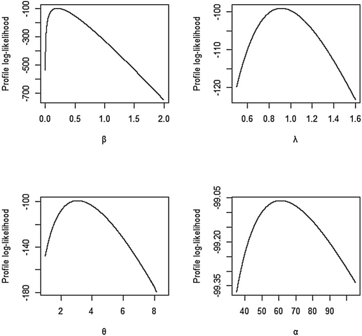
The profile likelihood plots of the EAPLL parameters for failure times data.

Figure 15.

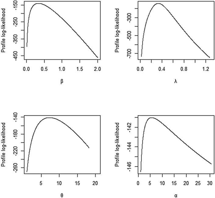
The profile likelihood plots of the EAPLL parameters for carbon fibers data.

Figure 16.

The profile likelihood plots of the EAPLL parameters for time to failure data.

Conclusions

In this paper, we introduce a flexible distribution called the exponentiated alpha-power log-logistic (EAPLL) distribution. Its failure rate can be increasing, reversed-J shaped, decreasing, increasing-decreasing-increasing, bathtub, decreasing-increasing-decreasing, or inverted bathtub, providing considerable flexibility in modeling diverse types of data. Some of the mathematical properties of the EAPLL model are explored. Furthermore, the EAPLL parameters are estimated using eight different estimation methods. Simulation studies evaluate the performance of these estimators, revealing that all classical estimators perform well, with the maximum product of spacing (MPS) method showing superior performance. Therefore, the MPS method is recommended for estimating EAPLL parameters.

The usefulness of the EAPLL distribution is demonstrated using three real-life survival data sets. It provides a better fit as compared to some competing log-logistic distributions. To illustrate the uniqueness and reliability of the parameter estimates, profile likelihood plots are provided. While the EAPLL distribution offers significant advantages such as flexibility in failure rate modeling and better data fit, it may also have some drawbacks, including potential complexity in parameter estimation and the necessity for robust computational tools.

Additionally, the selection of real data sets for the demonstration was based on their varied characteristics, ensuring a comprehensive evaluation of the EAPLL model’s applicability. This thorough approach highlights both the practical relevance and potential limitations of the distribution in real-world scenarios.

Future work could explore the application of the EAPLL distribution in other fields beyond survival analysis, developing more efficient computational methods for parameter estimation, and investigating its performance in large-scale data environments. By addressing these avenues, we aim to enhance further the utility and robustness of the EAPLL model in statistical modeling and analysis.

The proposed EAPLL model is expected to offer valuable insights in survival analysis and other related fields, providing a flexible and powerful tool for understanding complex data structures and uncertainty in various phenomena.

Author contributions

V.K. and A.Z.A wrote the main manuscript text, and all authors reviewed the manuscript. A.W., O.N., and A.Z.A. supervised the writing of the manuscript. All authors, V.K., A.W., O.N., H.M.A., A.S.A., and A.Z.A., worked on the software, and V.K., and A.Z.A. prepared all the figures. All authors, V.K., A.W., O.N., H.M.A., A.S.A., and A.Z.A., reviewed the concept of the manuscript.

Data availability

All data generated or analyzed during this study are included in this published article.

Competing interests

The authors declare no competing interests.

References

- 1.Muse, A. H. et al. Bayesian and frequentist approaches for a tractable parametric general class of hazard-based regression models: An application to oncology data. Mathematics10, 3813 (2022). 10.3390/math10203813 [DOI] [Google Scholar]
- 2.Mastor, A. B., Ngesa, O., Mungatu, J., & Afify, A. Z. The extended exponential-Weibull accelerated failure time model with applications to cancer data set. In Engineering (ICMASE 4–7 July 2022) Technical University of Civil Engineering Bucharest. Vol. 69 (2022).
- 3.Lawless, J. F. Statistical Models and Methods for Lifetime Data (Wiley, NY, 2011). [Google Scholar]
- 4.Khan, S. A. Exponentiated Weibull regression for time-to-event data. Lifetime Data Anal.24, 328–354 (2018). 10.1007/s10985-017-9394-3 [DOI] [PubMed] [Google Scholar]
- 5.Azzalini, A. & Valle, A. D. The multivariate skew-normal distribution. Biometrika83, 715–726 (1996). 10.1093/biomet/83.4.715 [DOI] [Google Scholar]
- 6.Eugene, N., Lee, C. & Famoye, F. Beta-normal distribution and its applications. Commun. Stat.-Theory Methods31, 497–512 (2002).
- 7.Zografos, K. & Balakrishnan, N. On families of beta-and generalized gamma-generated distributions and associated inference. Stat. Methodol.6, 344–362 (2009). 10.1016/j.stamet.2008.12.003 [DOI] [Google Scholar]
- 8.Cordeiro, G. M. & de Castro, M. A new family of generalized distributions. J. Stat. Comput. Simul.81, 883–898 (2011). 10.1080/00949650903530745 [DOI] [Google Scholar]
- 9.Mudholkar, G. S. & Srivastava, D. K. Exponentiated Weibull family for analyzing bathtub failure-rate data. IEEE Trans. Reliab.42, 299–302 (1993). 10.1109/24.229504 [DOI] [Google Scholar]
- 10.Alzaatreh, A., Lee, C. & Famoye, F. A new method for generating families of continuous distributions. Metron71, 63–79 (2013). 10.1007/s40300-013-0007-y [DOI] [Google Scholar]
- 11.Cordeiro, G. M., Afify, A. Z., Yousof, H. M., Pescim, R. R. & Aryal, G. R. The exponentiated Weibull-H family of distributions: Theory and applications. Mediterr. J. Math.14, 1–22 (2017). 10.1007/s00009-017-0955-1 [DOI] [Google Scholar]
- 12.Mahdavi, A. & Kundu, D. A new method for generating distributions with an application to exponential distribution. Commun. Stat.-Theory Methods46, 6543–6557 (2017).
- 13.Malik, A. S. & Ahmad, S. P. An extension of log-logistic distribution for analyzing survival data. Pak. J. Stat. Oper. Res.16, 789–801 (2020). 10.18187/pjsor.v16i4.2961 [DOI] [Google Scholar]
- 14.Bennett, S. Log-logistic regression models for survival data. J. R. Stat. Soc. Ser. C Appl. Stat.32, 165–171 (1983).
- 15.De Santana, T. V. F., Ortega, E. M. M., Cordeiro, G. M. & Silva, G. O. The Kumaraswamy-log-logistic distribution. J. Stat. Theory Appl.11, 265–291 (2012). [Google Scholar]
- 16.Gui, W. Marshall-Olkin extended log-logistic distribution and its application in minification processes. Appl. Math. Sci.7, 3947–3961 (2013). [Google Scholar]
- 17.Tahir, M. H., Mansoor, M., Zubair, M. & Hamedani, G. McDonald log-logistic distribution with an application to breast cancer data. J. Stat. Theory Appl.13, 65–82 (2014). 10.2991/jsta.2014.13.1.6 [DOI] [Google Scholar]
- 18.Lemonte, A. J. The beta log-logistic distribution. Braz. J. Probab. Stat.28, 313–332 (2014). 10.1214/12-BJPS209 [DOI] [Google Scholar]
- 19.Shakhatreh, M. K. A new three-parameter extension of the log-logistic distribution with applications to survival data. Commun. Stat. Theory Methods47, 5205–5226 (2018). 10.1080/03610926.2017.1388399 [DOI] [Google Scholar]
- 20.Lima, S. R. & Cordeiro, G. M. The extended log-logistic distribution: Properties and application. An. Acad. Bras. Ciênc.89, 03–17 (2017). 10.1590/0001-3765201720150579 [DOI] [PubMed] [Google Scholar]
- 21.Aldahlan, M. A. Alpha power transformed log-logistic distribution with application to breaking stress data. Adv. Math. Phys.1–9, 2020 (2020). [Google Scholar]
- 22.Chaudhary, A. K. Frequentist parameter estimation of two-parameter exponentiated log-logistic distribution. NCC J.4, 1–8 (2019). 10.3126/nccj.v4i1.24727 [DOI] [Google Scholar]
- 23.Chaudhary, A. K. & Kumar, V. Bayesian estimation of three-parameter exponentiated log-logistic distribution. Int. J. Stat. Math.9, 66–81 (2014). [Google Scholar]
- 24.Nassar, M., Kumar, D., Dey, S., Cordeiro, G. M. & Afify, A. Z. The Marshall-Olkin alpha power family of distributions with applications. J. Comput. Appl. Math.351, 41–53 (2019). 10.1016/j.cam.2018.10.052 [DOI] [Google Scholar]
- 25.Ramos, M. W. A., Cordeiro, G. M., Marinho, P. R. D., Dias, C. R. B. & Hamedani, G. G. The Zografos-Balakrishnan log-logistic distribution: Properties and applications. J. Stat. Theory Appl.12, 225–244 (2013). 10.2991/jsta.2013.12.3.2 [DOI] [Google Scholar]
- 26.Adeyinka, F. S. & Olapade, A. K. On transmuted four parameters generalized log-logistic distribution. Int. J. Stat. Distrib. Appl.5, 32–37 (2019). [Google Scholar]
- 27.Alzaghal, A. & Aldenı, M. A versatile family of generalized log-logistic distributions: Bimodality, regression, and applications. Hacettepe J. Math. Stat.51, 857–881 (2022). [Google Scholar]
-
28.Job, O. & Ogunsanya, A. S. Weibull log logistic
exponential
distribution: Some properties and application to survival data. Int. J. Stat. Distrib. Appl.8, 1–13 (2022). [Google Scholar]
- 29.Mead, M. E., Afify, A. Z. & Butt, N. S. The modified Kumaraswamy Weibull distribution: Properties and applications in reliability and engineering sciences. Pak. J. Stat. Oper. Res.16, 433–446 (2020). 10.18187/pjsor.v16i3.3306 [DOI] [Google Scholar]
- 30.Kariuki, V., Wanjoya, A., Ngesa, O. & Alqawba, M. A flexible family of distributions based on the alpha power family of distributions and its application to survival data. Pak. J. Stat.39, 237–258 (2023). [Google Scholar]
- 31.Moors, J. J. A. A quantile alternative for kurtosis. J. R. Stat. Soc. Ser. D (The Statistician)37, 25–32 (1988). [Google Scholar]
- 32.Al-Aqtash, R., Lee, C. & Famoye, F. Gumbel-Weibull distribution: Properties and applications. J. Mod. Appl. Stat. Methods13, 11 (2014). 10.22237/jmasm/1414815000 [DOI] [Google Scholar]
- 33.Abouelmagd, T. H. M. et al. Extended Weibull log-logistic distribution. J. Nonlinear Sci. Appl.12, 523–534 (2019). 10.22436/jnsa.012.08.03 [DOI] [Google Scholar]
- 34.Nasiru, S., Mwita, P. N. & Ngesa, O. Exponentiated generalized exponential Dagum distribution. J. King Saud Univ.-Sci.31, 362–371 (2019).
- 35.Hemeda, S. Additive Weibull log logistic distribution: Properties & application. J. Adv. Res. Appl. Math. Stat.3, 8–15 (2018). [Google Scholar]
- 36.Afify, A. Z., Hussein, E. A., Alnssyan, B. & Mahran, H. A. The extended log-logistic distribution: properties, inference, and applications in medicine and geology. J. Stat. Appl. Probab.12, 1155–1580 (2023). [Google Scholar]
- 37.Alfaer, N. M., Gemeay, A. M., Aljohani, H. M. & Afify, A. Z. The extended log-logistic distribution: inference and actuarial applications. Mathematics9, 1386 (2021). 10.3390/math9121386 [DOI] [Google Scholar]
- 38.Muse, A. H., Mwalili, S. M. & Ngesa, O. On the log-logistic distribution and its generalizations: A survey. Int. J. Stat. Probab.10, 93 (2021). 10.5539/ijsp.v10n3p93 [DOI] [Google Scholar]
Associated Data
This section collects any data citations, data availability statements, or supplementary materials included in this article.
Data Availability Statement