

Abstract
We report high resolution measurements of the stable water isotope ratios (δ18O, δD) from the Mount Brown South ice core (MBS, 69.11° S 86.31° E). The record covers the period 873 - 2009 CE with sub-annual temporal resolution. Preliminary analyses of surface cores have shown the Mount Brown South site has relatively high annual snowfall accumulation (0.3 metres ice equivalent) with a seasonal bias toward lower snowfall during austral summer. Precipitation at the site is frequently related to intense, short term synoptic scale events from the mid-latitudes of the southern Indian Ocean. Higher snowfall regimes are associated with easterly winds, while lower snowfall regimes are associated with south-easterly winds. Isotope ratios are measured with Infra-Red Cavity Ring Down Spectroscopy, calibrated on the VSMOW/SLAP scale and reported on the MBS2023 time scale interpolated accordingly. We provide estimates for measurement precision and internal accuracy for δ18O and δD.
Subject terms: Palaeoclimate, Infrared spectroscopy, Cryospheric science
Background & Summary
With a plethora of paleoclimatic information contained in their continuous stratigraphy, Antarctic ice cores constitute unique archives of past climate variability. Deep cores drilled in the low accumulation areas of East Antarctica provide a picture of the climate spanning up to 800,000 y1,2, whereas higher accumulation areas can typically yield paleoclimatic signals of high temporal resolution (decadal to subannual)3–5. The isotopic composition of polar ice is a valuable paleoclimatic proxy of past hydrological cycle conditions and atmospheric temperatures6–9. It is commonly expressed with the δ notation10 as the deviation of a sample’s isotopic ratio relative to that of a reference water expressed in per mille (‰) as: δi = (iRsample/iRV SMOW − 1) × 1000 where 2R = 2H/1H and 18R = 18O/16O. The internationally established reference scale is defined by two waters, the Vienna Mean Ocean Water (VSMOW) and the Standard Light Antarctic Precipitation (SLAP), both materials, stored, maintained and distributed by the International Atomic Energy Agency11.
In this work we present dual measurements (δ18O, δD) from a new high-resolution ice core from East Antarctica, the Mount Brown South (MBS) ice core (69.11° S 86.31° E, 2084 m elevation). The MBS ice core was drilled during the 2017/2018 austral summer field season addressing a substantial need for millennial-length, high-resolution climate records from the Indian Ocean sector of East Antarctica12. The isotopic record presented here is a compilation of discrete analyses (4–104 m depth; 0.03 m resolution) and continuous flow analysis (CFA) (94 – 295 m depth; 0.005 m resolution). The record is 295 m long and represents 1135 years (873–2009 CE)13. We used state of the art Cavity Ring Down Spectroscopy (CRDS) assuring exceptional data quality with respect to both precision and accuracy together with quality metrics to quantify measurement noise as a function of depth. In particular, for the CFA part of the record we used innovative in-house developed methods with respect to ice core sample handling and flash, fractionation-free vaporisation14 that resulted in ultra-high resolution sub-annual isotope signals.
The MBS water isotope record will be useful for a wide range of studies aiming to understand the climate variability of the Southern Hemisphere spanning centennial to inter-annual time scales. Covering a time frame before, as well as during the observational window, it can be used for forcing climate models at high resolution. In particular, the location of the MBS drilling site could potentially allow for studies focusing on the dominant climate modes of the South Hemisphere, the El Niño Southern Oscillation (ENSO) and the Southern Annular Mode (SAM), as well as interdecadal variability stemming from the Pacific Ocean12,13,15.
A small part of the record (4-20 m of the δ18O signal) has previously been presented in the study of Jackson et al.16, which focuses on the recent climatology of the site and its implications for the interpretation of the δ18O signal in the core. An investigation of ENSO signals aparent in the MBS record has been performed in15 also using the top 20 m of the high resolution water isotope record.
Methods
The Mount Brown South (MBS) Ice Core
The ice core site
The MBS ice core site is located near the boundary of Princess Elisabeth and Wilhelm II Land in East Antarctica, 380 km inland and to the west of Australia’s Davis Station. It is located in the Indian Ocean sector of coastal East Antarctica, a region poorly represented by high-resolution ice core records, limited to several short cores (up to 350 years) in Princess Elizabeth Land17 and the Law Dome ice core18 (Fig. 1). The Law Dome record spans up to 90,000 years and is available at annual or sub-annual resolution for the past 2000 years. It has been widely used to reconstruct regional climate variability of coastal East Antarctica19 as well as hydroclimate variability in both southwest Western Australia5,20,21 and eastern Australia22,23 due to synoptic-scale weather and climate links between coastal East Antarctica and Australia24.
Fig. 1.
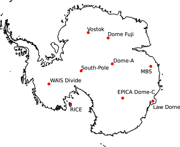
Map of Antarctica and location of prominent ice core drilling sites.
The MBS ice core site was selected following an extensive site-selection study12 to fill a critical gap in the current network of ice core records. Seven criteria were considered when selecting the ice core site including (i) at least 1000-year-old ice at depths of 300 m; (ii) summer surface temperatures <0°C to minimise melt; (iii) high-resolution (sub-annual) requiring accumulation of >250 mm a−1 (iv) minimal surface reworking; (v) located on a ridgeline or dome; (vi) teleconnection with mid-latitude climate; (vii) complementary to existing records. The final site, Mount Brown South, meets all of these requirements and expands the current network of high-resolution temperature and hydroclimate proxies. An annually resolved chronology for the MBS ice core, MBS2023, was developed in Vance et al.13 using annual layer counting and alignment to known volcanic horizons.
Drilling and sampling
During the 2017/18 austral summer field season, a 295 m long ice core with a diameter of 98 mm was drilled from 4 m below the surface using a Hans Tausen drill25. Wet drilling started at a depth of 93 m (driller’s depth) using Estisol 140 as drilling liquid. The core was cut in 1 m sections (ice core bags) in the field and transported to the ice core facilities of the Institute for Marine and Antarctic studies (IMAS) in Hobart, Australia for further processing. Visual features in the ice such as breaks, wind crusts and bubble free layers were thoroughly logged prior to further sectioning. Following the cutting scheme shown in Fig. 2, samples were prepared at a temperature of −18°C using a trace-clean band saw. Two rectangular rods measuring 34 × 34 mm were cut for the purpose of CFA and for trace ion chemistry analysis. The two wedges on each side of the square rods were collected for tephra and discrete water stable isotope analysis. The latter was sampled at a resolution of 30 mm.
Fig. 2.
Cross section of the MBS ice core showing the cutting scheme of the ice core samples.
The CFA square rods were subsequently transported to Copenhagen, Denmark for further sample preparation and subsequent chemical and water isotope analysis. Typically, 1-2 mm from the ends of the CFA rods were carefully shaved off in order to minimise contamination of the chemical impurity analysis. For rods with slightly slanted ends the removal of material was adjusted and documented accordingly. For the same reason, we removed internal breaks and then shaved off and flattened the ice on each side of the break. The lengths of all the ice pieces were carefully documented, prior as well as after the processing of breaks and edges of the CFA rods.
Stable Isotope Analysis – Cavity Ring Down Spectroscopy
Two versions of the Picarro water isotope analyzer (Picarro L-2130i and L-2140i) were used for the analysis of the discrete and continuous samples. The Picarro L-21xxi water isotopes analyzers are Cavity Ring Down Spectrometers (CRDS), operating in the near-IR region at 7200 cm−1 and both operate on the same spectroscopic principles. The analyzer uses a continuous emission diode laser source coupled to a high-finesse, 3-mirror, V-shaped cavity. Analysis takes place in the gas phase at a cavity pressure of 67 mbar (50 Torr) and a temperature of 80°C. Precise control of the cavity’s pressure and temperature (≈2mbar, 1mK, 1-σ) is key for optimal instrument performance. This is achieved by the instrument’s control software continuously adjusting the position of two proportional valves up- and downstream of the optical cavity maintaining stable pressure and by driving heat elements installed in a well insulated and ventilated box that contains the optical cavity. Temperature and pressure stability is also facilitated by maintaining a stable laboratory temperature and a stable gas flow at the inlet of the instrument. The sample flow through the optical cavity is .
Discrete samples water isotope analysis; 0-104 m depth
The upper 100 m of the ice core were analysed at the Australian Antarctic Division (AAD) Ice Core laboratory facilities at IMAS, Hobart (4.0–74.2 m) and the Australian National University (ANU), Canberra (74.2–100.0 m), for interlaboratory comparison purposes using a discrete sampling scheme. The discrete ice core samples were stored frozen at IMAS, Hobart after processing. For the section analysed at the ANU, Canberra, samples were transported frozen and remained frozen until analysis. The ice samples were melted at room temperature, whereafter 200 μL were transferred into 2 mL screw thread glass vials (Fisherbrand 033918) fitted with 300 μl polyspring inserts (Thermo Scientific C4010-S630) and sealed with silicone/PTFE septum caps (Thermo Scientific THC09-15-1178). The ice samples at IMAS were defrosted in a fridge at 4°C overnight. Aliquots of 250 μL were transferred into 2 mL snap top glass vials (Agilent 5182-0546) fitted with 250 μL pulled point glass vial inserts (Agilent 5183-2085) and sealed with PTFE/red silicone snap caps (Agilent 5182-0564).
Instrumentation used for discrete samples
Stable water isotope analysis on the discrete samples was performed using two variants of the Picarro L21xx-i analyzer with similar performance characteristics with respect to precision and sample handling. At IMAS, Hobart, a Picarro L2130-i stable water isotope analyzer was used, while the L2140-i variant was used at ANU, Canberra. At both IMAS, Hobart, and ANU, Canberra, the Picarro analyzers were coupled to the Picarro A0211 vaporizer and the Picarro A0325 autosampler. Pressurized dry air () was used as carrier gas and mixed with the injected sample in the vaporizer’s sample cell at a temperature of 110°C, regulated by means of PID control. The water sample was injected using a 10 μL syringe ( SGE 10R-BT-GT-0.47C) with an injection volume of 1.8 μL liquid water at IMAS, Hobart and 1.5 μL at the ANU, Canberra. After an equilibration time of 60 s in the vaporizer’s cell, the vapor-air mixture was gradually introduced into the optical cavity for spectroscopic analysis. The instruments comprising each experimental setup as well as the specifications of the autosampler injection methods are given in Tables 1 and 2 respectively.
Table 1.
Instrument specifications for analyses at IMAS, Hobart and ANU, Canberra.
| Component | IMAS, Hobart | ANU, Canberra |
|---|---|---|
| Picarro Model | Picarro L2130-i | Picarro L2140-i |
| Autosampler | Picarro A0325 | Picarro A0325 |
| Vaporizer | Picarro A0211 | Picarro A0211 |
| Syringe | Trajan SGE 002250 10 μL | Trajan SGE 002250 10 μL |
Table 2.
Autosampler injection method for the Picarro L2130-i (analyses performed at IMAS, Hobart) and the Picarro L2140-i (analyses performed at ANU, Canberra).
| Property | Picarro L2130-i | Picarro L2140-i |
|---|---|---|
| Syringe Volume | 10 μL | 10 μL |
| Sample Volume | 1.8 μL | 1.5 μL |
| Fill Speed | 2.5 μL/s | 500 nL/s |
| Fill Strokes | 1 | 1 |
| Inject Speed | 2.0 μL/s | 500 nL/s |
| Pre Injection Delay | 0 s | 7 0 s |
| Post Injection Delay | 1.0 s | 1.0 s |
Run configuration for discrete analyses
Analysis of discrete samples in Hobart and Canberra followed similar protocols with small deviations. At both facilities, an analytical sequence consisted of calibration sequences bracketing “unknowns", with isotopic values expressed as per mil (‰) and relative to the Vienna Standard Mean Oceanic Water (VSMOW). A typical analytical sequence using the AAD Picarro L2130-i consisted of 30 “unknowns", while a sequence at the ANU, Canberra consisted of 20 “unknowns".
In Hobart, three in-house calibration standards were used (tap water, Dome Summit South (DSS) and Lambert Glacial Basin (LGB)), as well as a laboratory reference water sample or check standard, MBS, treated as an unknown (Table 3). The check standard (MBS) was analysed after 10 unknown samples to monitor run stability. Analysis was performed in “High-Precision" mode with methods that enabled analysis of a single injection in ~8 mins. A typical analytical run with calibration standards and 30 “unknowns" was completed in just over 24 hours. The analysis of each standard (including the check standard) consisted of 8 injections, with the first 4 injections discarded in order to account for memory effects. The “unknowns” were analysed sequentially with increasing depth to reduce the memory effects. Each “unknown” measurement consisted of 4 injections with the first injection discarded.
Table 3.
ANU local standards used for the discrete analyses.
| Standard | δ18O (‰) | δD (‰) |
|---|---|---|
| VSMOW | 0 | 0 |
| SLAP | − 55.5 | − 427.5 |
| DSS | − 22.8 | − 178.1 |
| MBS | − 32.4 | − 258.1 |
| LGB | − 39.0 | − 309.6 |
All values are given in ‰ with respect to VSMOW.
In Canberra, we used two in-house calibration standards (DSS and LGB), as well as a check standard, MBS, treated as an unknown. The check standard (MBS) was analysed between unknown samples #10 and #11 to monitor run stability, as well as at the mid-point of each calibration sequence. The analysis of each standard (including the check standard) consisted of 20 injections, with the first 13 injections discarded in order to account for memory effects. The “unknowns” were analysed sequentially with increasing depth to reduce the memory effects associated with large isotopic steps. Each “unknown” measurement consisted of 10 injections with the first four discarded. Analysis at the ANU, Canberra was performed in the Picarro “High-Precision” mode, which utilises injection times of ~9 min (total time ~1.5 hours per sample). A run consisted of several analytical sequences and thus lasted several days.
Continuous Flow Analysis (CFA)
The more recent development of high-resolution Continuous Flow Analysis (CFA) techniques based on the continuous melting of ice core samples26–29 has yielded unprecedented records of chemical impurities30–33. We continuously melt an ice core rod over a custom designed and manufactured heated melt plate29 and further debubble and distribute the liquid sample stream to an array of analyzers. This approach has the potential to yield multi-component, very high resolution data sets on a common depth scale with a massively improved throughput compared to the laborious relatively low-resolution analysis performed in the traditional way using ion chromatography or inductively coupled plasma mass spectrometry.
Laser spectroscopy techniques employing Cavity Enhanced/Cavity Ring Down Spectroscopy (CRDS) configurations have made it possible to measure trace gas concentrations and stable water isotope ratios in a continuous flow mode with minimal sample preparation34–36. Interfacing these techniques to existing CFA systems allowed for continuous, high-resolution records of CH437,38 as well as water stable isotope records (δ18O, δD)39–42 in ice cores with significant improvements in precision, accuracy, sample consumption and throughput.
The Copenhagen CFA system
The Copenhagen CFA system is optimized for high depth resolution capable of analysing an array of chemical parameters such as conductivity, insoluble dust, Ca2+, , Na+ and pH29,32,43. Following a modular approach, more components can be incorporated in the synchronous analysis. The system utilizes an aluminum melter with an outer sample square ring measuring 34 × 34 mm and an inner sample square ring measuring of 26 × 26 mm (Fig. 2 in29). The melt rate is controlled by the melter’s temperature maintained by four 125 W Mickenhagen heat cartridges in combination with a J-type thermocouple and a PID–loop control unit (dTRON 308, Jumo). A draw wire sensor incorporating an optical encoder (WayCon SX-80) records the melt speed with a sensitivity γ = 25 counts mm−1.
During the campaign the nominal melting speed of yielded a clean, central line sample flow of maintained by a peristaltic pump (Ismatec IPC-16). This sample contained ≈10% air due to the air bubbles occluded in the ice core. Removal of the air occurred in a homemade Polyether-Ether-Ketone (PEEK) flat triangular-cell debubbler following a simple buoyancy principle (Fig. 3 in29). Downstream of the debubbler, the air-free flow equalled of which was pumped further for water isotope analysis. The liquid water-air mixture with a flow of was forwarded to a gas extraction membrane (3M, Liqui-Cel MM-0.75 × 1 Series) for further gas-liquid separation and subsequent CH4 analysis. A more thorough presentation of the chemical analysis of the MBS core accompanied by the adjoined data records will follow in a separate publication. The dataset can be accessed at the Australian Antarctic Data Center44.
Continuous flash vaporisation for water isotope analysis
In Fig. 3 we present the water isotope analysis segment of the CFA system. We follow a slightly modified version of the CFA-water isotope system presented in14,39 in which a microflow of liquid water is continuously injected and flash-vaporised in a PID-regulated 170°C oven (T2 in Fig. 3) to which we introduce a stream of dry air (<30 ppmV) with a flow of . The liquid microflow is in the order of 2 and is achieved by sampling a higher flow of 0.4 with a fused silica capillary (ID 50 μm) in a tee-split (T1 in Fig. 3) configuration. The high flow of 0.4 is maintained by the peristaltic pump P1 (Ismatec ISM597D) that pulls the sample through V1, a 6-port selection valve (Vici C25-3186EMH). The latter is used to choose between the CFA sample line or glass containers with water isotope standards or a glass container with background deionised water. We used amber glass 250 ml bottles (Duran GL45, 250 ml, S/N: 818063604) with GL-45 thread safety caps (JR-S-11011) and inlet solvent stainless steel filters (IDEX A-302) with a porosity of 10 μm. Upstream of V1, a parallel configuration of two inline filters (IDEX A-313) fitted with stainless steel 20 μm porosity frits (IDEX A-120) ensures that the CFA sample stream is free of particles that can deteriorate the smooth operation of the selection valve or the oven capillary. Downstream of the vaporisation oven T2, the vapour sample is introduced into an open split (T3 in Fig. 3) consisting of a stainless steel 1/16 inch tee-split (Swagelok SS-100-3), through which the analyzer pulls the necessary flow of .
Fig. 3.

Block diagram of the water isotope analysis part of the CFA system. For a complete description of the system’s components, the reader is referred to Section Methods.
Our flash-evaporation approach has been shown to yield a vapor sample flow that is not affected by isotopic fractionation issues, thus allowing for a very stable performance with the possibility to also average over longer times in order to achieve very high signal-to-noise ratios. The practically zero-dead volume flow system minimises sample dispersion such that ultra high resolution measurements are possible39,45. For optimal results we operate the spectrometer in the [H2O] range of 10,000-23,000 ppmV. Tuning of the [H2O] level can be achieved with a needle valve installed on the dry air line, which in combination with the open split T3, disturbs neither the sample flow nor the pressure in the optical cavity.
The MBS CFA campaign
The analysis of the MBS core took place in Copenhagen, at the CFA lab of the Ice and Climate group at the Niels Bohr Institute over 13 working days during October 2019. A total of 195.386 m of ice was processed through the CFA system equivalent to 201.634 m of ice core length when including the pieces of ice removed during the processing of the breaks. Depthwise, the record spans the range 93.082-294.712 m corresponding to the age interval 1736-873 CE13. In Fig. 4 we show the processing throughput during the campaign.
Fig. 4.
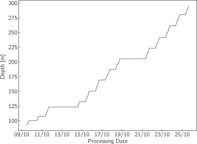
Analysis production during the MBS CFA campaign spanning 13 working days (09/10/2019 - 25/10/2019).
CFA isotope processing sequence
From the water isotope point of view, a typical CFA processing day consists of the Idle, Calibration and Run modes (Fig. 5). In the Idle, mode the selection valve V1 connects to the DI water container feeding the system overnight. These sections were used in order to evaluate the performance of the system with respect to stability, accuracy and long term averaging, by means of Allan variance tests14,46 (section Technical Validation).
Fig. 5.

Example of the sequence of events during an analysis day of the MBS CFA campaign. We plot the raw δD signal (left axis) and the water concentration levels in the laser spectrometers optical cavity during a period of 24 hours on the 22nd of October. The pale red, blue and yellow areas of the plot mark the IDLE, VSMOW-SLAP calibration and ice core run phases of the day. The pale green areas correspond to the time when the isotope system was on IDLE mode while the chemical analysis part of the CFA system was being calibrated.
The processing day starts with a VSMOW-SLAP calibration (section “Cal” colored light blue in Fig. 5) a procedure that involves three local water isotope standards, with the middle one being used as a “check” standard for estimation of the systems accuracy. Each standard water is run for 20 min resulting in a calibration procedure that lasts 60 min in total. The whole sequence can be initiated and monitored remotely via a homemade Python-based valve control and data acquisition script.
When on “Run” mode the system is measuring ice core sample and the selection valve V1 is connected to the “CFA” sample port. As seen in Fig. 5, a processing day contains two sample runs each consisting of 9 ice core bags equivalent to ≈9 m of ice. In the particular example of Fig. 5 from the 22nd of October, the first run (Run #224) consists of the ice core bags 224-232 and the second run (Run #233) consists of ice core bags 233-241. A necessary calibration procedure for the chemical analysis results in a period of Idle mode between the two runs that can last 1-2 h (green areas in Fig. 5).
Data analysis - Discrete sampling
VSMOW-SLAP calibration - Discrete analysis
Three local standards calibrated against the IAEA reference waters SLAP and VSMOW were used to calibrate the raw δ18O and δD signals to the VSMOW-SLAP scale. All of the in-house standards consist of bulk Antarctic meltwater samples collected from three locations in Antarctica: Dome Summit South (DSS), Lambert Glacial Basin (LGB) and Mount Brown South (MBS). (Table 3). We follow the IAEA recommended procedure11 and use the most enriched (DSS) and depleted (LGB) local standards to build a two-point fixed calibration line as:
| 1 |
where δ’ represents the calibrated signal and the slope α and the intercept β are given by:
| 2 |
| 3 |
The additional “MBS" standard was analysed several times during each run sequence in order to assess the internal accuracy and precision of each analytical run after calibration to the VSMOW-SLAP scale as described above.
Data analysis - CFA
VSMOW-SLAP calibration - CFA analysis
Reporting of the δ18O and δD signals on the VSMOW-SLAP scale requires a calibration step similar to the one taken for the discrete data and described in section. Following an approach similar to14,39 we used three local water isotopic standards calibrated against the primary IAEA reference waters VSMOW and SLAP (Table 4) in order to (i) produce a two fixed-point calibration line defined by the two extreme local standards “–40” and “–22” and (ii) estimate the system’s accuracy by comparing the value of the middle “NEEM” standard post calibration with its nominal value (Table 4). Using the prime notation for the calibrated δ signals, raw δ measurements are calibrated on the VSMOW-SLAP scale according to the calibration line in Eq. (4)
| 4 |
where the slope α and the intercept β are given by:
| 5 |
| 6 |
From Eqs. (4)–(6) we calculate the VSMOW calibrated value of the middle “check”standard, which is then compared to the nominal VSMOW value of the “check” standard water (Table 4).
Table 4.
Copenhagen local standards used for the MBS record VSMOW-SLAP calibrations.
| Name | δ18O | δD |
|---|---|---|
| − 22 | − 21.86 | − 168.32 |
| NEEM | − 33.52 | − 257.2 |
| − 40 | − 40.02 | − 311.1 |
All values are given in ‰ with respect to VSMOW.
Depth assignment
Assigning the depth on each CFA run requires the alignment of the wire depth encoder signal with the δ18O and δD signals. The WayCon SX-80 wire encoder delivers a digital signal with a resolution γ = 25 countsmm−1. The melted length as a function of time can then be calculated by the integration of the differential counts signal as
| 7 |
where ti and tf denote the start and end of the CFA run. Following the detailed logging of the CFA sample rods with respect to internal breaks’ positions and lengths as well as the top depths of every ice core bag it is possible to reconstruct the depth vector z(t) of each CFA run as a function of elapsed measurement- and Unix Epoch time. In order to transfer the depth scale on the water isotope data, we first locate the beginning and the end of each CFA run in the δD signal. Due to the isotopically heavier value of the background DI water relative to the isotopically light Antarctic sample, CFA run segments are easily distinguishable. We search for the minimum and maximum values of a smoothed version (10-point Bartlett window) of the derivative of the δD signal corresponding to the beginning and end of CFA run respectively. Finally, linear interpolation of the z(t) signal on the time vector of the isotope signal sets the isotope measurements on the depth scale of the ice core. In Fig. 6 we show an example of locating the beginning and end of CFA run 224 based on the δD signal and its derivative. We also show the result of the melted length l(t) calculation based on Eq. (7) without (solid line) and with (dashed-dotted line) the core breaks taken into consideration.
Fig. 6.

δD of Run 224. The run contains the ice core bags 224-232 and spans ≈9 m. The smoothed derivative of the δD signal (blue curve) is used for the identification of the beginning and the end of the run. With solid black, we plot the run length signal as measured with the wire optical encoder and with the dashed line we show the length signal corrected for the logged internal breaks.
Data analysis: The age scale
An age scale has been developed for the MBS ice core record, hereafter referred to as MBS2023, resulting in a chronology spanning 1137 a (873–2009 CE)47. The construction of the chronology utilises a layer-counting approach, in combination with aligning volcanic horizons by comparing the non-sea sulfate signal () in the MBS, Law Dome48, Roosevelt Island Ice Core49 as well as the West Antarctic Ice Sheet (WAIS) Divide chronology, WD201431. Annual layers are identified and counted visually in the sea salt and non-sea sulfate signals, the former yielding maxima in austral winter and the latter in austral summer. This type of variability results additionaly in signal peaks for the sulfate to chloride ratio during the austral summer50. Austral summer water isotope maxima (δ18O and δD) are also used in the counting of the annuals. For a detailed description of the dating methods the reader is referred to the dedicated paper by Vance et al.13.
Data Records
The dataset can be found in the Australian Antarctic Data Center (AADC) repository51. It consists of two sub-datasets in files mbs_water_isotopes_a.txt and mbs_water_isotopes_b.txt. The _a.txt file contains the discrete data on the 0.03 m resolution spanning the depth range 4-104 m. The temporal resolution of this record varies from ≈ 17 points a−1 at the top of the record, to ≈9 points a−1 at the bottom of the record. The CFA data can be found in the _b.txt file covering a depth range between 93 and 294.7 m. With a depth resolution of 0.005 m this dataset has a temporal resolution of ≈57 points a−1 at the top of the record (93 m),while at the bottom of the record (294.7 m) the resolution is ≈45 points a−1. We also provide the full record on the MBS2023 timescale only and an annual time resolution. The full record can be found in mbs_water_isotopes_annual.txt. In this merged record we use the discrete data from year 2008 CE until year 1695 CE. Thereafter and until the year 873 CE the record is based on the CFA measurements. In Tables 5, 6 and 7 we list and describe the variables included in the data record for the discrete samples and the CFA analysis respectively. The δ18O signal of the full record is presented on the MBS2023 age scale in Fig. 7
Table 5.
Name and description of the variables included in the data file mbs_water_isotopes_a containing the discrete samples dataset.
| Variable | Unit | Description |
|---|---|---|
| Depth_Top | m | Top Depth of data sample |
| Depth_Mid | m | Middle Depth of data sample |
| Depth_Bottom | m | Bottom Depth of data sample |
| MBS2023 | a CE | Date based on the MBS2023 age scale for the middle depth of the sample |
| d18 | ‰ | δ18O of the sample |
| dD | ‰ | δD of the sample |
| d18_precision | ‰ | 1-σ of noise for δ18O estimated from the ”MBS” standard treated as unknown |
| dD_precision | ‰ | 1-σ of noise for δDestimated from the ”MBS” standard treated as unknown |
| d18_accuracy | ‰ | Internal accuracy for δ18O estimated from the ”MBS” standard treated as unknown |
| dD_accuracy | ‰ | Internal accuracy for δD estimated from the ”MBS” standard treated as unknown |
Table 6.
Name and description of the variables included in the data file mbs_water_isotopes_b containing the CFA dataset.
| Variable | Unit | Description |
|---|---|---|
| Depth | m | Depth of data point |
| MBS2023 | a CE | Date based on the MBS2023 age scale |
| d18 | ‰ | δ18O of the sample |
| dD | ‰ | δD of the sample |
| sigma_d18 | ‰ | 1-σ of measurement noise for δ18O calculated from the PSD |
| sigma_dD | ‰ | 1-σ of measurement noise for δD calculated from the PSD |
Table 7.
Name and description of the variables included in the data file mbs_water_isotopes_annual containing the merge of the discrete and the CFA datasets on annual resolution.
| Variable | Unit | Description |
|---|---|---|
| MBS2023 | a CE | Date based on the MBS2023 age scale |
| d18 | ‰ | δ18O of the 1-y interval |
| dD | ‰ | δD of the 1-y interval |
Fig. 7.

The Mount Brown South water isotope record (δ18O) as a function of time using the MBS2023 age scale.
Technical Validation
Technical Validation: Discrete samples
Measurement precision and accuracy
The measurement accuracy and precision of every run were determined using a “check” standard water, which was treated as an “unknown”. A check standard was run a minimum of three times during each analytical run. Precision was calculated as the standard deviation of the check standards in each run. Accuracy was determined as the mean value of the absolute offset of each calibrated check standard from the assigned value. The mean offsets for δ18O and δD measured using the L2130-i at IMAS were 0.010 ± 0.011 ‰ and 0.181 ± 0.097 ‰ respectively (N = 400). For the L2140-i at ANU, offsets for δ18O and δD were 0.040 ± 0.018 ‰ and 0.372 ± 0.150 ‰ respectively (N = 94). We present the accuracy and precision metrics in Table 8 and Fig. 8.
Table 8.
Precision (1-σ) and accuracy of the “check” standard for the L2130-i in IMAS (N = 400) and the the L2140-i in ANU (N = 94).
| Instrument | δ18O precision [‰] | δ18O accuracy [‰] | δD precision [‰] | δD accuracy [‰] |
|---|---|---|---|---|
| L2130-i | 0.025 ± 0.014 | 0.020 ± 0.011 | 0.230 ± 0.125 | 0.181 ± 0.097 |
| L2140-i | 0.049 ± 0.019 | 0.040 ± 0.018 | 0.467 ± 0.205 | 0.372 ± 0.150 |
Fig. 8.

Histograms of the precision (1-σ) and mean absolute offset of “check” standards for analytical run at the ANU, Canberra (green, L2140-i, N = 94) and IMAS/AAD, Hobart (orange, L2130-i, N = 400).
Technical Validation CFA
System stability - Allan variance performance
Using the Idle sections of the δ18O and the δD signals run overnight, we estimated the stability and long term drift of the system using the Allan variance metric14,36,52. In this approach a data section with N points is “sliced” in m subsections with number of points, each section being τm s long. The Allan variance as a function of the integration time τm is then given by the mean value of the squared differences of the adjacent sections’ means:
| 8 |
where and are the mean values of neighboring intervals j and j + 1. The summarised results of the Allan variance tests over 12 days are shown in Fig. 9. Some conclusions can be drawn from the Allan variance tests. Firstly the system’s performance shows a consistent behavior over the 12-days period. Noise is reduced roughly linearly as a function of τm with very comparable slopes until the point of an optimum integration time where the σAllan reaches a minimum value, at ≈ 103 s. Beyond that point, σAllan remains below the 10−3 and 10−1 ‰ level for δ18O and δD respectively. With an instrument data acquisition rate at ≈ 1 Hz and a reporting resolution of Δx = 5 mm, every data point in the final record is roughly a 5 s average. This integration time corresponds to a σAllan ≈ 0.008 ‰ and 0.11 ‰ for δ18O and δD respectively.
Fig. 9.
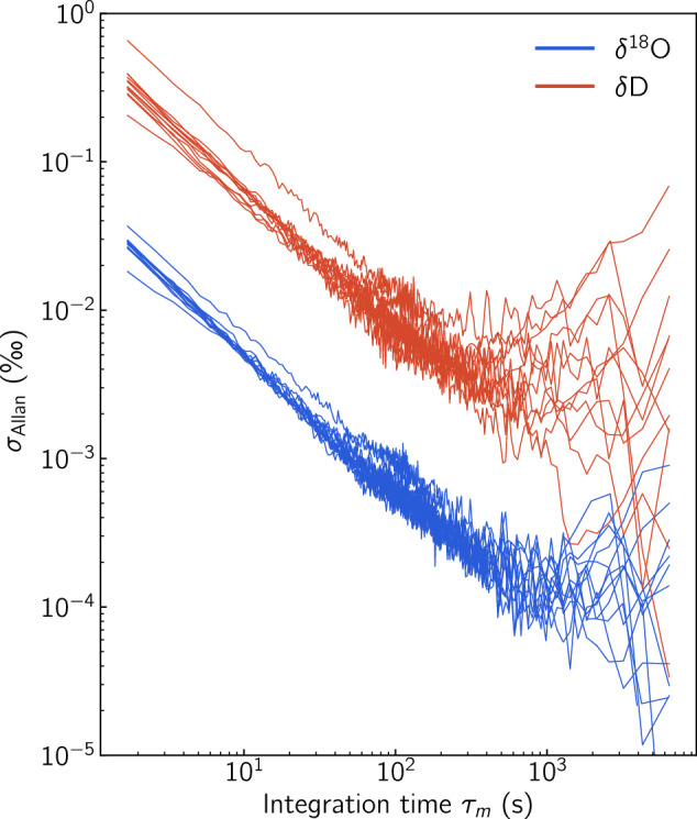
Allan standard deviation as a function of integration time for δ18O and δD. The metrics are based on the overnight Idle sections in the period 10/10/2019-25/10/2019.
VSMOW-SLAP Calibration accuracy
As described in section VSMOW-SLAP calibration the internal accuracy of the system can be estimated from the offset between the calibrated and the nominal value of the middle “check” local standard water that is treated as an unknown. The metrics from the calibration accuracy runs are summarised in Fig. 10. The “check” standard offset is below 0.07 and 0.6 ‰ for δ18O and δD respectively for all 13 VSMOW-SLAP calibration runs during the CFA campaign. The mean value of the offset is 0.034 ± 0.015 ‰ and 0.32 ± 0.11‰ for δ18O and δD respectively.
Fig. 10.

Internal accuracy for the “check” local standard “NEEM” as estimated during the VSMOW-SLAP calibration at the beginning of each analysis day. For δ18O: 0.034 ± 0.015 ‰, and for δD: 0.32 ± 0.11‰.
Power spectral density noise estimation
While the Allan variance and the VSMOW-SLAP accuracy checks are very useful tools in assessing the performance of the system, they cannot account for noise occurring during the measurement of the ice core sample. This noise could be due to instabilities in the liquid sample flow or the melting of the ice core and typically result in the inclusion of air bubbles in the system. These can in turn disturb the continuous vaporisation process yielding a fluctuating [H2O] concentration in the spectrometer’s optical cavity. The large number of data points in the record due to the high resolution, allows for a more pragmatic and direct estimation of the records’ noise levels. Similar to the approach followed in39, the noise of a data section can be deduced from the noise component of the power spectral density (PSD) of the δ18O, δD signals by calculating the integral:
| 9 |
where fc = 1/2Δx = 100 m−1 is the Nyquist frequency. With being the Fourier transform of the δ18O,δD signals, can be estimated by a linear fit on the flat high-frequency part of the power spectral density . For this study, we implement a rolling window with a size of 1000 points and calculate the Discrete Fast Fourier Transform (DFFT) for real-valued data53,54 from which an estimate of the PSD can be obtained. The spectra reveal an easy to identify, white-noise plateau the level of which we obtain by means of a least squares fit of a zero-order polynomial for frequencies higher than 50 m−1. Subsequently we filter the measurement noise signals with a 200 point Gaussian filter. The result of the calculation is given in Fig. 11 revealing a noise level of 0.063 ± 0.008 ‰ and 0.314 ± 0.04‰ for δ18O and δD respectively. Histograms of the measurement noise distributions are also calculated and illustrated in Fig. 12.
Fig. 11.

Measurement noise of the δ18O and δD signals as a function of ice core depth estimated from the noise component of the power spectral density of the isotope signals.
Fig. 12.

Histograms of the CFA measurement noise in Fig. 11. δ18O: 0.063 ± 0.008 ‰, δD: 0.311 ± 0.036‰.
Discrete - CFA comparison
The overlap between the two records in the depth range 93-104 m allows for a comparison between the two datasets. Such a comparison is useful in identifying non systematic errors that typically cannot be characterised using the validation procedures described in the previous sections. Firstly, we average the CFA dataset on the resolution of the discrete samples. The comparison plot overlaying the CFA measurements on the discrete data shows a very good agreement between the time series (Fig. 13) revealing the ice core isotope signal for both δ18O and δD without any outliers or obvious discrepancies. A step further, we plot the signals against each other (Fig. 14) in order to investigate further for possible outliers on both signals. The correlation coefficients derived from this comparisons are 0.989 and 0.988 for δ18O and δD respectively. The plots reveal a number of data points with a relatively high deviation from the correlation line thus showing indication for a non-normal distribution of the measurement errors.
Fig. 13.

A visual comparison between the discrete and the CFA datasets for δ18O and δD. The CFA data are averaged on the resolution of the discrete sampling.
Fig. 14.

Correlation between the discrete and CFA averaged datasets for δ18O and δD. The correlation concerns the depth range 93-104 in which both techniques were used for the isotope analysis and is equal to 0.989 and 0.988 for δ18O and δD respectively.
In order to investigate this we form a hypothesis test using the Shapiro-Wilk statistic55 for departure from normality. In particular, we use a modified version54,56 of the algorithm introduced by Royston57, that is optimised for larger datasets with size 3 ≤ n ≤ 5000. We test the null-hypothesis that the residuals between the two series are distributed normally, by comparing the Shapiro statistic of the data residuals to the statistic of 10,000 realisations of randomly distributed residuals following a Monte Carlo approach. The Shapiro-Wilk statistic yields values closer to 1 for normally distributed variables. The Monte Carlo simulation yields a Shapiro-Wilk statistic equal to 0.969 and 0.944 for the residuals of the δ18O and the δD series respectively (Fig. 15). The p-value for both estimates is below 10−5. This is a very strong indication that the null-hypothesis is false and thus the residuals between the CFA and discrete data are not normally distributed for either of the isotope ratios measured. This result indicates that despite the sound validation procedures for accuracy and precision as well as depth registration, non-systematic sources of error can still exist and go unnoticed. In practical terms, the signal to noise ratio in the isotope signal is so high that the observed discrepancies between the discrete and the CFA data are insignificant.
Fig. 15.
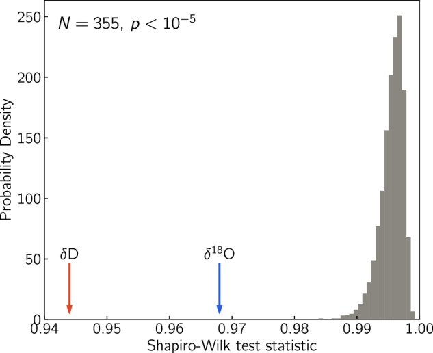
Shapiro-Wilk normality test for the residuals between the CFA and discrete data for δ18O and δD datasets for the depth range 93-104 m. The red and blue arrow signify the value of the Shapiro-Wilk statistic for the δD and δ18O residuals respectively. The gray distribution demonstrates the results of the Monte Carlo simulation using 10000 realisations of a series with N = 355 drawn from a normal distribution. The p-value for both the δD and the δ18O residuals is <10−5 signifying that it is very unlikely that the residuals between the discrete and the CFA data series are normally distributed.
Acknowledgements
This study was supported by the Australian Government’s Antarctic Science Collaboration Initiative (ASCI000002) through funding to the Australian Antarctic Program Partnership. Logistics and analytical funding was provided by an Australian Antarctic Science grant (AAS 4061, 4414 and 4537), the Australian Antarctic Division, the Carlsberg Foundation and a European Union Horizon 2020 research and innovation grant (TiPES, H2020 grant no. 820970). This study contributes to an Australian Research Council (ARC) Discovery Project (DP220100606) to TRV and NJA. NJA was supported by an ARC Future Fellowship (FT160102059), and NJA and SLJ were supported by the ARC Special Research Initiative Australian Centre of Excellence in Antarctic Science (SR200100008) and the Centre of Excellence for Climate Extremes (CE170100023). VG acknowledges funding from the Villum Foundation (Villum Fonden Grant 00022995, 00028061) and the Danish Research Foundation (Grant 10.46540/2032-00228B). HAK acknowledges funding from the Danish Novo Nordic foundation for the project PRECISE. TQ acknowledges funding from the Danish National Research Foundation (Danmarks Grundforskningsfond). We would like to acknowledge significant contributions from Paul Vallelonga in obtaining funding for the drilling operation of the MBS project as well as coordinating the measurement campaigns in Copenhagen.
Author contributions
V.G. designed the system for the CFA water isotope analysis and conducted the measurements during the campaign with S.J., K.M.P. and T.Q. V.G. developed the data analysis and quality validations methods presented in the manuscript. V.G. and S.J. performed the VSMOW-SLAP calibrations, depth registration and further data analysis of the CFA measurements. A.D.M., S.J., C.T.P., N.J.A., and T.R.V. contributed to processing, analysis, dating and interlaboratory comparisons of the discretely sampled isotope data. T.R.V. led the development of the age scale, MBS2023, with primary contributions from C.T.P. and H.A.K. H.A.K., T.B., M.H. and V.G. set up and operated the CFA melting and sample distribution system. H.A.K., A.S. and A.D.M. participated in preparation of the core in the freezer. V.G. and S.J. wrote the manuscript with contributions from N.J.A., H.A.K. and T.R.V.
Code availability
The Python code used for this study is available on GitHub (https://github.com/vgkinis/mbs_cfa_isotopes).
Competing interests
The authors declare no competing interests.
Footnotes
Publisher’s note Springer Nature remains neutral with regard to jurisdictional claims in published maps and institutional affiliations.
References
- 1.EPICA Community Members. Eight glacial cycles from an Antarctic ice core. Nature429, 623–628, 10.1038/nature02599 (2004). 10.1038/nature02599 [DOI] [PubMed] [Google Scholar]
- 2.EPICA Community Members. One-to-one coupling of glacial climate variability in Greenland and Antarctica. Nature444, 195–198, 10.1038/nature05301 (2006). 10.1038/nature05301 [DOI] [PubMed] [Google Scholar]
- 3.WAIS Divide Project Members. Onset of deglacial warming in West Antarctica driven by local orbital forcing. Nature500, 440–446, 10.1038/nature12376 (2013). 10.1038/nature12376 [DOI] [PubMed] [Google Scholar]
- 4.Van Ommen, T. D., Morgan, V. & Curran, M. A. J. Deglacial and Holocene changes in accumulation at Law Dome, East Antarctica. Annals of Glaciology39, 359–365, 10.3189/172756404781814221 (2004). 10.3189/172756404781814221 [DOI] [Google Scholar]
- 5.Roberts, J. et al. A 2000-year annual record of snow accumulation rates for Law Dome, East Antarctica. Clim. Past11, 697–707, 10.5194/cp-11-697-2015 (2015). 10.5194/cp-11-697-2015 [DOI] [Google Scholar]
- 6.Jouzel, J. & Merlivat, L. Deuterium and oxygen 18 in precipitation: modeling of the isotopic effects during snow formation. J. Geophys. Res.-Atmospheres89, 11749 – 11759–11749 – 11759 (1984). 10.1029/JD089iD07p11749 [DOI] [Google Scholar]
- 7.Johnsen, S. J. et al. Oxygen isotope and palaeotemperature records from six Greenland ice-core stations: Camp Century, Dye-3, GRIP, GISP2, Renland and NorthGRIP. Journal Of Quaternary Science16, 299–307–299–307 (2001). 10.1002/jqs.622 [DOI] [Google Scholar]
- 8.Jouzel, J. A brief history of ice core science over the last 50 yr. Clim. Past9, 2525–2547, 10.5194/cp-9-2525-2013 (2013). 10.5194/cp-9-2525-2013 [DOI] [Google Scholar]
- 9.Markle, B. R. & Steig, E. J. Improving temperature reconstructions from ice-core water-isotope records. Clim. Past18, 1321–1368, 10.5194/cp-18-1321-2022 (2022). 10.5194/cp-18-1321-2022 [DOI] [Google Scholar]
- 10.Mook, W. G.Environmental Isotopes in the Hydrological Cycle: Principles and Applications, vol. 1 (IAEA-UNESCO: Paris, France, 2001).
- 11.International Atomic Energy Agency. Reference Sheet for VSMOW2 and SLAP2 International Measurement Standards. Tech. Rep., IAEA, Vienna (2017).
- 12.Vance, T. R. et al. Optimal site selection for a high-resolution ice core record in East Antarctica. Clim. Past12, 595–610, 10.5194/cp-12-595-2016 (2016). 10.5194/cp-12-595-2016 [DOI] [Google Scholar]
- 13.Vance, T. R. et al. An annually resolved chronology for the Mount Brown South ice cores, East Antarctica. Clim. Past20, 969–990, 10.5194/cp-20-969-2024 (2024). 10.5194/cp-20-969-2024 [DOI] [Google Scholar]
- 14.Gkinis, V., Popp, T. J., Johnsen, S. J. & Blunier, T. A continuous stream flash evaporator for the calibration of an IR cavity ring-down spectrometer for the isotopic analysis of water. Isotopes In Environmental and Health Studies46, 463–475, 10.1080/10256016.2010.538052 (2010). 10.1080/10256016.2010.538052 [DOI] [PubMed] [Google Scholar]
- 15.Crockart, C. K. et al. El Niño-Southern Oscillation signal in a new East Antarctic ice core, Mount Brown South. Clim. Past17, 1795–1818, 10.5194/cp-17-1795-2021 (2021). 10.5194/cp-17-1795-2021 [DOI] [Google Scholar]
- 16.Jackson, S. L. et al. Climatology of the Mount Brown South ice core site in East Antarctica: implications for the interpretation of a water isotope record. Clim Past19, 1653–1675, 10.5194/cp-19-1653-2023 (2023). 10.5194/cp-19-1653-2023 [DOI] [Google Scholar]
- 17.Ekaykin, A. A., Vladimirova, D. O., Lipenkov, V. Y. & Masson-Delmotte, V. Climatic variability in Princess Elizabeth Land (East Antarctica) over the last 350 years. Clim. Past13, 61–71, 10.5194/cp-13-61-2017 (2017). 10.5194/cp-13-61-2017 [DOI] [Google Scholar]
- 18.Delmotte, M., Masson, V., Jouzel, J. & Morgan, V. I. A seasonal deuterium excess signal at Law Dome, coastal eastern Antarctica: A southern ocean signature. Journal of Geophysical Research: Atmospheres105, 7187–7197, 10.1029/1999JD901085 (2000). 10.1029/1999JD901085 [DOI] [Google Scholar]
- 19.Stenni, B. et al. Antarctic climate variability on regional and continental scales over the last 2000 years. Clim. Past13, 1609–1634–1609–1634, 10.5194/cp-13-1609-2017 (2017). 10.5194/cp-13-1609-2017 [DOI] [Google Scholar]
- 20.Zheng, Y. et al. Extending and understanding the South West Western Australian rainfall record using a snowfall reconstruction from Law Dome, East Antarctica. Clim. Past17, 1973–1987, 10.5194/cp-17-1973-2021 (2021). 10.5194/cp-17-1973-2021 [DOI] [Google Scholar]
- 21.van Ommen, T. D. & Morgan, V. Snowfall increase in coastal East Antarctica linked with southwest Western Australian drought. Nature Geoscience3, 267–272, 10.1038/ngeo761 (2010). 10.1038/ngeo761 [DOI] [Google Scholar]
- 22.Vance, T. R., Roberts, J. L., Plummer, C. T., Kiem, A. S. & van Ommen, T. D. Interdecadal Pacific variability and eastern Australian megadroughts over the last millennium. Geophys. Res. Lett.42, 129–137, 10.1002/2014GL062447 (2015). 10.1002/2014GL062447 [DOI] [Google Scholar]
- 23.Vance, T. R. et al. Pacific decadal variability over the last 2000 years and implications for climatic risk. Commun. Earth Environ.3, 33, 10.1038/s43247-022-00359-z (2022). 10.1038/s43247-022-00359-z [DOI] [Google Scholar]
- 24.Udy, D. G., Vance, T. R., Kiem, A. S. & Holbrook, N. J. A synoptic bridge linking sea salt aerosol concentrations in East Antarctic snowfall to Australian rainfall. Commun. Earth Environ.3, 175, 10.1038/s43247-022-00502-w (2022). 10.1038/s43247-022-00502-w [DOI] [Google Scholar]
- 25.Johnsen, S. J. et al. The Hans Tausen drill: design, performance, further developments and some lessons learned. Annals of Glaciology47, 89–98, 10.3189/172756407786857686 (2007). 10.3189/172756407786857686 [DOI] [Google Scholar]
- 26.Sigg, A., Fuhrer, K., Anklin, M., Staffelbach, T. & Zurmuhle, D. A Continuous Analysis Technique For Trace Species In Ice Cores. Environ. Sci. Technol.28, 204–209–204–209 (1994). 10.1021/es00051a004 [DOI] [PubMed] [Google Scholar]
- 27.Röthlisberger, R. et al. Technique for continuous high-resolution analysis of trace substances in firn and ice cores. Environ. Sci. Technol.34, 338–342–338–342 (2000). 10.1021/es9907055 [DOI] [Google Scholar]
- 28.Kaufmann, P. R. et al. An Improved Continuous Flow Analysis System for High-Resolution Field Measurements on Ice Cores. Environ. Sci. Technol.42, 8044–8050–8044–8050 (2008). 10.1021/es8007722 [DOI] [PubMed] [Google Scholar]
- 29.Bigler, M. et al. Optimization of High-Resolution Continuous Flow Analysis for Transient Climate Signals in Ice Cores. Environ. Sci. Technol.45, 4483–4489–4483–4489, 10.1021/es200118j (2011). 10.1021/es200118j [DOI] [PubMed] [Google Scholar]
- 30.Sigl, M. et al. A new bipolar ice core record of volcanism from WAIS Divide and NEEM and implications for climate forcing of the last 2000 years. J. Geophys. Res. Atmos.118, 1151–1169–1151–1169 (2013). 10.1029/2012JD018603 [DOI] [Google Scholar]
- 31.Sigl, M. et al. The WAIS Divide deep ice core WD2014 chronology - Part 2: Annual-layer counting (0-31 ka BP). Clim. Past12, 769–786, 10.5194/cp-12-769-2016 (2016). 10.5194/cp-12-769-2016 [DOI] [Google Scholar]
- 32.Simonsen, M. F. et al. East Greenland ice core dust record reveals timing of Greenland ice sheet advance and retreat. Nature Communications10, 4494, 10.1038/s41467-019-12546-2 (2019). 10.1038/s41467-019-12546-2 [DOI] [PMC free article] [PubMed] [Google Scholar]
- 33.Erhardt, T. et al. High-resolution aerosol concentration data from the Greenland NorthGRIP and NEEM deep ice cores. Earth Syst. Sci. Data14, 1215–1231, 10.5194/essd-14-1215-2022 (2022). 10.5194/essd-14-1215-2022 [DOI] [Google Scholar]
- 34.Crosson, E. R. A cavity ring-down analyzer for measuring atmospheric levels of methane, carbon dioxide, and water vapor. Applied Physics B-Lasers And Optics92, 403–408, 10.1063/1.1139895 (2008). 10.1063/1.1139895 [DOI] [Google Scholar]
- 35.Gupta, P., Noone, D., Galewsky, J., Sweeney, C. & Vaughn, B. H. Demonstration of high-precision continuous measurements of water vapor isotopologues in laboratory and remote field deployments using wavelength-scanned cavity ring-down spectroscopy (ws-crds) technology. Rapid Communications In Mass Spectrometry23, 2534–2542 (2009). 10.1002/rcm.4100 [DOI] [PubMed] [Google Scholar]
- 36.Steig, E. J. et al. Calibrated high-precision 17O-excess measurements using cavity ring-down spectroscopy with laser-current-tuned cavity resonance. Atmos. Meas. Tech.7, 2421–2435 (2014). 10.5194/amt-7-2421-2014 [DOI] [Google Scholar]
- 37.Stowasser, C. et al. Continuous measurements of methane mixing ratios from ice cores. Atmos. Meas. Tech. Techniques5, 999–1013–999–1013, 10.5194/amt-5-999-2012 (2012). 10.5194/amt-5-999-2012 [DOI] [Google Scholar]
- 38.Rhodes, R. H. et al. Continuous methane measurements from a late holocene greenland ice core: Atmospheric and in-situ signals. Earth and Planetary Science Letters368, 9–19–9–19 (2013). 10.1016/j.epsl.2013.02.034 [DOI] [Google Scholar]
- 39.Gkinis, V. et al. Water isotopic ratios from a continuously melted ice core sample. Atmos. Meas. Tech.4, 2531–2542, 10.5194/amt-4-2531-2011 (2011). 10.5194/amt-4-2531-2011 [DOI] [Google Scholar]
- 40.Emanuelsson, B. D., Baisden, W. T., Bertler, N. A. N., Keller, E. D. & Gkinis, V. High-resolution continuous-flow analysis setup for water isotopic measurement from ice cores using laser spectroscopy. Atmos. Meas. Tech.8, 2869–2883, 10.5194/amt-8-2869-2015 (2015). 10.5194/amt-8-2869-2015 [DOI] [Google Scholar]
- 41.Jones, T. R. et al. Improved methodologies for continuous-flow analysis of stable water isotopes in ice cores. Atmos. Meas. Tech.10, 617–632, 10.5194/amt-10-617-2017 (2017). 10.5194/amt-10-617-2017 [DOI] [Google Scholar]
- 42.Steig, E. J. et al. Continuous-Flow Analysis of δ17O, δ18O, and δD of H2O on an Ice Core from the South Pole. Front. Earth Sci.9, 640292, 10.3389/feart.2021.640292 (2021). 10.3389/feart.2021.640292 [DOI] [Google Scholar]
- 43.Kjær, H. A. et al. Canadian forest fires, icelandic volcanoes and increased local dust observed in six shallow greenland firn cores. CP18, 2211–2230, 10.5194/cp-18-2211-2022 (2022). 10.5194/cp-18-2211-2022 [DOI] [Google Scholar]
- 44.Harlan, M. et al. 1137 years of high-resolution Continuous Flow Analysis impurity data from the Mount Brown South Ice Core, Ver. 1. Australian Antarctic Data Centre10.26179/9tke-0s16 (2024). 10.26179/9tke-0s16 [DOI]
- 45.Hughes, A. G. et al. High-frequency climate variability in the Holocene from a coastal-dome ice core in east-central Greenland. Clim. Past16, 1369–1386, 10.5194/cp-16-1369-2020 (2020). 10.5194/cp-16-1369-2020 [DOI] [Google Scholar]
- 46.Werle, P. Accuracy and precision of laser spectrometers for trace gas sensing in the presence of optical fringes and atmospheric turbulence. Applied Physics B-lasers and Optics102, 313–329–313–329, 10.1007/s00340-010-4165-9 (2011). 10.1007/s00340-010-4165-9 [DOI] [Google Scholar]
- 47.Vance, T. R. et al. MBS2023 - The Mount Brown South ice core chronologies and chemistry data, Ver. 1. Australian Antarctic Data Centre10.26179/352b-6298 (2024). 10.26179/352b-6298 [DOI]
- 48.Jong, L. M. et al. 2000 years of annual ice core data from Law Dome, East Antarctica. Earth Syst. Sci. Data14, 3313–3328, 10.5194/essd-14-3313-2022 (2022). 10.5194/essd-14-3313-2022 [DOI] [Google Scholar]
- 49.Winstrup, M. et al. A 2700-year annual timescale and accumulation history for an ice core from Roosevelt Island, West Antarctica. Clim. Past15, 751–779, 10.5194/cp-15-751-2019 (2019). 10.5194/cp-15-751-2019 [DOI] [Google Scholar]
- 50.Plummer, C. T. et al. An independently dated 2000-yr volcanic record from Law Dome, East Antarctica, including a new perspective on the dating of the 1450s CE eruption of Kuwae, Vanuatu. Clim. Past8, 1929–1940, 10.5194/cp-8-1929-2012 (2012). 10.5194/cp-8-1929-2012 [DOI] [Google Scholar]
- 51.Gkinis, V. et al. An 1135 year very high-resolution water isotope record of polar precipitation from the Indo-Pacific sector of East Antarctica. Australian Antarctic Data Centre10.26179/ygeq-1a95 (2024). 10.26179/ygeq-1a95 [DOI]
- 52.Werle, P., Mucke, R. & Slemr, F. The limits of signal averaging in atmospheric trace-gas monitoring by tunable diode-laser absorption-spectroscopy (tdlas). Applied Physics B-Photophysics And Laser Chemistry57, 131–139–131–139 (1993). 10.1007/BF00425997 [DOI] [Google Scholar]
- 53.Kay, S. M. & Marple, S. L. Spectrum Analysis - A Modern Perspective. Proceedings Of The IEEE69, 1380–1419–1380–1419 (1981). 10.1109/PROC.1981.12184 [DOI] [Google Scholar]
- 54.Virtanen, P. et al. SciPy 1.0: Fundamental Algorithms for Scientific Computing in Python. Nature Methods17, 261–272, 10.1038/s41592-019-0686-2 (2020). 10.1038/s41592-019-0686-2 [DOI] [PMC free article] [PubMed] [Google Scholar]
- 55.Shapiro, S. S. & Wilk, M. B. An Analysis of Variance Test for Normality (Complete Samples). Biometrika52, 591–611, 10.2307/2333709 (1965). 10.2307/2333709 [DOI] [Google Scholar]
- 56.Royston, P. Remark AS R94: A Remark on Algorithm AS 181: The W-test for Normality. Journal of the Royal Statistical Society. Series C (Applied Statistics)44, 547–551, 10.2307/2986146 (1995). 10.2307/2986146 [DOI] [Google Scholar]
- 57.Royston, J. P. Algorithm AS 181: The W Test for Normality. Journal of the Royal Statistical Society. Series C (Applied Statistics)31, 176–180, 10.2307/2347986 (1982). 10.2307/2347986 [DOI] [Google Scholar]
Associated Data
This section collects any data citations, data availability statements, or supplementary materials included in this article.
Data Citations
- Harlan, M. et al. 1137 years of high-resolution Continuous Flow Analysis impurity data from the Mount Brown South Ice Core, Ver. 1. Australian Antarctic Data Centre10.26179/9tke-0s16 (2024). 10.26179/9tke-0s16 [DOI]
- Vance, T. R. et al. MBS2023 - The Mount Brown South ice core chronologies and chemistry data, Ver. 1. Australian Antarctic Data Centre10.26179/352b-6298 (2024). 10.26179/352b-6298 [DOI]
- Gkinis, V. et al. An 1135 year very high-resolution water isotope record of polar precipitation from the Indo-Pacific sector of East Antarctica. Australian Antarctic Data Centre10.26179/ygeq-1a95 (2024). 10.26179/ygeq-1a95 [DOI]
Data Availability Statement
The Python code used for this study is available on GitHub (https://github.com/vgkinis/mbs_cfa_isotopes).