Abstract
Plastic particle pollution has threatened the well-being of seawater ecosystems over the past decades. Therefore, understanding, modeling and (potentially) predicting the dynamics of microplastics and biogenic particles in ocean turbulence is of utmost importance to help develop mitigation strategies and propose technological solutions ultimately aimed at safeguarding global water systems. This is particularly significant for microplastics in the upper-ocean layer. To that end, this work presents a comprehensive and openly accessible dataset carefully designed to explore the interplay between the flow physics of particle-laden turbulence and the physicochemical effects of biofilm stickiness. The dataset comprises nine point-particle direct numerical simulations of fluid flow featuring microplastic and biogenic debris within a periodic three-dimensional flow domain. In all cases, the chosen turbulent intensity and microparticle properties represent conditions observed in the upper-ocean layer. This data repository aims to facilitate in-depth exploration, modeling and prediction of the intricate flow physics observed in marine microplastics, particularly regarding their distribution and aggregation.
Keywords: Aggregation, Direct numerical simulation, Microplastics, Ocean turbulence, Particle-laden flow
Specifications Table
| Subject | Physics |
| Specific subject area | Fluid mechanics |
| Type of data | Tables (csv format); Raw, Filtered data; Code & Scripts. |
| Data collection | A total of 9 simulation runs are acquired through high fidelity direct numerical simulations (DNS). The numerical domain represents an upper-ocean cubic region based on homogeneous isotropic turbulence, along with a bidisperse mixture of point particles representing microplastics and biogenic material. The adopted mesh ensures full resolution of all turbulent scales, and the particle sizes align with literature data. The dataset includes the instantaneous flow velocity field over time, as well as the positions and velocities of the particles. Additionally, the aggregates are computed as a post-process. |
| Data source location | Dept. Fluid Mechanics, Barcelona East School of Engineering, Universitat Politècnica de Catalunya ‧ BarcelonaTech (UPC), Barcelona, Spain |
| Data accessibility | Repository name: Figshare+ Data identification number: https://doi.org/10.25452/figshare.plus.25498372 Direct URL to data: https://plus.figshare.com/articles/dataset/ Distribution_and_Aggregation_of_Microparticles_in_Upper-Ocean_Turbulence_Dataset/25498372 Instructions: Data are openly accessible and available for download |
| Related research article | None |
1. Value of the Data
-
•
This dataset empowers researchers to explore the intricate behavior of microplastic (MP) and biogenic particles (BPs) in the turbulent upper region of oceans through point-particle direct numerical simulation data. It provides time-series data of fully-resolved turbulent flow fields and Lagrangian points which represent the marine debris, facilitating comprehensive analysis and the development of models to predict the fate of microplastics.
-
•
The 9 simulation cases provided, spanning a wide range of particle properties and stickiness characteristics, will be valuable to an interdisciplinary audience including physicists and engineers specialized in fluid mechanics, as well as environmental scientists.
-
•
The innovative integration of physical properties (such as turbulence and particle size) with physicochemical characteristics (e.g., coagulation efficiency) of marine debris enables the calculation of parameters such as particles preferential concentration and distribution, aggregates formation and composition, and the tracking of particle trajectories and collisions.
2. Background
The proliferation and impact of marine microplastics, plastic pieces smaller than 5 millimeters, are a growing concern within the realm of environmental science and marine biology [1]. Recent estimations reveal an astonishing presence of plastic debris in the ocean [2], which engage with marine ecosystems [3]. A significant challenge is understanding the fate of “missing plastic”: only 1% of the plastic entering the ocean annually is observed floating at the surface [4]. The prevailing hypothesis attributes this scarcity to the sinking of light plastic debris to deeper layers of the ocean [5] due to the aggregation with biogenic material [5,6]. Nonetheless, examining the aggregation processes of particles in upper-ocean turbulence is particularly challenging due to the complex nature of the problem, involving a multitude of particles, turbulent flow and diverse biophysical properties.
Therefore, motivated by the limited research data available and the growing scientific interest in microplastic behavior in ocean environments, this work is dedicated to present a curated dataset of DNSs comprising 9 particle-laden turbulent cases. By doing so, researchers can pinpoint the precise factors influencing microplastics movement and aggregation, paving the way for more accurate predictive models and helping to develop mitigation strategies.
3. Data Description
3.1. Dataset hierarchy
The data and post-processing scripts are available as an open dataset [7] on Figshare+ [8]. The 9 different simulations, whose main features are summarized in Table 1, are organized systematically to facilitate access and analysis. The various simulations are characterized by the following properties: for cases 1, 2, 3 and 7, 8, 9, simulations are advanced for five Taylor microscale times (as listed in Table 5), while for cases 4, 5, 6, which contain a significantly large number of particles incurring high computational costs, are advanced for one Taylor microscale time. Such relatively short simulation time is a consequence of the expensive detection of particle-particle collisions algorithm, which as a result imply that particles: (i) do not completely experience the full turbulent spectrum, particularly the large flow scales; and (ii) the effects of gravity become less important as described in Section 4.2. Finally, the parameter that determines whether coalescence occurs upon collision is the stickiness parameter, viz. the probability of particles to attach upon collision events (also defined as coagulation efficiency, α) [9,10]. The simulations conducted consider three values of stickiness (α = 1/3, 2/3, 3/3) for three different cases of microparticle combinations (see Table 1).
Table 1.
Summary of input parameters and corresponding dimensionless numbers of the simulations presented in the database. In detail: dp1 represents the diameter of microplastics, dp2 is the diameter of biogenic particles, np1 denotes the number density of microplastics, np2 indicates the number density of biogenic particles; Stλ1 is the Stokes number for microplastics, Stλ2 is the Stokes number for biogenic particles; Φv represents the mixture volume fraction, and α is the coagulation efficiency. For a comprehensive description of these parameters, refer to Section 4.
| Case | dp1 [m] | dp2 [m] | np1 [prt/m3] | np2 [prt/m3] | Stλ1 | Stλ2 | Φv | α |
|---|---|---|---|---|---|---|---|---|
| 1 | 1.5‧10−4 | 7.5‧10−5 | 1.0‧107 | 1.0‧107 | 1.92‧10−4 | 7.20‧10−5 | 1.99‧10−5 | 1/3 |
| 2 | 1.5‧10−4 | 7.5‧10−5 | 1.0‧107 | 1.0‧107 | 1.92‧10−4 | 7.20‧10−5 | 1.99‧10−5 | 2/3 |
| 3 | 1.5‧10−4 | 7.5‧10−5 | 1.0‧107 | 1.0‧107 | 1.92‧10−4 | 7.20‧10−5 | 1.99‧10−5 | 3/3 |
| 4 | 1.5‧10−4 | 7.5‧10−5 | 2.5‧107 | 5.0‧107 | 1.92‧10−4 | 7.20‧10−5 | 5.52‧10−5 | 1/3 |
| 5 | 1.5‧10−4 | 7.5‧10−5 | 2.5‧107 | 5.0‧107 | 1.92‧10−4 | 7.20‧10−5 | 5.52‧10−5 | 2/3 |
| 6 | 1.5‧10−4 | 7.5‧10−5 | 2.5‧107 | 5.0‧107 | 1.92‧10−4 | 7.20‧10−5 | 5.52‧10−5 | 3/3 |
| 7 | 3.0‧10−4 | 1.5‧10−4 | 1.0‧107 | 1.0‧107 | 7.68‧10−4 | 2.90‧10−4 | 1.59‧10−5 | 1/3 |
| 8 | 3.0‧10−4 | 1.5‧10−4 | 1.0‧107 | 1.0‧107 | 7.68‧10−4 | 2.90‧10−4 | 1.59‧10−5 | 2/3 |
| 9 | 3.0‧10−4 | 1.5‧10−4 | 1.0‧107 | 1.0‧107 | 7.68‧10−4 | 2.90‧10−4 | 1.59‧10−5 | 3/3 |
Table 5.
Main timescales of the problem: τλ denotes the Taylor microscale time, τη represents the Kolmogorov timescale, and τp1 & τs1 and τp2 & τs2 are the relaxation and settling timescales of microplastics and biogenic particles, respectively. Values in line with Ref. [18].
| Timescales | τλ [s] | τη [s] | τp1 [s] | τp2 [s] | τs1 [s] | τs2 [s] |
|---|---|---|---|---|---|---|
| Values | 4.6 | 1.2 | [4.9: 35] ‧10−4 | [3.3: 13] ‧10−5 | [3.1: 13] ‧101 | [6.4 : 25] |
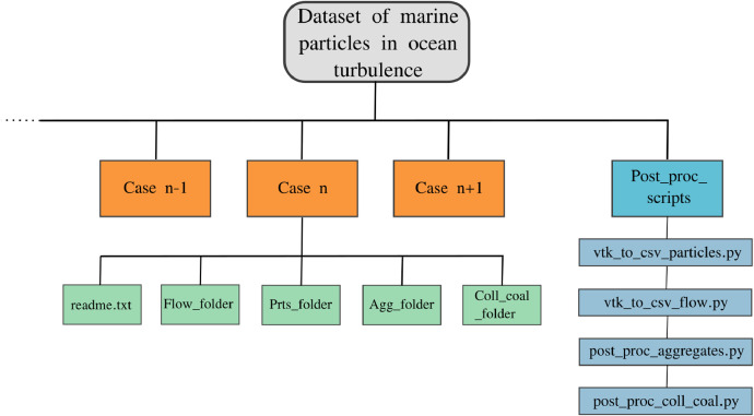
As shown schematically in Fig. 1, each case is stored in a dedicated folder (orange boxes) that, in turn, includes subfolders dedicated to the flow field, particles and aggregates data. Each subfolder contains 50 (cases 1, 2, 3 and 7, 8, 9) or 10 (cases 4, 5, 6) instantaneous snapshots uniformly spaced in time. As specified in Table 2, the flow data (in csv format, named flow_n.csv where n is the ordering number, and located in Flow_folder) includes the x, y, and z velocities (pre-multiplied by the fluid density) and their corresponding coordinates. Table 3 details the properties of the csv particle files (located in Prts_folder and named prt_t_n.csv), which include the x, y, z velocities, the particle class (1 for microplastic or 2 for biogenic particles), and the x, y, z positions. These output variables represent essential parameters directly produced by the simulations, serving as crucial inputs for computing other derived properties.
Fig. 1.
Schematic representing the hierarchical format of the database files. The orange boxes are representative of the 9 cases and for each case the flow, particles, aggregates and collision-coalescence events are stored.
Table 2.
Flow phase variables corresponding to the entry columns of the flow data file included in Flow_folder (see Fig. 1). The second column corresponds to the name of the solver output variable printed in the csv files.
| Variable | SOLEIL quantity | Symbol | Units |
|---|---|---|---|
| x-velocity | Rho-U_X | ρfux | kg/(s‧m2) |
| y-velocity | Rho-U_Y | ρfuy | kg/(s‧m2) |
| z-velocity | Rho-U_Z | ρfuz | kg/(s‧m2) |
| x-coordinate | X | x | m |
| y-coordinate | Y | y | m |
| z-coordinate | Z | z | m |
Table 3.
Particles phase variables corresponding to the entry columns of the particle data files included in Prts_folder (see Fig. 1).
| Variable | SOLEIL quantity | Symbol | Units |
|---|---|---|---|
| x-velocity | Vel : 0 | ux | m/s |
| y-velocity | Vel : 1 | uy | m/s |
| z-velocity | Vel : 2 | uz | m/s |
| Class | dID | - | - |
| x-coordinate | X | xp | m |
| y-coordinate | Y | yp | m |
| z-coordinate | Z | zp | m |
On the other hand, as described in Table 4, the post-processed quantities include the properties of the aggregates, such as their composition (i.e., the number of original microplastics and/or biogenic particles), diameter, density, position & velocity.
Table 4.
List of output (post-processed) aggregate properties/quantities corresponding to the entry columns of the particle data files included in Agg_folder (see Fig. 1).
| Description | Field label | Symbol | Units |
|---|---|---|---|
| MPs content | Number prts. 1 | - | - |
| BPs content | Number prts. 2 | - | - |
| Diameter | Aggregate diameter | dagg | m |
| Density | Aggregate density | ρagg | kg/m3 |
| x-coordinate | x | xagg | m |
| y-coordinate | y | yagg | m |
| z-coordinate | z | zagg | m |
| x-velocity | u | uagg(x) | m/s |
| y-velocity | v | uagg(y) | m/s |
| z-velocity | w | uagg(z) | m/s |
The files containing the information of aggregates, in csv format, are stored in Agg_folder and generated as part of a post-processing routine, which is implemented in the Python file post_proc_aggregates.py (see Fig. 1). In fact, although the particle-flow solver detects and evolves the dynamics of the aggregates through its aggregation kernel, it does not print out the identification or properties of the aggregates. Instead, the solver reports the location and the velocity of all particles, associated to their original identification, even if they are in an aggregate. This is why the particle files presented in Prts_folder contain the same number of rows (viz. particles) for the entire simulation time. Identification of the particles that are in an aggregate at any time can be inferred in the post-processing steps from the overlapping positions of particles reported by the solver. For better clarity, the data for original particles is stored in Prts_folder, and the data for aggregates in the dedicated folder Agg_folder. Moreover, an additional subfolder, named Coll_coal_folder, includes the simulation status file that outlines the temporal progression of collision and coalescence events at each time step. Finally, the simulation setup properties, such as (i) main independent parameters, (ii) dimensionless parameters, and (iii) data saving format, are described in the README.txt file of each case folder.
3.2. Usage notes
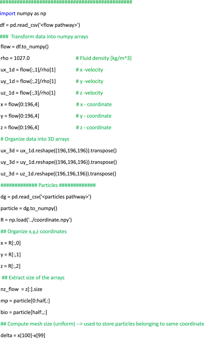
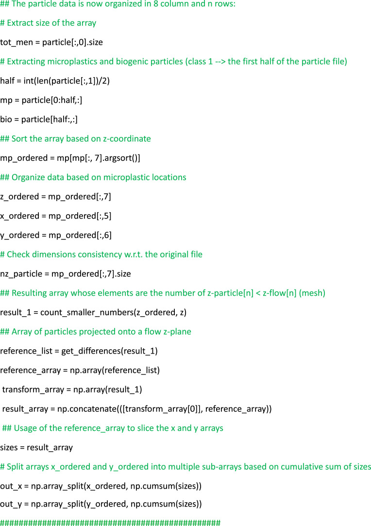
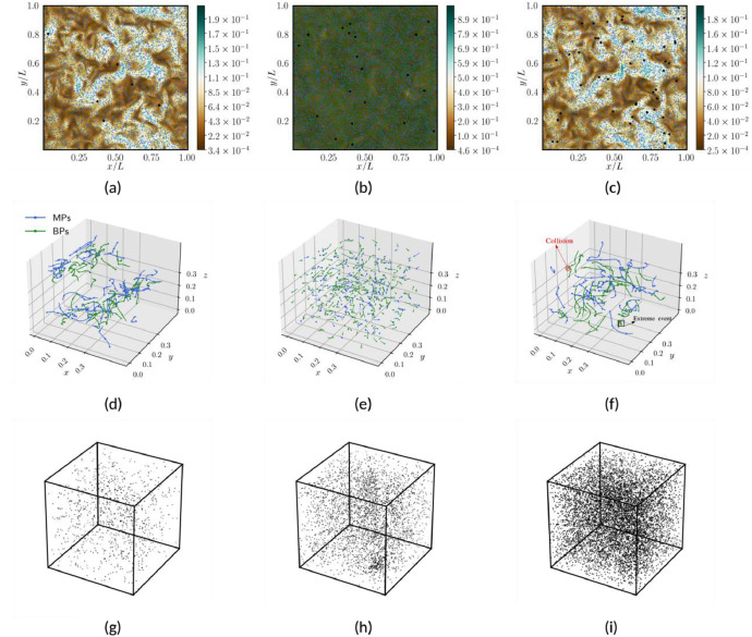
The structured dataset is crafted for user-friendly access, offering readily available data for the instantaneous flow, particles and aggregates files, all stored in csv format. It is important to remark that both microplastic and biogenic particles, as well as their aggregates, are modeled as spherical debris. This simplification enables a greater focus on the overall statistics of marine debris. In detail, each flow file comprises velocity arrays with 196×196×196 data points equally spaced within a periodic domain. The mesh coordinates are labeled as (X, Y, Z) which refer to x, y, and z directions, respectively, as illustrated in Table 4. In terms of particle files, the size of the arrays differs: Cases 1, 2, 3, 7, 8, and 9 consist of 2.5‧106 particles each (corresponding to the number of rows in each file), whereas Cases 4, 5, and 6 contain 9.375‧106 particles each; detailed information about the files are contained in the readme.txt file (see Fig. 1). The comprehensive storage of flow and particle data enables the investigation of complex particle-laden turbulent phenomena. As an example, the user can visualize the particles distribution with respect to the local turbulent intensity as depicted in Figs. 2(a), (b) and (c). For these plots, it is also provided an example of the Python code (see Listing 1) that: (i) reads the flow data and stores them in 3D arrays corresponding to the mesh grid, and (ii) reads the particle data and stores them in z-slices with thickness matching the mesh size. Once this is done, the arrays are ready for plotting. Moreover, the particles output is consistently organized over time, meaning that the particular row of each file corresponds to the same particle. This data setup allows the tracking of particles/aggregates during post-processing analyses, as exemplified in Figs. 2(d), (e) and (f). Such coherence proves highly advantageous as it allows for the examination of geometric properties, visualization of collisions and detection of extreme events, such as small spiral motions of particle trajectories within ocean turbulence. The aggregated files, stored in the Agg_folder in csv format, are generated using an optimized algorithm written in Python language named post_proc_aggregates.py (see Fig. 1). The algorithm used to distinguish aggregates from the original particles is based on basic geometrical considerations and the box-counting method: (i) The box-counting method subdivides the domain into N boxes (6×6×6=216 boxes have been used). For each box, the program checks whether particles are sufficiently close to each other within that subdomain. This approach reduces time consumption since aggregation is a local phenomenon, making it redundant to analyze distances between particles in different boxes. (ii) Once the Euclidean distance between the centers of particle pairs is computed, it is compared to a small threshold value. If the distance is less than this threshold, the aggregate is recorded with a diameter corresponding to (dp13+ dp23)1/3 and the same operation for density. Aggregates can be visualized such as in Figs. 2(g), (h), (i), or analyzed in a more complex fashion in terms of their dynamics and composition [6].
List 1.
Example of post-processing Python script to read, organize, and plot instantaneous flow and particle data to produce plots similar to Fig. 2(a, b, c).
Fig. 2.
Illustrative post-processed outputs from simulations corresponding to Case 3 (left column), Case 6 (center column) and Case 9 (right column). Plots (a), (b) and (c) depict snapshots of turbulent kinetic energy of the flow, where microplastics, biogenic particles and aggregates are represented as blue, green, and black dots, respectively. Plots (d), (e) and (f) exhibit three-dimensional trajectories of various selected particles/aggregates. Finally plots (g), (h) and (I) showcase snapshots of the aggregates within the 3D domain.
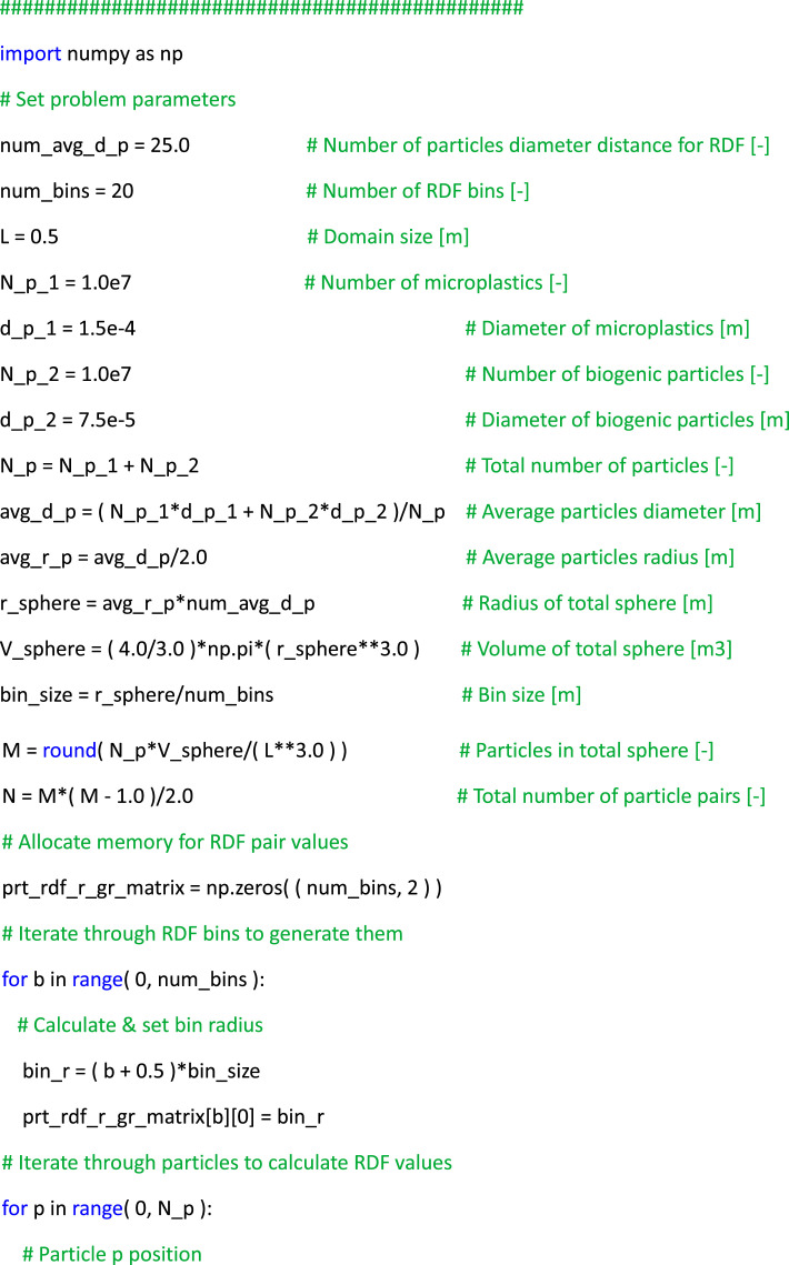
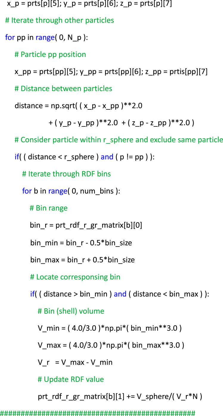
Finally, an illustrative example of utilizing the dataset to compute the radial distribution function (RDF) of particles, a common metric in particle-laden turbulence used to quantify the preferential concentration of the dispersed phase [13], is showcased. In particular, RDFs can be computed for a set of M particles by grouping them based on their separation distance with respect to an isotropic distribution as g(r) = (Nr / Vr) / (N / V), where Nr represents the number of particle pairs within a spherical volume element Vr with radius r from a given test particle location, N = M(M-1)/2 denotes the total number of particle pairs within the volume, and V signifies the total volume. Listing 2 provides a simple example of a Python script to calculate the RDF of particles, which is based on computing the volume of spherical shells around each particle and comparing it to an ideal isotropic distribution. This example serves as a practical demonstration of effectively utilizing the particle data for theoretical analyses.
List 2.
Example of post-processing Python script to read the particle data files and calculate the radial distribution function.
4. Experimental Design, Materials and Methods
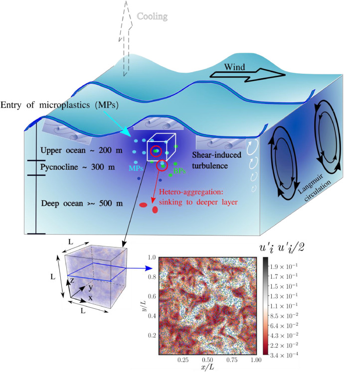
In order to analyze the intricate phenomena of microparticles in oceans, DNS results prove particularly useful as they (i) enable a deep and sophisticated analysis, and (ii) provide access to detailed information of the physics involved. In this regard, the characteristics and strength of oceanic turbulence can vary significantly across different depths, and involve a wide number of processes, as represented in Fig. 3. This work focuses on a small box in the upper-ocean layer which is simulated by means of homogeneous isotropic turbulence (HIT), and neglecting the large-scale shear effects. Under such conditions, marine microplastics can be viewed as an exemplary instance of particle-laden turbulence, wherein turbulent ocean currents (carrier phase) interact with particles (dispersed phase) [9]. Due to the significant separation between flow and particle scales, the representation of microplastics and biogenic material as point particles is motivated by their considerably smaller size compared to the smallest (Kolmogorov) turbulent flow scales.
Fig. 3.
Overview of the primary mechanisms and modeling approach utilized to describe microplastics and biogenic particles in upper-ocean turbulence. The schematic depicts the studied periodic cube containing particles, together with a x-y slice visualizing turbulent flow fluctuations and particles distribution. In this representation, biogenic particles are denoted by green points, while microplastics are represented by blue points.
For this reason, the point-particle (PP) Langrangian-Eulerian (LE) DNS approach is the most natural choice to conduct this type of simulations. In this scenario, particles can be described as Np small Lagrangian points whose masses are defined as mp = (π/6) ρpd3p, with ρp and dp denoting their densities and diameters, respectively. Under this premise, the following subsections will focus on the mathematical modeling of the carrier phase, particle description in terms of dynamics and coagulation effects, and finally, the numerical methods utilized for the simulations.
4.1. Eulerian description of turbulent flow
Under the assumptions of isothermal, incompressible flow conditions, and by choosing the fluid density ρf, dynamic viscosity μf, Taylor microscale λ, and root-mean-square velocity fluctuations Urms as scaling parameters [11], the dimensionless continuity and Navier-Stokes equations read [12]
| (1) |
| (2) |
where and are, respectively, the dimensionless fluid velocity and pressure, and Reλ = λUrms /νf is the Taylor Reynolds number with νf being the kinematic viscosity of the fluid. represents the normalized forcing term that maintains turbulence at the desired Reynolds number [17]. Further details about this added term are provided in subsection 4.3. The term fTWC corresponds to the two-way coupling term representing the effect of particle forces on the fluid, defined as [9]
| (3) |
with being the dimensionless fluid velocity at particle locations and is the particle velocity, Ns the number of particle classes, and the Dirac delta function concentrated at the particle positions. The two-way coupling effect is crucial for particle motion (influencing particle dynamics) and for modulating turbulence. However, in dilute suspensions, such as in the current dataset, this effect is virtually negligible [13]. Defining the flow and particles relaxation times as τλ = λ/Urms and τp = ρpd2p/(18 μf), respectively, the Stokes number Stλ = τp/τλ based on the Taylor microscale is obtained. Finally, Φm= ρpΦv/ρf is the mass fraction of particles in the fluid, with Φv = Np mp /(ρp L3) being the corresponding volume fraction.
4.2. Lagrangian representation of particles and coagulation efficiency
Consistent with typical conditions encountered in marine environments, particles and aggregates in their early stages of formation are significantly smaller than the Kolmogorov flow scale η = (ν3f / ε)1/4 (where ε is the rate of dissipation of turbulent kinetic energy), i.e., dp/η << 1. Furthermore, the influence of settling/rising velocity is neglected as a modeling hypothesis due to the relatively short simulation times compared to the settling time scale τs = λ/Us, where Us = (1 - β) g is the settling velocity with g the gravitational force and β = 3/(2(ρp /ρf)+1) [13] (see Table 5). Moreover, following the values described in the literature [7], the density ratios between particles and fluid are fixed to ρp /ρf = 0.97 for microplastics and ρp /ρf = 1.46 for biogenic particles. Particles are consequently modeled following a Lagrangian PP approach in which Stokes' drag is the most important force. This assumption is asymptotically valid in the limit in which particles are dense with respect to the fluid. Otherwise, the history force of particles needs to be considered. However, (i) becomes important only when ρp /ρf < 10 [13], (ii) has been reported to scale as [10], and (iii) typically presents relatively small impacts on the distribution of particles. As a result, Stokes' drag is the force retained and the description of particles in terms of dimensionless positions and velocities is given by
| (4) |
| (5) |
Particularly, in this work, it is assumed that the particles forming an aggregate are assembled into a spherical, packed configuration, and the resultant aggregate follows the Lagrangian PP equations of motion and collision given by (4)-(5). The density of the aggregate is computed as ρagg = Σp mp / Σp Vp and its diameter is calculated as dagg = (Σp d3p)1/3, where the sums are over all the particles composing the aggregate. Moreover, in the context of PP approximations, interactions between particles are usually characterized using collision models that rely on the conservation of total momentum and energy [6]. The collision dynamics (also referred to as four-way coupling [13]) is described using kinetic models that rely on the equilibrium of overall momentum and energy. Specifically, when two particles (or aggregates) labelled as 1 and 2 engage in a collision, the post-collision (PC) velocities and are related to the before-collision (BC) ones as [6]
| (6) |
| (7) |
where and denote the velocities of the particles before the collision, with CR being the restitution coefficient. The extremes of CR correspond to scenarios where the particles merge upon impact (0, indicating a perfectly inelastic collision), or rebound with the same relative velocity as before impact (1, representing a perfectly elastic collision). Intermediate values represent inelastic collisions in which kinetic energy is dissipated.
4.3. Computational approach & post-processing
From a computational point of view, the equations of fluid motion (1-2) are discretized using second-order central finite differences implemented in the in-house SOLEIL multiphysics flow solver [14]. A fourth-order Runge-Kutta scheme is used for integrating the equations in time, together with a fractional-step method for imposing conservation of mass [15,16]. The linear system resulting from the Poisson equation utilized to impose mass conservation is solved via a fast Fourier transform (FFT) solver. To ensure fourth-order accuracy, the integration in time of Lagrangian particles (including position, velocity and collision dynamics) is fully coupled with the advancement of the flow equations. Finally, the collision and aggregation of particles are computed by a kernel designed to detect interactions and generate aggregates [6].
The computational domain is of size L = 0.5 m containing a mixture of HIT and microparticles and composed of 196×196×196 uniform grid points with resolution η/Δ ∼ O(1) capable to capture the Kolmogorov flow scale. The fluid density and dynamic viscosity are assumed to be ρf = 1027 kg/m3 and μf = 1.41‧103 Pa s, respectively, which are representative of seawater at 10° C, as summarized in Table 6. The fluid phase is volumetrically driven by means of a turbulence forcing scheme [17] targeted to produce an average turbulent kinetic energy (TKE) k = (3/2) U2rms such that the ratio between domain size and Kolmogorov length scale is L/η ∼ O(102), and therefore the small-scale features of the flow are not affected by the triply periodic boundaries. The root-mean-square velocity fluctuations Urms = 4.3‧10−3 m/s and Taylor microscale λ = 1.95‧10−2 m of the flow are selected to represent wind-induced turbulence with Reλ ∼ 60 as characterized by a wind speed of 4 m/s [18]. The dispersed phase is initialized after the flow reaches turbulent steady-state conditions with Np1 and Np2 randomly distributed particles representative of microplastics and biogenic particles, respectively. Following the ranges provided by Eerkes et al. [19] the density of microplastics is set to ρp1 = 1000 kg/m3 and the density of biogenic particles is prescribed to ρp2 = 1500 kg/m3, while the diameters and number densities of particles are chosen to vary for the different cases as described in Table 1. As a result, the Stokes numbers of the particles for the different cases remain inherently small. Table 1 also provides the values of mixture volume fraction, which are calculated as Φv = (Np1 Φv1 + Np2 Φv2) / (Np1 + Np2). Integration in time of flow and particles follows a Courant-Friedrichs-Lewy (CFL) condition of CFL = 0.3. Under these conditions, the computational time step corresponds roughly to 2.5‧10−5 s, resulting in 184800 iterations per Taylor timescale (refer to the Table 5). The computational resources needed to simulate these cases are substantial, typically ranging from 384 (for cases with relatively low particle number density) to as high as 712 processors for those with larger particle number density and spanning a computation period of approximately 20 days. Consequently, generating the database has necessitated roughly 1.5 million hours of compute time. Other post-processing scripts, meticulously optimized to extract primary variables and compute derived quantities, are provided in the Post_proc_Scripts folder (refer to Fig. 2).
Table 6.
Physical properties of upper-ocean water and corresponding turbulent flow scales. Values in line with Ref. [18].
| Fluid & Flow properties | μf [Pa‧s] | ρf [kg/m3] | Urms [m/s] | L [m] | λ [m] | η [m] |
|---|---|---|---|---|---|---|
| Marine water | 1.41‧103 | 1027 | 4.23‧10−3 | 4.9‧10−1 | 1.95‧10−2 | 1.28‧10−3 |
4.4. Technical validation
The multiphysics computational flow solver SOLEIL [14], the scientific tool used to create the present database, has undergone an extensive series of development, verification, and validation campaigns. Among them, the solver has been employed to investigate the interaction between turbulent flow and polydisperse particles within the Predictive Science Academic Alliance Program (PSAAP) II at Stanford University, as detailed in the dedicated web-page [20] where noteworthy publications including (i) advancements in the fundamental understanding and characterization of flow mechanisms, (ii) comparative analyses between experimental and computational studies, (iii) subgrid-scale (SGS) modeling of carrier and dispersed phases in large-eddy simulation (LES) approaches, (iv) efficient propagation and quantification of uncertainties, (v) techniques for compression and reduction of high-dimensional flow systems and (vi) validation efforts against canonical particle-laden turbulent flow problems are reported. Recently, the solver has also been expanded to explore the motion and aggregation of microplastics in oceanic turbulence through the implementation of specialized kernels meticulously designed to identify particle interactions and aggregates formation [6].
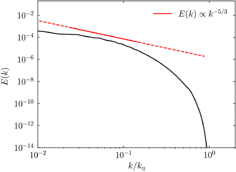
For the present computational experiments, crucial validations have been performed to (i) attain adequate mesh resolution in all three spatial dimensions, and (ii) properly characterize the turbulent flow behavior found in upper-ocean layers. Particularly, to validate the computational accuracy/resolution of the flow model utilized, Fig. 4 depicts the normalized turbulent kinetic energy spectrum E(k) as a function of normalized wavenumber k. As it can be observed from the plot, the energy spectrum reveals two key points: (i) all the important flow scales are sufficiently resolved, as evidenced by the spectrum reaching the Kolmogorov wavenumber kη; and (ii) the classical -5/3 scaling behavior of HIT in the inertial subrange is recovered.
Fig. 4.
Normalized turbulent kinetic energy spectrum E(k) as a function of wavenumber k normalized by Kolmogorov
wavenumber kη. The red line indicates a −5/3 scaling.
4.5. Code availability
The SOLEIL multiphysics flow solver is accessible as open-source [14].
Limitations
The limitation of the current dataset lies in the short simulation times typical of turbulence studies. This may hinder the analysis of the fate of large aggregates over the longer time scales associated with ocean currents, which eventually lead to the formation of marine snow. Another constraint of the short simulation time computed is that particles essentially lack the time to experience the impact of large flow scales and gravity effects, which are therefore excluded from the Lagrangian point particle model and should be considered in future studies. Additionally, the particle model does not consider shape characteristics, such as the impact of fiber or disk microplastics. Nonetheless, as a preliminary open-access data source, the “Distribution and Aggregation of Microparticles in Upper-Ocean Turbulence Dataset” aims to encourage researchers to explore the complex physical behavior of microparticles in the ocean.
Ethics Statement
This work meets ethics requirements and does not involve human subjects, animal experiments, or any data collected from social media platforms and the material is the authors own original work, which has not been previously published elsewhere.
CRediT authorship contribution statement
Federico Pizzi: Conceptualization, Data curation, Formal analysis, Investigation, Writing – original draft. Mona Rahmani: Conceptualization, Investigation, Writing – review & editing. Joan Grau: Conceptualization, Investigation, Writing – review & editing. Francesco Capuano: Conceptualization, Investigation, Funding acquisition, Writing – review & editing. Lluís Jofre: Conceptualization, Investigation, Funding acquisition, Writing – review & editing.
Acknowledgements
This work is funded by the TRITON project (TED2021-132623A-I00) of the Agencia Estatal de Investigación (Spain). The authors gratefully acknowledge the Serra Húnter and SGR (2021-SGR-01045) programs of the Generalitat de Catalunya (Spain), and the computer resources at Cedar provided by the Digital Research Alliance of Canada (RAC-2023 kfw-162-04).
Declaration of Competing Interest
The authors declare that they have no known competing financial interests or personal relationships that could have appeared to influence the work reported in this paper.
Data Availability
References
- 1.Clark J.R., Cole M., Lindeque P.K., Fileman E., Blackford J., Lewis C., Lenton T.M., Galloway T.T.S. Marine microplastic debris: a targeted plan for understanding and quantifying interactions with marine life. Front. Ecol. Environ. 2016;14:317–324. [Google Scholar]
- 2.Eriksen M., Lebreton L.C.M., Carson H.S., Thiel M., Moore C.J., Borerro J.C., Galgani F., Ryan P.G., Reisser J. Plastic pollution in the world's oceans: more than 5 trillion plastic pieces weighing over 250,000 tons afloat at sea. PLOS One. 2014;9 doi: 10.1371/journal.pone.0111913. [DOI] [PMC free article] [PubMed] [Google Scholar]
- 3.Derraik J.G.B. The pollution of the marine environment by plastic debris: a review. Mar. Pollut. Bull. 2002;44:842–852. doi: 10.1016/s0025-326x(02)00220-5. [DOI] [PubMed] [Google Scholar]
- 4.van Sebille E., Wilcox C., Lebreton L., Maximenko N., Hardesty B.D., van Franeker J.A., Eriksen M., Siegel D., Galgani F., Law K.L. A global inventory of small floating plastic debris. Environ. Res. Lett. 2015;10 [Google Scholar]
- 5.Michels J., Stippkugel A., Lenz M., Wirtz K., Engel A. Rapid aggregation of biofilm-covered microplastics with marine biogenic particles. Proc. R. Soc. London, Ser. B. 2018;285 doi: 10.1098/rspb.2018.1203. [DOI] [PMC free article] [PubMed] [Google Scholar]
- 6.Rahmani M., Gupta A., Jofre L. Aggregation of microplastic and biogenic particles in upper-ocean turbulence. Int. J. Multiph. Flow. 2022;157 [Google Scholar]
- 7.F. Pizzi, L. Jofre, F. Capuano, J. Grau, M. Rahmani, Distribution and aggregation of microparticles in upper-ocean turbulence dataset (2024).
- 8.The Figshare Group, Figshare - credit for all your research, 2023.
- 9.Burd A.B., Jackson G.A. Particle aggregation. Annu. Rev. Mar. Sci. 2009;1:65–90. doi: 10.1146/annurev.marine.010908.163904. [DOI] [PubMed] [Google Scholar]
- 10.Daitche A. On the role of the history force for inertial particles in turbulence. J. Fluid Mech. 2015;782:567–593. [Google Scholar]
- 11.Jofre L., Papadakis M., Roy P.T., Aiken A., Iaccarino G. Multifidelity modeling of irradiated particle-laden turbulence subject to uncertainty. Int. J. Uncertain. Quan. 2020;10:499–514. [Google Scholar]
- 12.Jofre L., del Rosario Z.R., Iaccarino G. Data-driven dimensional analysis of heat transfer in irradiated particle-laden turbulent flow. Int. J. Multiph. Flow. 2020;125 [Google Scholar]
- 13.Balachandar S., Eaton J.K. Turbulent dispersed multiphase flow. Annu. Rev. Fluid Mech. 2010;42:111–133. [Google Scholar]
- 14.Stanford. University, Soleil-X: turbulence/particle/radiation solver written in the regent language for execution with the legion runtime, 2014-2019.
- 15.Jofre L., Lehmkuhl O., Ventosa J., Trias F.X., Oliva A. Conservation properties of unstructured finite-volume mesh schemes for the Navier-Stokes equations. Numer. Heat Transfer, Part B. 2014;65:53–79. [Google Scholar]
- 16.Esmaily M., Jofre L., Mani A., Iaccarino G. A scalable geometric multigrid solver for nonsymmetric elliptic systems with application to variable-density flows. J. Comput. Phys. 2018;357:142–158. [Google Scholar]
- 17.Bassenne M., Urzay J., Park G.I., Moin P. Constant-energetics physical-space forcing methods for improved convergence to homogeneous-isotropic turbulence with applications to particle-laden flows. Phys. Fluids. 2016;28 [Google Scholar]
- 18.Thorpe S.A., Osborn T.R., Jackson J.F.E., Hall A.J., Lueck R.G. Measurements of turbulence in the upper-ocean mixing layer using autosub. J. Phys. Oceanogr. 2003;33:122–145. [Google Scholar]
- 19.Eerkes-Medrano D., Thompson R.C., Aldridge D.C. Microplastics in freshwater systems: a review of the merging threats, identification of knowledge gaps and prioritisation of research needs. Water Res. 2015;75:63–82. doi: 10.1016/j.watres.2015.02.012. [DOI] [PubMed] [Google Scholar]
- 20.Stanford University, Exascale computing engineering center. Predictive Science Academic Alliance Program (PSAAP) II, Stanford University, 2014-2019.
Associated Data
This section collects any data citations, data availability statements, or supplementary materials included in this article.


