Geometric diffusions as a tool for harmonic analysis and structure definition of data: Multiscale methods

Abstract

In the companion article, a framework for structural multiscale geometric organization of subsets of and of graphs was introduced. Here, diffusion semigroups are used to generate multiscale analyses in order to organize and represent complex structures. We emphasize the multiscale nature of these problems and build scaling functions of Markov matrices (describing local transitions) that lead to macroscopic descriptions at different scales. The process of iterating or diffusing the Markov matrix is seen as a generalization of some aspects of the Newtonian paradigm, in which local infinitesimal transitions of a system lead to global macroscopic descriptions by integration. This article deals with the construction of fast-order N algorithms for data representation and for homogenization of heterogeneous structures.

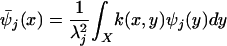
In the companion article (1), it is shown that the eigenfunctions of a diffusion operator, A, can be used to perform global analysis of the set and of functions on a set. Here, we present a construction of a multiresolution analysis of functions on the set related to the diffusion operator A. This allows one to perform a local analysis at different diffusion scales.

This is motivated by the fact that in many situations one is interested not in the data themselves but in functions on the data, and in general these functions exhibit different behaviors at different scales. This is the case in many problems in learning, in analysis on graphs, in dynamical systems, etc. The analysis through the eigenfunctions of Laplacian considered in the companion article (1) are global and are affected by global characteristics of the space. It can be thought of as global Fourier analysis. The multiscale analysis proposed here is in the spirit of wavelet analysis.

We refer the reader to (2–4) for further details and applications of this construction, as well as a discussion of the many relationships between this work and the work of many other researchers in several branches of mathematics and applied mathematics. Here, we would like to at least mention the relationship with fast multiple methods (5, 6), algebraic multigrid (7), and lifting (8, 9).

Multiscale Analysis of Diffusion

Construction of the Multiresolution Analysis. Suppose we are given a self-adjoint diffusion operator A as in ref. 1 acting on ℒ² of a metric measure space (X, d, μ). We interpret A as a dilation operator and use it to define a multiresolution analysis. It is natural to discretize the semigroup {A^t}_t≥0 of the powers of A at a logarithmic scale, for example at the times

[1]

For a fixed ε ∈ (0,1), we define the approximation spaces by

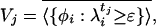[2]

where the φ_is are the eigenvectors of A, ordered by decreasing eigenvalue. We will denote by P_j the orthogonal projection onto V_j. The set of subspaces is a multiresolution analysis in the sense that it satisfies the following properties:

1. lim_j→–∞ V_j = ℒ²(X, μ), .

2. V_j+1 ⊆ V_j for every .

3. is an orthonormal basis for V_j.

We can also define the detail subspaces W_j as the orthogonal complement of V_j in V_j+1, so that we have the familiar relation between approximation and detail subspaces as in the classical wavelet multiresolution constructions:

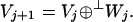This is very much in the spirit of a Littlewood–Paley decomposition induced by the diffusion semigroup (10). However, in each subspace V_j and W_j we have the orthonormal basis of eigenfunctions, but we would like to replace them with localized orthonormal bases of scaling functions as in wavelet theory. Generalized Heisenberg principles (see Extension of Empirical Functions of the Data Set) put a lower bound on how much localization can be achieved at each scale j, depending on the spectrum of the operator A and on the space on which it acts. We would like to have basis elements as much localized as allowed by the Heisenberg principle at each scale, and spanning (approximately) V_j. We do all this while avoiding computation of the eigenfunctions.

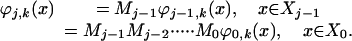
We start by fixing a precision ε > 0 and assume that A is represented on the basis Φ₀ = {δ_k}_kεX. We consider the columns of A, which can be interpreted as the set of functions on X. We use a local multiscale Gram–Schmidt procedure, described below, to carefully but efficiently orthonormalize these columns into a basis Φ₁ = {ϕ_1,k}_kεX1 (X₁ is defined as this index set) for the range of A up to precision ε. This is a linear transformation we represent by a matrix G₀. This yields a subspace that is ε-close to V₁. Essentially, Φ₁ is a basis for a subspace that is ε-close to the range of A, the basis elements that are well localized and orthogonal. Obviously, |X₁| ≤ |X|, but the inequality may already be strict since part of the range of A may be below the precision ε. Whether this is the case or not, we have then a map M₀ from X to X₁, which is the composition of A with the orthonormalization by G₀. We can also represent A in the basis Φ₁: We denote this matrix by A₁ and compute . See the diagram in Fig. 1.

Fig. 1.

Diagram for downsampling, orthogonalization, and operator compression.

We now proceed by looking at the columns of , which are up to precision ε, by unraveling the bases on which the various elements are represented. Again we can apply a local Gram–Schmidt procedure to orthonormalize this set: This yields a matrix G₁ and an orthonormal basis Φ₂ = {ϕ_2,k}_kεX2 for the range of up to precision ε, and hence for the range of up to precision 2ε. Moreover, depending on the decay of the spectrum of A, |X₂| << |X₁|. The matrix M₁, which is the composition of G₁ with , is then of size |X₂| × |X₁|, and is a representation of A⁴ acting on Φ₂.

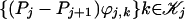
After j steps in this fashion, we will have a representation of A^{1+2+22+· · ·+2j} = A^2j+1–1 onto a basis Φ_j = {ϕ_j,k}_kεXj that spans a subspace which is jε-close to V_j. Depending on the decay of the spectrum of A, we expect |X_j| << |X|; in fact, in the ideal situation§ the spectrum of A decays fast enough so that there exists γ < 1 such that |X_j| < γ^2j+1–1|X|. This subspace is spanned by “bump” functions at scale j, as defined by the corresponding power of the diffusion operator A. The “centers” of these bump functions can be identified with X_j, which we can think of X_j as a coarser version of X. The basis Φ_j is naturally identified with the set of Dirac δ-functions on X_j; however, one can extend these functions, defined on the “compressed” graph X_j, to the whole initial graph X by writing

[3]

Since every function in Φ₀ is defined on X, so is every function in Φ_j. Hence, any function on the compressed space X_j can be extended naturally to the whole X. In particular, one can compute low-frequency eigenfunctions on X_j and then extend them to the whole X. This is of course completely analogous to the standard construction of scaling functions in the Euclidean setting (5, 11, 12). Observe that each point in X_j can be considered as a “local aggregation” of points in X_j–1, which is completely dictated by the action of the operator A on functions on X: A itself is dictating the geometry with respect to which it should be analyzed, compressed, and applied to any vector.

We have thus computed and efficiently represented the powers A^2j, for j > 0, that describe the behavior of the diffusion at different time scales. This applies to the solution of discretized of partial differential equations, of Markov chains, and in learning and related classification problems.

Wavelet Transforms and Green's Function. The construction immediately suggests an associated fast scaling function transform: Suppose we are given f on X and want to compute 〈f, ϕ_j,k〉 for all scales j and corresponding “translations” k. Being given f is equivalent to saying we are given (〈f, ϕ_0,k〉)_kεX. Then we can compute (〈f, ϕ_1,k〉)_kεX1 = M₀ (〈f, ϕ_0,k〉)_kεX, and so on for all scales. The matrices M_j are sparse (since A_j and G_j are), so this computation is fast. This generalizes the classical scaling function transform. We will see later that wavelets can be constructed as well and a fast wavelet transform is possible.

In the same way, any power of A can be applied fast to a function f. In particular, Green's function (I – A)^–1 can be applied fast to any function. Since

if we let 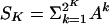, we see that

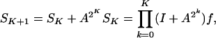and each term of the product can be applied fast to f.

The construction of the multiscale bases can be done in time Ο(n log² n), where n = |X|, if the spectrum of A has fast enough decay. The decomposition of a function f onto the scaling functions and wavelets we construct can be done in the same time, and so does the computation of (I – A)^–1 f.

The Orthogonalization Process. We sketch here how the orthogonalization works (for details, refer to refs. 2 and 3). Suppose we start from a δ-local basis (in our case, ϕ_x is going to be a bump A^lδ_x). We greedily build a first layer of basis functions 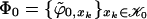, as follows. We let ϕ_0,x0 be a basis function with greatest ℒ²-norm. Then we let ϕ_0,x1 be a basis function with biggest ℒ²-norm among the basis functions with support disjoint from the support of ϕ_0,x0 but not farther than δ from it. By induction, after ϕ_0,x0,..., ϕ_0,xl have been chosen, we let ϕ_0,xl+1 be a scaling function with largest ℒ²-norm among those having a support that does not intersect any of the supports of the basis functions already constructed but is not farther than δ from the closest such support. We stop when no such choice can be made. One can think of roughly as a 2δ lattice.

At this point, Φ₀ in general spans a subspace much smaller than the one spanned by Φ. We construct a second layer , as follows. Orthogonalize each to the functions 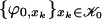. Observe that since the support of ϕ_x is small, this orthogonalization is local, in the sense that each ϕ_x needs to be orthogonalized only to the few that have an intersecting support. In this way, we get a set , orthogonal to Φ₀ but not orthogonal itself. We orthonormalize it exactly as we did to get Φ₀ from Φ. We proceed by building as many layers as necessary to span the whole space 〈Φ〉 (up to the specified precision ε).

Wavelets. We would like to construct bases {ψ_j,k}_k for the spaces W_j, j ≥ 1, such that V_j ⊕^⊥ W_j = V_j+1. To achieve this, after having built and 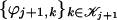, we can apply our modified Gram–Schmidt procedure with geometric pivoting to the set of functions

which will yield an orthonormal basis of wavelets for the orthogonal complement of V_j+1 in V_j. Observe that each wavelet is a result of an orthogonalization process that is local, so the computation is again fast. To achieve numerical stability, we orthogonalize at each step the remaining ϕ_j+1,ks to both the wavelets built so far and ϕ_j,k. Wavelet subspaces can be recursively split further to obtain diffusion wavelet packets (4), which allow the application of the classical fast algorithms (13) for denoising (14), compression (15), and discrimination (16).

Examples and Applications

Example 3.1: Multiresolution diffusion on the homogeneous circle. To compare with classical constructions of wavelets, we consider the unit circle, sampled at 256 points, and the classical isotropic heat diffusion on it. The initial orthonormal basis Φ₀ is given by the set of δ-functions at each point, and we build the diffusion wavelets at all scales, which clearly relate to splines and multiwavelets. The spectrum of the diffusion operator does not decay very fast (see Figs. 2 and 3).

Fig. 2.

Diffusion multiresolution analysis on the circle. We consider 256 points on the unit circle, starting with ϕ_0,k = δ_k and with the standard diffusion. We plot several scaling functions in each approximation space V_j.

Fig. 3.

Diffusion multiresolution analysis on the circle. We plot the compressed matrices representing powers of the diffusion operator, in white are the entries above working precision (here set to 10^–8). Notice the shrinking of the size of the matrices which are being compressed at the different scales.

Example 3.2: Dumbbell. We consider a dumbbell-shaped manifold, sampled at 1,400 points, and the diffusion associated to the (discretized) Laplace–Beltrami operator as discussed in ref. 1. See Fig. 4 for the plots of some scaling functions and wavelets: They exhibit the expected locality and multiscale features, dependent on the intrinsic geometry of the manifold.

Fig. 4.

Some diffusion scaling functions and wavelets at different scales on a dumbbell-shaped manifold sampled at 1,400 points.

Example 3.3: Multiresolution diffusion on a nonhomogeneous circle. We can apply the construction of diffusion wavelets to nonisotropic diffusions arising from partial differential equations, to tackle problems of homogenization in a natural way. The literature on homogenization is vast (see, e.g., refs. 17–21 and references therein).

Our definition of scales, driven by the differential operator, in general results in highly nonuniform and nonhomogeneous spatial and spectral scales, and in corresponding coarse equations of the system, which have high precision.

For example, we can consider the nonhomogeneous heat equation on the circle

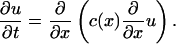[4]

where c(x) is a positive function close 0 at certain points and almost 1 at others. We want to represent the intermediate and large scale/time behavior of the solution by compressing powers of the operator representing the discretization of the spatial differential operator ∂/∂x(c(x)(∂/∂x)). The spatial differential operator on the right-hand side of Eq. 4 is a matrix T that, when properly normalized, can be interpreted as a nontranslation invariant random walk. Our construction yields a multiresolution associated to this operator that is highly nonuniform, with most scaling functions concentrated around the points where the conductivity is highest, for several scales. The compressed matrices representing the (dyadic) powers of this operator can be viewed as multiscale homogenized versions, at a certain scale that is time and space dependent, of the original operator (see Fig. 5).

Fig. 5.

Multiresolution diffusion on a circular medium with non-constant diffusion coefficient. (Upper) Several scaling functions and wavelets in different approximation subspaces V_j. Notice that scaling functions at the same diffusion scale exhibit different spatial localization, which depends on the local diffusion coefficient. (Lower) Matrix compression of the dyadic powers of T on the scaling function bases of the V_js. Notice the size of the matrices shrinking with scale.

While the examples above illustrate classical settings, the construction of diffusion wavelets carries over unchanged to weighted graphs, by considering the generator of the diffusion associated to the natural random walk (and Laplacian) on the graph. It then allows a natural multiscale analysis of functions of interest on such a graph. We expect this to have a wide range of applications to the analysis of large data sets, document corpora, network traffic, etc., which are naturally modeled by graphs.

Extension of Empirical Functions of the Data Set

An important aspect of the multiscale developed so far involves the relation of the spectral theory on the set to the localization on and off the set of the corresponding eigenfunctions and diffusion scaling functions and wavelets. In addition to the theoretical interest of this topic, the extension of functions defined on a set X to a larger set X̄ is of critical importance in applications such as statistical learning. To this end, we construct a set of functions, termed geometric harmonics, that allow one to extend a function f off the set X, and we explain how this provides a multiscale analysis of f. For a more detailed studied of geometric harmonics, the reader is referred to ref. 22.

Construction of the Extension: The Geometric Harmonics. Let us specify the mathematical setting. Let X be a set contained in a larger set X̄, and μ be a measure on X. Suppose that one is given a positive semidefinite symmetric kernel k(·, ·) defined on X̄ × X̄, and if f is defined on X, let K: L²(X, μ) → L² (X, μ) be defined by

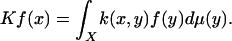Let {ψ_j} and be the eigenfunctions and eigenvalues of this operator. Note that under weak hypotheses, the operator K is compact, and its eigenfunctions form a basis of L²(X, μ). Then, by definition, if , then

where this identity holds for x ε X. Now, if we let x be in X̄, the right-hand side of this equation is well defined, and this allows one to extend ψ_j as a function defined on X̄. This procedure, which goes by the name of Nyström extension, has already been suggested to overcome the problem of large-scale data sets (23) and to speed up the data processing (24).

From the above, each extension is constructed as an integral of the values over the smaller set X and consequently verifies some sort of mean value theorem. We call these functions geometric harmonics.

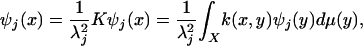
From the numerical analysis point of view, one has to be careful as λ_j → 0 as j → +∞, and one can extend only the eigenfunctions ψ_j for which , where δ > 0 is preset number. We can now safely define the extension of function f from X to X̄ by

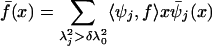for x ∈ X̄, where 〈·, ·〉_X is the inner product of L²(X, μ). This way, the extension operation has condition number 1/δ. We immediately notice that for f̄ to approximately coincide with f on X, one must have that most of the energy of f be concentrated in the first few eigenfunctions ψ_j.

Let us give three examples of geometric harmonics. The first example is related to potential theory. Assume that X is a smooth closed hypersurface of , dμ = dx and consider the Newtonian potential in :

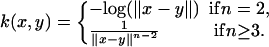Then the geometric harmonics have the form

and are obviously harmonic in the domain with boundary X. If f is a function on X representing the single layer density of charges on X, then the extension f̄ is, by construction, a sum of harmonic functions and an harmonic extension of f.

For the second example, consider a Hilbert basis of a subspace . For instance, this could be a wavelet basis of some finite-scale shift-invariant space. Then the diagonalization of the restriction of kernel

to a set X generates geometric harmonics, and an extension procedure of empirical functions on X to functions of V.

The third example is of particular importance because it generalizes the prolate spheroidal wave functions introduced in the context of signal processing in refs. 25 and 26. Assume that and consider the space V_B of bandlimited functions with fixed band B > 0 (we call these functions B-bandlimited). Following the procedure explained in the second example, we can construct geometric harmonics that are B-bandlimited. It can be shown that this comes down to diagonalizing the kernel

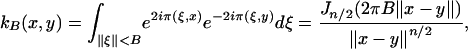where x and y belong to X, and J_ν is the Bessel function of the first type and of order ν. From the first equality sign, we see that the geometric harmonics arise from a principal component analysis of the set of all restrictions of B-bandlimited complex exponentials to X.

It can verified that, in addition to be orthogonal on the set X, these B-bandlimited geometric harmonics are also orthogonal over the whole space . Moreover, minimizes the Rayleigh quotient

under the constraint that f be orthogonal to {ψ₀, ψ₁,..., ψ_j–1}. In other words, is the B-bandlimited extension of ψ_j that has minimal energy on . As a consequence, f̄ is the B-bandlimited extension of f that has minimal energy off the set X. This type of extension is optimal in the sense that it is the average of all B-bandlimited extension of f. It also suggests that this extension satisfies Occam's razor in that it is the “simplest” among all bandlimited extensions: Any other extension is equal to f̄ plus an orthogonal bandlimited function that vanishes on X.

Multiscale Extension. For a given function f on X, we have constructed a minimal energy B-bandlimited extension f̄. In the case when X is a smooth compact submanifold of , we can now relate the spectral theory on the set X to that on .

On the one hand, any band limited function of band B > 0 restricted to X can be expanded to exponential accuracy in terms of the eigenfunctions of the Laplace–Beltrami operator Δ with eigenvalues not exceeding CB² for some small constant C > 0. On the other hand, it can be shown that every eigenfunction of the Laplace–Beltrami operator satisfying this condition extends as a bandlimited function with band C′B. Both of these statements can be proved by observing that eigenfunctions on the manifold are well approximated by restrictions of bandlimited functions.

We conclude that any empirical function f on X that can be approximated as a linear combination of eigenfunctions of Δ, and these eigenfunctions can be extended to different distances: If the eigenvalue is ν², then the corresponding eigenfunction can be extended as a ν-bandlimited function off the set X to a distance Cν^–1. This observation constitutes a formulation of the Heisenberg principle involving the Fourier analysis on and off the set X, and which states that any empirical function can be extended as a sum of “atoms” whose numerical supports in the ambient space is related to their frequency content on the set.

The generalized Heisenberg principle is illustrated on Fig. 6, where we show the extension of the functions f_j(θ) = cos(2πjθ)for j = 1, 2, 3 and 4, from the unit circle to the plane. For each function, we used Gaussian kernels, and the scale was adjusted as the maximum scale that would preserve a given accuracy.

Fig. 6.

Extension of the functions f_j(θ) = cos(2πjθ) for j = 1, 2, 3, and 4, from the unit circle to the plane.

Conclusion

We have introduced a multiscale structure for the efficient computation of large powers of a diffusion operator, and its Green function, based on a generalization of wavelets to the general setting of discretized manifolds and graphs. This has application to the numerical solution of partial differential equations and to the analysis of functions on large data sets and learning. We have shown that a global (with eigenfunctions of the Laplacian) or local (with diffusion wavelets) analysis on a manifold embedded in Euclidean space can be extended outside the manifold in a multiscale fashion by using band-limited functions.

References

- 1.Coifman, R. R., Lafon, S., Lee, A. B., Maggioni, M., Nadler, B., Warner, F. & Zucker, S. W. (2005) Proc. Natl. Acad. Sci. USA 102, 7426–7431. [DOI] [PMC free article] [PubMed] [Google Scholar]
- 2.Coifman, R. R. & Maggioni, M. (2004) Tech. Rep. YALE/DCS/TR-1289 (Dept. Comput. Sci., Yale Univ., New Haven, CT).
- 3.Coifman, R. R. & Maggioni, M. (2004) Tech. Rep. YALE/DCS/TR-1303, Yale Univ. and Appl. Comput. Harmonic Anal., in press.
- 4.Bremer, J. C., Jr., Coifman, R. R., Maggioni, M. & Szlam, A. D. (2004) Tech. Rep. YALE/DCS/TR-1304, Yale Univ. and Appl. Comput. Harmonic Anal., in press.
- 5.Beylkin, G., Coifman, R. R. & Rokhlin, V. (1991) Comm. Pure Appl. Math 44, 141–183. [Google Scholar]
- 6.Greengard, L. & Rokhlin, V. (1987) J. Comput. Phys. 73, 325–348. [Google Scholar]
- 7.Brandt, A. (1986) Appl. Math. Comp. 19, 23–56. [Google Scholar]
- 8.Sweldens, W. (1996) Appl. Comput. Harmonic Anal. 3, 186–200. [Google Scholar]
- 9.Sweldens, W. (1997) SIAM J. Math. Anal. 29, 511–546. [Google Scholar]
- 10.Stein, E. (1970) Topics in Harmonic Analysis Related to the Littlewood–Paley Theory (Princeton Univ. Press, Princeton), Vol. 63.
- 11.Meyer, Y. (1990) Ondelettes et Operatéurs (Hermann, Paris).
- 12.Daubechies, I. (1992) Ten Lectures on Wavelets (Soc. for Industrial and Appl. Math., Philadelphia).
- 13.Coifman, R. R., Meyer, Y., Quake, S. & Wickerhauser, M. V. (1993) in Progress in Wavelet Analysis and Applications (Toulouse, 1992) (Frontières, Gif-Sur-Yvette, France), pp. 77–93.
- 14.Donoho, D. L. & Johnstone, I. M. (1994) Ideal Denoising in an Orthonormal Basis Chosen from a Library of Bases (Stanford Univ., Stanford, CA).
- 15.Coifman, R. R. & Wickerhauser, M. V. (1992) IEEE Trans. Info. Theory 38, 713–718. [Google Scholar]
- 16.Coifman, R. R. & Saito, N. (1994) C. R. Acad. Sci. 319, 191–196. [Google Scholar]
- 17.Babuska, I. (1976) Numerical Solutions of Partial Differential Equations (Academic, New York), Vol. 3, pp. 89–116. [Google Scholar]
- 18.Gilbert, A. C. (1998) Appl. Comp. Harmonic Anal. 5, 1–35. [Google Scholar]
- 19.Beylkin, G. & Coult, N. (1998) Appl. Comp. Harmonic Anal. 5, 129–155. [Google Scholar]
- 20.Hackbusch, W. (1985) Multigrid Methods and Applications (Springer, New York).
- 21.Knapek, S. (1998) SIAM J. Sci. Comput. 20, 515–533. [Google Scholar]
- 22.Coifman, R. R. & Lafon, S. (2004) Appl. Comp. Harmonic Anal., in press.
- 23.Fowlkes, C., Belongie, S., Chung, F. & Malik, J. (2004) IEEE Pattern Anal. Machine Intell. 26, 214–225. [DOI] [PubMed] [Google Scholar]
- 24.Williams, C. & Seeger, M. (2001) in Advances in Neural Information Processing Systems 13: Proceedings of the 2000 Conference, eds. Leen, T. K., Dietterich, T. G. & Tresp, V. (MIT Press, Cambridge, MA), pp. 682–688.
- 25.Slepian, D. & Pollack, H. O. (1961) Bell Syst. Tech. J. 40, 43–64. [Google Scholar]
- 26.Slepian, D. (1964) Bell Syst. Tech. J. 43, 3009–3058. [Google Scholar]