Hamilton's indicators of the force of selection

Abstract

To quantify the force of selection, Hamilton [Hamilton, W. D. (1966) J. Theor. Biol. 12, 12–45] derived expressions for the change in fitness with respect to age-specific mutations. Hamilton's indicators are decreasing functions of age. He concluded that senescence is inevitable: survival and fertility decline with age. I show that alternative parameterizations of mutational effects lead to indicators that can increase with age. I then consider the case of deleterious mutations with age-specific effects. In this case, it is the balance between mutation and selection pressure that determines the equilibrium number of mutations in a population. In this balance, the effects of different parameterizations cancel out, but only to a linear approximation. I show that mutation accumulation has little impact at ages when this linear approximation holds. When mutation accumulation matters, nonlinear effects become important, and the parameterizations of mutational effects make a difference. The results also suggest that mutation accumulation may be relatively unimportant over most of the reproductive lifespan of any species.

Senescence can be defined as an increase in mortality and/or a decrease in fertility with age. Is senescence a universal characteristic of life? It is not obvious from an evolutionary perspective why it should be. Early in life, when individuals develop and grow, mortality falls and reproductive potential increases. Why is it that these age patterns cannot persist, in some form, with mortality continuing to decline and reproductive capacity continuing to increase?

William D. Hamilton's influential article on “The Moulding of Senescence by Natural Selection” (1, 2) provides one reason why senescence “cannot be avoided by any conceivable organism.” Hamilton combines insights about the evolution of senescence (3, 4) with concepts and models of population dynamics (5). Hamilton asserts that “senescence is an inevitable outcome of evolution.” His results imply that mortality rises and fertility falls from reproductive maturity onwards. Did Hamilton genuinely prove that senescence is universal?

Hamilton's Derivations

How does a mutation that acts only at a specific age a influence the evolutionary success of an individual? Does it matter if this age is early or late in life? Hamilton (1) built on the insight of Medawar (3) that later-acting genes should be under weaker selection than earlier-acting ones due to the unavoidable decline in the number of survivors at higher and higher ages. A genetically determined fatal disease that struck only at post-reproductive ages would be entirely out of reach of the force of selection.

The Framework. To quantify the force of selection, Hamilton considered age-specific mutation-induced changes in fitness. Hamilton used the most widely accepted measure of Darwinian fitness, the intrinsic rate of population increase r, implicitly defined by the discrete version of the Lotka equation,

[1]

The function l_x gives the chance of survival to age x. The function m_x measures the amount of reproduction at that age. If the population is stable, as assumed by Hamilton, then each combination of an age-specific maternity function m_x and an age-specific survival function l_x is associated with exactly one real r that satisfies Eq. 1. The survival function l_x is defined as the product of the probabilities p_a of survival from age a to a + 1:

[2]

with

The age-specific survival probabilities p_a depend on the instantaneous death rate μ_t, the force of mortality between age a and a + 1, via

[3]

The cumulated mortality in the exponent reflects the average mortality during that time interval, denoted by .

Hamilton's Survival Indicator. By taking the derivative of Eq. 1 with respect to ln p_a and rearranging, Hamilton derived his basic result:

[4a]

Note that Eq. 3 implies that H^† can also be expressed as:

[4b]

The value of H^† is a measure of the force of selection. It captures the change in fitness r induced by an increase in ln p_a. An increase in ln p_a is equivalent to a reduction in average mortality between age a and a + 1. This sensitivity of fitness to changes in age-specific survival is captured by the ratio of remaining reproduction, the numerator of Eq. 4a, to generation time, the denominator. Because H^† declines as age increases, Hamilton concluded that the force of selection must decline with age.

Alternative Indicators

Different Parameterizations. Hamilton's conclusion hinges on the particular parameterization he chose for the nature of the effect of a mutation. Equally reasonable, alternative forms would have been dr/dp_a, dr/dq_a, dr/d ln q_a, or dr/d ln , where q_a is the probability of dying, and , as noted above, equals -ln p_a. The results are as follows:

[5a]

[5b]

[5c]

and

[5d]

Strikingly, the expressions in Eq. 5a, 5b, 5c, 5d can increase in absolute value with age in contrast to H^†, which always declines.

When Selection Pressure Increases. Consider, for instance, Eq. 5d. At prereproductive ages, the value of dr/d ln is entirely determined by , because H^† is constant before maturity. At reproductive ages, the change in fitness with respect to mortality increases from age a to a + 1 if

Substituting Eqs. 5d and 4a and using the notion of reproductive value, introduced by Fisher (6),

[6]

this inequality can be rearranged to give the following condition,

[7]

Hence, the value of dr/d ln will increase with age if < and if future reproductive value is sufficiently large compared to fertility m_a+1. Taking into account the fact that Eq. 1 must hold, the inequality in Eq. 7 can be rearranged as

[8]

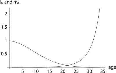
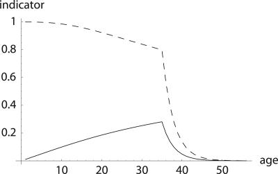
This inequality determines trajectories for m_a+1 that lead to increasing sensitivity of fitness to changes in mortality over age given a specified increasing path for . The survival and fertility functions plotted in Fig. 1 and the resulting indicators dr/d ln and dr/d ln p_a plotted in Fig. 2 provide an illustrative example.

Fig. 1.

Example of survival and maternity functions l_a and m_a. If age-specific survival probabilities p_a change according to with p₀ < 1, then the average force of mortality between age a and a + 1 is given by . Maternity m_a+1 was chosen to be 0.01 units smaller than the left-hand side of the inequality in Eq. 8, setting r = 0, p₀ = 0.99 and m₀ = 0. By age 34, survival falls to 0.25%. After age 34, I fixed age-specific survival p_a at its level of p₃₅ = 0.70 corresponding to and adjusted m_a to a constant level of 133.265 such that Eq. 1 is fulfilled.

Fig. 2.

Comparison of H^† = dr/d ln p_a (dashed line) with dr/d ln (solid line). While Hamilton's indicator H^† declines, the alternative one increases until age 34. The increase would have continued if m_a+1 was further determined by the inequality in Eq. 8. This, however, would result in a trajectory for m_a that would rise to enormous heights. Also note that Hamilton's indicator is greater than the alternative indicator, especially before age 35. This implies a considerably stronger force of selection on age-specific mutations that affect mortality.

Fertility Indicators. The quantity Hamilton derived for the force of selection on age-specific mutations that affect fertility is

[9]

Hamilton considered survival effects on a log scale. He could have done the same for reproduction, calculating

[10]

Hamilton's indicator in Eq. 9 necessarily declines with age, but the alternative indicator in Eq. 10 can increase with age depending on the trajectory of m_a.

Table 1 summarizes the direction of changes over age of the various indicators of the force of selection. The differences in the dynamics are due to the nonlinearity of logarithmic transformations.

Table 1. Various indicators of the force of selection in Hamilton's framework.

Indicator	Change with age a
	—
	+ or -
	+ or -
	+ or -
	+ or -
	—
	+ or -

+ or–means that the change with age can be positive or negative depending on the trajectories of m_x and I_x.

Are Some Indicators Better? Charlesworth (ref. 7, p. 191), who reconstructed Hamilton's results, suggested that “genetic effects on survival probabilities are more likely to be additive on a log scale.” His conjecture implies that mutations have additive effects on mortality. Indeed, both of Hamilton's indicators H^† = and H^* = dr/dm can be interpreted as assuming that mutations additively affect average mortality and fertility m. This is plausible, because additive risk models are widely used, most commonly in evolutionary modeling (8, 9). The indicators and mH^* capture the effect of a proportional change in and m. Proportional-hazard models in general, and Cox proportional-hazard models (10) in particular, are frequently used in demographic and epidemiological research.

Whether age-specific mutations act proportionally or additively is an open question for empirical research. Numerous demographic and epidemiological analyses of risk factors have found that proportional effects are more common than additive effects. In particular, the impact of genetic polymorphisms, such as ApoE 2, 3, and 4, on mortality has been modeled by proportional hazards (11). Empirical results of Promislow and Tatar (12) support the proportional-hazard assumption, suggesting that mutations act additively on log-mortality rather than log-survival. Hence, it seems plausible that the indicators and mH^* will prove at least as valid as Hamilton's indicators.

Optimization vs. Mutational Burden. How mutations affect fitness is the focus of a vast literature (7, 13–18). Since Medawar (3) and Hamilton (1), many biologists have considered the sensitivity of fitness with respect to age-specific changes in survival or fertility (9) as an indicator of selection pressure. A key issue is whether age patterns of mortality and fertility are moulded by adaptive optimization processes or the burden of nonadaptive mutations (7, 19). Optimization models can be solved without using Hamilton's indicators (20). If the age patterns mainly reflect the age-specific burden of mutations, then Hamilton's indicators are not sufficient. Age-specific levels of birth and death rates depend not only on selection pressure but also on mutation rates. In the following section, I analyze this balance.

Mutation-Selection Balance

How do the different parameterizations in Table 1 affect the equilibrium number of deleterious mutations at each age? In particular, is the magnitude of mutation accumulation great enough to mould the trajectory of mortality?

The equilibrium number of mutations under mutation-selection balance can be approximated by the ratio of the total mutation rate ν (i.e., the hazard of a mutation from a set of possible mutations) and the change in fitness r:

[11]

where n denotes the number of mutations, and n̄ denotes the equilibrium number (ref. 7, pp. 125 and 126). The approximation holds if n̄ is small. Using the chain rule, the derivative in Eq. 11 can be factored into the change in fitness with respect to survival or fertility and the effect on survival or fertility of having n mutations:

[12]

where f could be any of the denominators in Table 1.

Additive vs. Proportional Parameterization. Consider a mutation that has a small effect δ on mortality. Then f equals:

[13a]

in the additive case and

[13b]

in the proportional case. From Eqs. 11 and 12 and Table 1, it follows that

[14a]

in the additive case and

[14b]

in the proportional case. In these ratios, h^†_a denotes remaining reproduction at age a of an individual with no deleterious mutations. It is related to Hamilton's indicator via h^†_a = H^†_aT, where T captures generation time.

Combining Eqs. 13 and 14 leads to the result

[15a]

in the additive case and

[15b]

in the proportional case. If mutations are rare, then

[16]

Hence, if ν and n̄ are small enough that the approximations in Eqs. 11 and 16 hold, then mutation accumulation will result in about the same age-specific mortality regardless of whether mutations have additive or proportional effects.

A Simple Box Model. If n̄ is large, an alternative approach is necessary. Several helpful models have been developed (e.g., refs. 21–24); for a review, see Bürger (18) and Charlesworth (7). A recent general model by Steinsaltz, Evans, and Wachter (25) includes earlier models as special cases.

A solution based on a simple box model, similar to that of Kimura and Maruyama (21), can be readily developed. Assume a haploid asexual population that is stationary. Further assume that mutations affect only one age class, to ensure that the equilibrium numbers of mutations are independent across ages. Focus on a single age a. Individuals are sorted into boxes according to their number of mutations at age a. Let N(n) be the number of individuals in box n, and let N be the total constant population size at age a. In mutation-selection balance, the proportions N(n)/N are fixed. Denote an individual's lifetime reproduction in box n by R(n). Let ν be the probability of passing on a mutation to the next generation. Assume that mutations occur successively, i.e., it is not possible to jump over boxes. Ignore back mutations. Mutations are deleterious, therefore R(0) > R(1) > R(2)... > R(K), K being some maximum number.

The number of individuals N(n) in box n is given by the inflow of individuals minus the outflow per generation,

[17]

It follows immediately that reproduction in box zero is

[18]

In the case of mutations that affect mortality, the lifetime reproduction of individuals in the nth box is given by

[19]

This result can be expressed as

[20]

where Δ(n) is the fraction of remaining reproduction h^†_a that is lost due to carrying n mutations. In the additive case,

[21a]

and in the proportional case,

[21b]

It follows from Eqs. 17 and 20 that

[22]

The equilibrium number of mutations is the average over all boxes, i.e.,

[23]

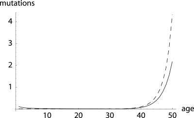
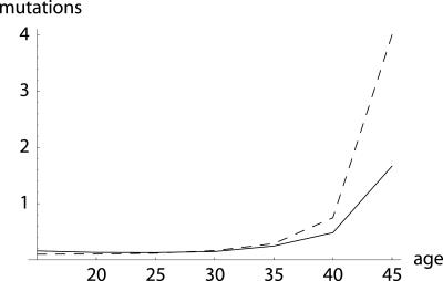
Fig. 3 plots the equilibrium number of mutations over age in the additive versus proportional case for the example presented in Figs. 1 and 2. As a second example, I consider female mortality, as given in the Swedish life table for 1778–1782. Results are shown in Figs. 4 and 5.

Fig. 3.

Equilibrium number of mutations: additive (dashed line) and proportional (solid line). I assume that mutation pressure ν = 0.001. Furthermore, I assume that a mutation at any age reduces remaining reproduction by ≈10% in both the additive and proportional cases. This refers to an average reduction in the proportional case, because Δ(n) depends on the level of mortality at age a, as can be seen from Eq. 21b. Specifically, δ = 0.1 in Eq. 21a and δ = 0.35 in Eq. 21b. Although in the Hamiltonian case of an additive hazard, the number of mutations remains low and then increases with age, proportional effects lead to an age-specific mutational load that declines at young ages. In the example, only one-quarter of 1% of individuals are alive at age 34. Before this age, the mutational load is close to zero. After this age, however, the equilibrium number of mutations sharply rises.

Fig. 4.

Equilibrium number of mutations: additive (dashed line) and proportional (solid line). The example is based on female mortality, as given in the Swedish life table for 1778–1782, for seven 5-year age groups, beginning at age 15. Because the Swedish population was growing at that time, I normalized reproduction to ensure R = 1.00. I consider a deleterious mutation that reduces remaining reproduction at any age by ≈1%, either in an additive or in a proportional way, i.e., δ = 0.01 in Eq. 21a and δ = 0.7 in Eq. 21b, and I assume a mutation pressure of ν = 0.001. The difference between the additive and proportional case increases at higher ages, as levels of remaining reproduction decline. A slight decrease in the equilibrium number of mutations from the first to the second age group can be observed.

Fig. 5.

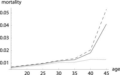
Mortality: additive (dashed line), proportional (solid line), and initial mortality μ_a(0) (dotted line). Initial mortality is from the Swedish life table for 1778–1782, females, for seven 5-year age groups, beginning at age 15.

The values of h^† that determine the numbers of mutations in Figs. 3 and 4 are calculated by using specific initial fertility and mortality schedules. The mutations, however, will raise mortality, producing a new schedule that determines a new h^†. These dynamics are beyond the scope of this article. Note, however, that higher hazard rates would reduce the fitness costs of a change in age-specific mortality. Therefore, more mutations would accumulate, and the difference between additive and proportional parameterizations would be larger than predicted by my conservative estimate. A general treatment that takes into account interactions between ages is given by Steinsaltz, Evans, and Wachter (25).

The Importance of Mutation Accumulation

The age-trajectory of mortality can be decomposed into three parts: one fraction is due to the accumulation of unfavorable mutations, another fraction results from selection processes that optimize the trade-offs necessitated by resource limitations, and the remaining fraction can be attributed to unavoidable external risks of death. How strong is the influence of mutation accumulation?

The relative impact of mutation accumulation on the moulding of the mortality trajectory is crucially determined by the ratio of mutation pressure ν to remaining reproduction h^†_a, as indicated by Eq. 14. The larger ν is, the more influential is mutation accumulation. But what is the magnitude of ν? Kimura and Maruyama (21) and Drake et al. (26) suggest mutation rates per genome per generation of ≈0.1 and between 0.1 and 100, respectively. More recent publications estimate the genomic rate of deleterious mutations in humans to be at least 1.6 (27) or even 3 (28) per generation. If the fraction of mutations that exclusively affect mortality at a specific age is low, then these values could be consistent with a value of ν = 0.001. If ν is 0.001, then Fig. 6 suggests that the influence of mutation accumulation is likely to be small over the major part of reproductive life. This is speculation, however, until the magnitude of ν is estimated empirically.

Fig. 6.

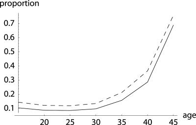
Proportion of mortality explained by mutation accumulation: additive (dashed line) vs. the proportional (solid line) case. The fraction 1 - μ_a(0)/μ_a(n̄) indicates the proportion of equilibrium mortality that can be explained by the accumulation of mutations. For the example of Swedish females, when ν = 0.001, over the main span of reproductive life mutation accumulation explains less than one-third of total mortality. Note, however, that at ages 45–50, when mortality is high, mutation accumulation accounts for the bulk of total mortality.

The conclusions drawn above and in the previous section were reached on the basis of a specific model of mutation accumulation. In general cases covered by the solutions given by Steinsaltz, Evans, and Wachter (25), the form of the mutation-selection equilibrium depends on the extent of assumed genetic recombination. At both extremes, in the absence of recombination (equation 9 in ref. 25) and in the presence of free recombination (equation 27 in ref. 25), the parameterization of the mutational effect, i.e., whether the effect is additive or proportional, influences the mutation-selection equilibrium.

Discussion

Human mortality rises much more slowly than suggested by the results in Fig. 6. This leads to a problem not yet touched on. All the indicators in Table 1 imply that the force of selection drops to zero when reproduction ceases. Several authors (29–32) have argued that lethal mutations could accumulate, yielding a black hole of death at the age when reproduction ends. This could have been shown in Figs. 3, 4, 5 if the curves where drawn to higher ages. As h^†_a approaches ν, the equilibrium number of mutations steeply rises.

Various species, however, enjoy an extended period of post-reproductive life, at least under protected conditions. High external mortality in the wild generally ensures that few individuals survive to old age. Therefore, a rapid increase in mortality should be observed in captivity or in the laboratory at ages when remaining reproduction in the wild is low. Mortality trajectories at older ages, however, have been found to level off and, in some studies, to decline for humans and various species kept in protected environments (33). These findings appear to be inconsistent with mutation accumulation theory. Models of mutation accumulation need to be combined with trade-off models of the evolution of senescence to clarify the dynamics of demographic schedules (20, 34).

In a stimulating but problematic article, Lee (35) conjectures that it is the age pattern of resource transfer rather than of fertility that determines the age pattern of mortality for humans and perhaps other species. Intergenerational transfers that are made before, at, and after birth could significantly influence the evolution of life-history schedules for a wide variety of species. In addition to intergenerational transfers, the effects of stochastic environments and finite population sizes certainly deserve attention (36).

To more deeply understand the role and importance of mutation accumulation, knowledge about the age-specific schedule of mutation pressure is essential. Promislow and Tatar (12) argue it is unlikely that there are mutations with deleterious effects confined to advanced ages. To the extent age-specific mutations occur, most such mutations may affect a range of ages (37). Hamilton inferred the age-trajectories of mortality and fertility from the force of selection alone. However, high selection pressure implies only the potential for a pronounced change in fitness that would result from a change in survival or fertility. The response to selection pressure depends on the underlying genetic variance and covariance, mutation-selection balance, and trade-offs in the allocation of limited resources.

In sum, the quantities in Table 1 are indicators of the force of selection. They can provide an impression about the direction and magnitude of the force of selection on age-specific survival and reproduction. But they are only one aspect of a multifaceted story. Hamilton wrote the pioneering first chapter on the moulding of senescence.

Conclusion

Hamilton (2) concluded that the force of selection inevitably has to decline with age, even “in the farthest reaches of almost any bizarre universe.” This conclusion has been generally accepted. Hamilton's universal claim can be disproved, however, even adopting his restrictive assumptions. As shown above, alternative indicators can be derived, within Hamilton's own framework, that can result, in some circumstances and over some age ranges, in an increasing force of selection with age. Because the age-specific force of selection must play a central role in any evolutionary theory of senescence, this is an important finding.

Demographic schedules of mortality and fertility appear to be shaped largely by optimization of trade-offs rather than by mutation accumulation. Only at ages when remaining reproduction is low does the influence of mutation accumulation appear to become predominant. At those ages, different parameterizations lead to different conclusions about the equilibrium number of mutations.

Some important empirical research questions are suggested by the theoretical findings presented in this article. How common are mutations that affect age-specific fertility or mortality? Do such mutations affect fertility and mortality in an additive, proportional, or some other way? Does the mutation rate ν change with age? If so, what is the age-trajectory of ν? Are there mutations that affect only ages that are close to or even beyond the age of last reproduction?

References

- 1.Hamilton, W. D. (1966) J. Theor. Biol. 12, 12-45. [DOI] [PubMed] [Google Scholar]
- 2.Hamilton, W. D. (1996) Narrow Roads of Gene Land: The Collected Papers of W. D. Hamilton (Freeman, New York), Vol. 1.
- 3.Medawar, P. (1952) An Unsolved Problem of Biology (Lewis, London).
- 4.Williams, G. C. (1957) Evolution (Lawrence, Kans.) 11, 398-411. [Google Scholar]
- 5.Lotka, A. J. (1924) Elements of Mathematical Biology; reprinted (1956) (Dover, New York).
- 6.Fisher, R. (1930) in The Genetical Theory of Natural Selection (Clarendon, Oxford), pp. 25-30; reprinted and revised (1958) (Dover, New York).
- 7.Charlesworth, B. (1994) Evolution in Age-Structured Populations (Cambridge Univ. Press, Cambridge, U.K.).
- 8.Charlesworth, B. (2001) J. Theor. Biol. 210, 47-65. [DOI] [PubMed] [Google Scholar]
- 9.Caswell, H. (2001) Matrix Population Models: Construction, Analysis, and Interpretation (Sinauer, Sunderland, MA).
- 10.Cox, D. R. (1972) R. Stat. Soc. 34, 187-220. [Google Scholar]
- 11.Gerdes, L. U., Jeune, B., Andersen-Ranberg, K., Nybo, H. & Vaupel, J. W. (2000) Genet. Epidemiol. 19, 202-210. [DOI] [PubMed] [Google Scholar]
- 12.Promislow, D. E. L. & Tatar, M. (1998) Genetica 102/103, 299-314. [PubMed] [Google Scholar]
- 13.Haldane, J. B. S. (1937) Am. Nat. 71, 337-349. [Google Scholar]
- 14.Haldane, J. B. S. (1957) J. Genet. 55, 511-524. [Google Scholar]
- 15.Crow, J. F. & Kimura, M. (1970) An Introduction to Population Genetics Theory (Harper & Row, New York).
- 16.Ewens, W. J. (1979) Mathematical Population Genetics (Springer, New York).
- 17.Kingman, J. F. C. (1980) Mathematics of Genetic Diversity (Society for Industrial and Applied Mathematics, Philadelphia).
- 18.Bürger, R. (2000) The Mathematical Theory of Selection, Recombination, and Mutation (Wiley, Chichester, U.K.).
- 19.Partridge, L. & Barton, N. H. (1993) Nature 362, 305-311. [DOI] [PubMed] [Google Scholar]
- 20.Vaupel, J. W., Baudisch, A., Dölling, M., Roach, D. A. & Gampe, J. (2004) Theor. Popul. Biol. 65, 339-351. [DOI] [PubMed] [Google Scholar]
- 21.Kimura, M. & Maruyama, T. (1966) Genetics 54, 1337-1351. [DOI] [PMC free article] [PubMed] [Google Scholar]
- 22.Ohta, T. & Kimura, M. (1973) Genet. Res. 22, 201-204. [DOI] [PubMed] [Google Scholar]
- 23.Moran, P. A. P. (1976) Math. Proc. Camb. Phil. Soc. 80, 331-336. [Google Scholar]
- 24.Moran, P. A. P. (1977) Math. Proc. Camb. Phil. Soc. 81, 435-441. [Google Scholar]
- 25.Steinsaltz, D., Evans, S. N. & Wachter, K. W. (2004) Adv. Appl. Math., in press.
- 26.Drake, J. W., Charlesworth, B., Charlesworth, D. & Crow, J. F. (1998) Genetics 148, 1667-1686. [DOI] [PMC free article] [PubMed] [Google Scholar]
- 27.Eyre-Walker, A. & Keightley, P. D. (1999) Nature 397, 344-347. [DOI] [PubMed] [Google Scholar]
- 28.Nachman, M. W. & Crowell, S. L. (2000) Genetics 156, 297-304. [DOI] [PMC free article] [PubMed] [Google Scholar]
- 29.Charlesworth, B. & Partridge, L. (1997) Curr. Biol. 7, R440-R442. [DOI] [PubMed] [Google Scholar]
- 30.Partridge, L. (1997) in Zeus and the Salmon: The Biodemography of Longevity, eds. Wachter, K. W. & Finch, C. E. (Natl. Acad. Press, Washington, DC), pp. 78-95. [PubMed]
- 31.Tuljapurkar, S. (1997) in Zeus and the Salmon: The Biodemography of Longevity, eds. Wachter, K. W. & Finch, C. E. (Natl. Acad. Press, Washington, DC), pp. 65-77. [PubMed]
- 32.Wachter, K. W. (1999) Proc. Natl. Acad. Sci. USA 96, 10544-10547. [DOI] [PMC free article] [PubMed] [Google Scholar]
- 33.Vaupel, J. W., Carey, J. R., Christensen, K., Johnson, T. E., Yashin, A. I., Holm, N. V., Iachine, I. A., Kannisto, V., Khazaeli, A. A., Liedo, P., et al. (1998) Science 280, 855-860. [DOI] [PubMed] [Google Scholar]
- 34.Abrams, P. A. (1991) Evol. Ecol. 5, 343-360. [Google Scholar]
- 35.Lee, R. (2003) Proc. Natl. Acad. Sci. USA 100, 9637-9642. [DOI] [PMC free article] [PubMed] [Google Scholar]
- 36.Orzack, S. H. & Tuljapurkar, S. (1989) Am. Nat. 133, 901-923. [Google Scholar]
- 37.Pletcher, S. D., Houle, D. & Curtsinger, J. W. (1998) Genetics 148, 287-303. [DOI] [PMC free article] [PubMed] [Google Scholar]