Nonparametric Subcluster Detection in Large Hyperspaces

Abstract

This assessment of subcluster detection in analytical chemistry offers a nonparametric approach to address the challenges of identifying specific substances (molecules or mixtures) in large hyperspaces. The paper introduces the concept of subcluster detection, which involves identifying specific substances within a larger cluster of similar samples. The BEST (Bootstrap Error-adjusted Single-sample Technique) metric is introduced as a more accurate and precise method for discriminating between similar samples compared to the MD (Mahalanobis distance) metric. The paper also discusses the challenges of subcluster detection in large hyperspaces, such as the curse of dimensionality and the need for nonparametric methods. The proposed nonparametric approach involves using a kernel density estimator to determine the probability density function of the data and then using a quantile-quantile algorithm to identify subclusters. The paper provides examples of how this approach can be used to analyze small changes in the near-infrared spectra of drug samples and identifies the benefits of this approach, such as improved accuracy and precision.

Introduction

It is important in analytical chemistry to be able to differentiate one compound from another because it allows for the identification of specific substances. This in turn is important for a several reasons, such as:

• Identifying the components of a mixture

• Determining the purity of a substance

• Detecting the presence of contaminants

• Tracing the origin of a substance

• Monitoring the progress of a chemical reaction

• Evaluating the effectiveness of a treatment

In addition, the ability to differentiate one compound from another can be used to develop new materials and drug products, and to improve existing ones. For example, it can be used to create new drugs and to produce more durable materials.

Chemometrics is the application of mathematical and statistical methods to analytical chemistry. It can be used to improve the accuracy, precision, and sensitivity of analytical measurements. Chemometrics can also be used to reduce the time and cost of analytical experiments. Chemometrics can make analytical chemistry easier when it is employed to identify and quantify analytes in complex mixtures, used to calibrate analytical instruments, used to develop new analytical methods, or used to improve the quality of analytical data. Overall, chemometrics is a powerful tool that can be used to improve the quality and efficiency of analytical chemistry.

Trace analysis enables scientists to measure small quantities of chemicals in a sample. Combining graphical and mathematical techniques in chemometrics can create a simple but powerful subcluster detection method to perform trace analysis of drugs. The method can be used to analyze both chromatograms and spectra, and can be used to analyze both one-dimensional and hyperdimensional data. (One-dimensional data are data that are linear when enumerated, such as the time axis in a chromatogram. Hyperdimensional data are data that have more than one dimension, such as the frequency axes in a 2-D NMR spectrum.) The subcluster detection method can be used to analyze both types of data to identify and quantify different compounds in a mixture. In this paper, a trace analysis subcluster detection method is presented that combines graphical and mathematical techniques to analyze near-infrared spectra of drug samples.

Theory

Data analysis for NIR spectrometry of samples can be performed in spectral hyperspace. A spectrum recorded at n wavenumbers can be represented as a single point in an n-dimensional hyperspace, with the displacement of the point along each coordinate representing the value of the absorbance signal at that wavenumber. As a result, similar spectra project into similar regions of hyperspace (see Figure 1).

FIgure 1.

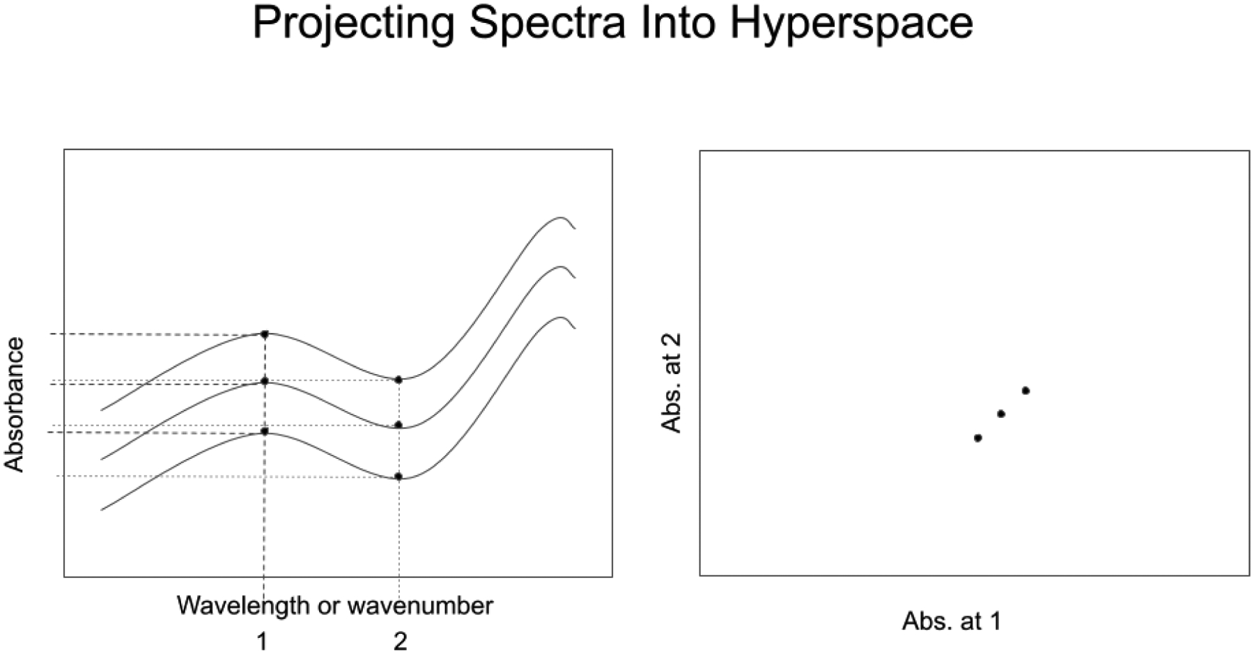
Projecting n spectra at d wavenumbers as n points in a d-dimensional hyperspace. (n=3, d=2)

In Figure 1, the spectra on the left are recorded at 2 wavenumbers, designated 1 and 2. The space depicted on the right shows three points corresponding to the three spectra. The displacement of each point along axis 1 and axis 2 represent the absorbance values recorded in the spectra on the left at wavenumber 1 and wavenumber 2. The spectra are identical except for a constant absorbance baseline offset at each individual wavenumber. As a result, the spectral points in the space on the right are displaced the same amount on axis 1 and axis 2, and the points form a line with a slope of 1. Similar spectra will group in similar regions of hyperspace (see Figure 2, in which two groups of spectra appear separated by a distance larger than the scatter inside each group.)

Figure 2.

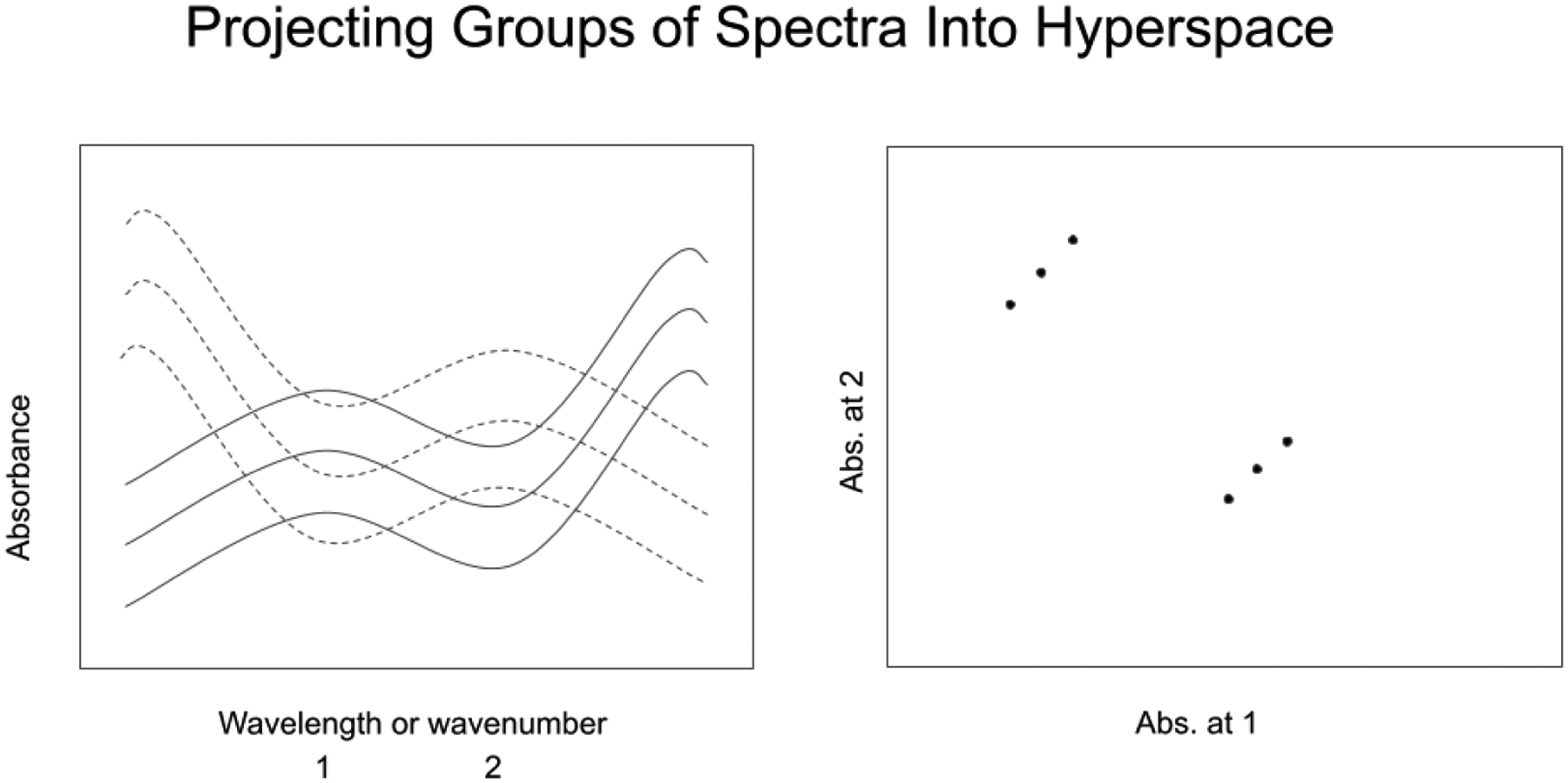
Projecting two groups of n spectra at d wavenumbers as n points in a d-dimensional hyperspace. (n=6, d=2)

The distance from a single spectral point to a group of spectra can be measured in several ways, including in multidimensional standard deviations (SDs) of the group of spectra in hyperspace (measuring in SDs adds the possibility of assigning a probability that one spectrum belongs to a group of spectra). The situation becomes more complicated when attempting to measure the difference between one lot of a drug and another lot when there are multiple vials in each lot group. There is frequently a small amount of variation from lot-to-lot of a drug, resulting in groups that overlap and do not separate well when plotted (see Figure 3).

Figure 3.

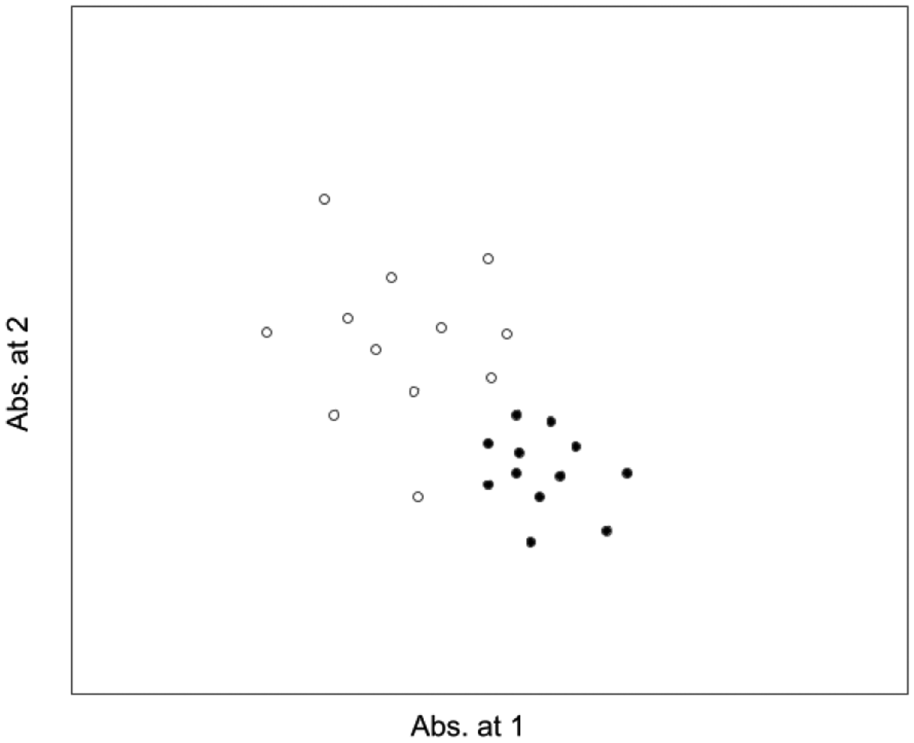
Detecting signals can be complicated even in the case of normally distributed clusters because of overlap of the clusters, different sizes of the clusters, and lack of true normality.

In these cases, it is possible to measure the distance of every single spectrum in one lot to a cluster of other samples in another lot, and this process must be extended to every cluster that exists for that drug. However, this results in a cumbersome number of measurements. More commonly, a subcluster analysis method is used to measure the probability that one cluster was generated from the same process and materials as another overlapping cluster.

Of course, it’s not as easy to visualize hyperspace in actuality. These spectral clusters exist in a hyperspace that often has thousands of dimensions. Under such circumstances the big question becomes, “How are differences between these clusters detected and measured?”

Mahalanobis Distance

The Mahalanobis distance (MD) has been used to measure distances in SDs between data in multidimensional space for almost a hundred years. In an ordinary Euclidean space, variables (e.g. x, y, z) are represented by axes drawn at right angles to each other. The distance between any two points can be measured with a yardstick. For uncorrelated variables with equal SDs, the Euclidean distance equals the MD. However, if two or more variables are correlated, the axes are no longer at right angles. If the standard deviations of the variables are not equal, more than one yard stick is needed. In addition, if there are more than three variables, they cannot be plotted in regular 3D space at all. The MD Is an attempt to solve this measurement problem, as it measures distances between points, even correlated points for multiple variables with unequal SDs.

The MD measures distance relative to the centroid, the central point of a cluster that can be thought of as an overall mean for the multivariate data (see Figure 4). The centroid is a point in hyperspace where all means from all variables (absorbances at different wavenumbers for the DQS) intersect. The larger the MD, the farther away from the centroid the data point lies. The MD is often used to find outliers in hyperspace, which designate unusual combinations of data at two or more variables. In effect, the MD is like a rubber yardstick, whose length (stretch) depends on the direction in which it is oriented.

Figure 4.

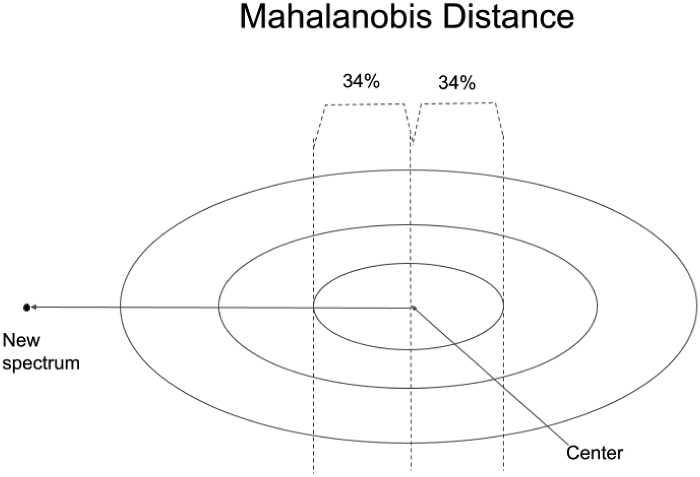
The Mahalanobis distance acts like a “rubber yardstick” whose stretch depends on the direction of the new spectral point. In a normal distribution on SD forms a central 68% confidence interval. The MD works for symmetric, normally distributed data in hyperspace.

BEST (Bootstrap Error-Adjusted Single-sample Technique)

The BEST calculates distances in multidimensional, asymmetric, nonparametric central 68% confidence intervals in spectral hyperspace (equivalent to SDs for normally distributed data, see Figure 5)(Dempsey, 1996). Like the MD, the BEST metric can be thought of as a “rubber yardstick,” but this time with a nail at the center (the mean). The stretch of the yardstick in one direction is independent of the stretch in the other direction. This independence enables the BEST metric to describe odd shapes in spectral hyperspace (spectral point clusters that are not multivariate normal, such as the calibration spectra of many biological systems). BEST distances can be correlated to sample composition to produce a quantitative calibration, or used qualitatively to identify outliers or spectra in similar regions of hyperspace. The BEST automatically detects samples and situations unlike any encountered in the original calibration, making it more accurate in chemical investigation than typical regression approaches to near-IR analysis. The BEST produces accurate distances even when the number of calibration samples is less than the number of wavelengths used in calibration, in contrast to other metrics like the Mahalanobis that require matrix factorization. The BEST is much faster to calculate as well (O(n) instead of the O(n³) required by matrix factorization.)

Figure 5.

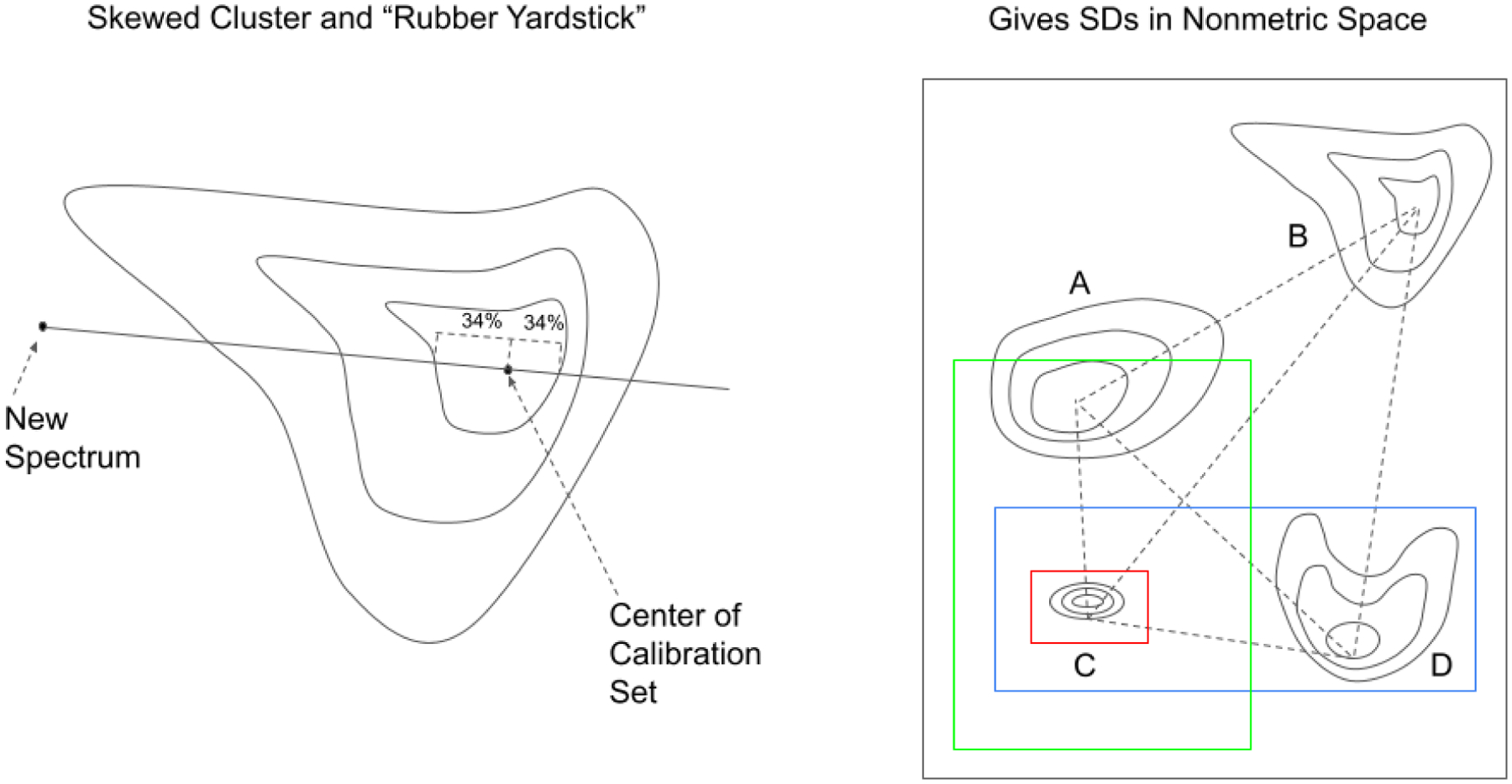
The BEST distance acts like a “rubber yardstick with a nail in it.” The nail is located at the center (mean) of the data cluster. Because the BEST is anchored at the center, the stretch of the yardstick in one direction is independent of the stretch in the opposite direction. For this reason, the BEST is able to model skewed distributions as well as symmetric distributions.

Figure 6 shows how simulated spectral data were created to compare the accuracy and precision of the MD and BEST metrics. Known distributions were created in hyperspace, both spheroidal and ellipsoidal. Random samples were then drawn from these distributions to create spectral test sets. Replicate trials enabled both accuracy and precision to be determined. A round-the-compass-rose approach was used in which new spectral points were created on the axes and off the axes of the spheroids and ellipsoids. In the data shown below in Figure 6, six compass points were used, arranged as in the left panel, and an MD and BEST distance were measured at each point (Brooks, 2018).

Figure 6.

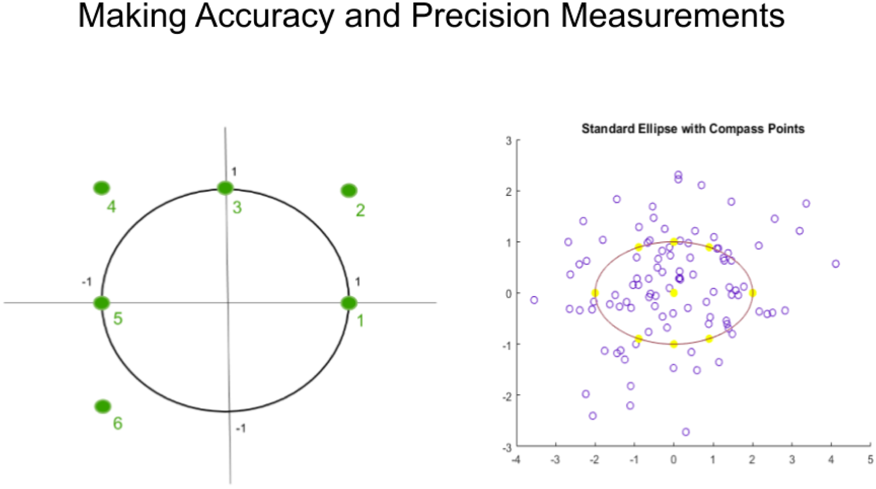
Spheroid and ellipsoid clusters were used to make accuracy and precision measurements.

Because the data were drawn from a known distribution, the true (or actual) distance of each compass rose point is known. This true distance is shown as the red line in Figure 7. The MD is shown in green, and the BEST distance is shown in blue. This example favors the MD because there are 50 times more samples than there are wavenumbers in the example. Under such ideal conditions, the MD metric and the BEST metric produce almost identical results. The deviation from the true or actual distance is created by the random sample drawing from the known distribution, not the performance of the MD or BEST metric. Redrawing a new random sample creates an example with different biases at each dimension but equivalent precision. The point is that when many more samples are available than wavenumbers, the BEST and MD results are very similar. However, in practice, such large numbers of samples are difficult to gather and process. The FTNIR spectrometer records data at 1557 wave numbers. To have 50 times more drugs than wavenumbers would require DQS to scan 77,850 vials of one drug.

Figure 7.

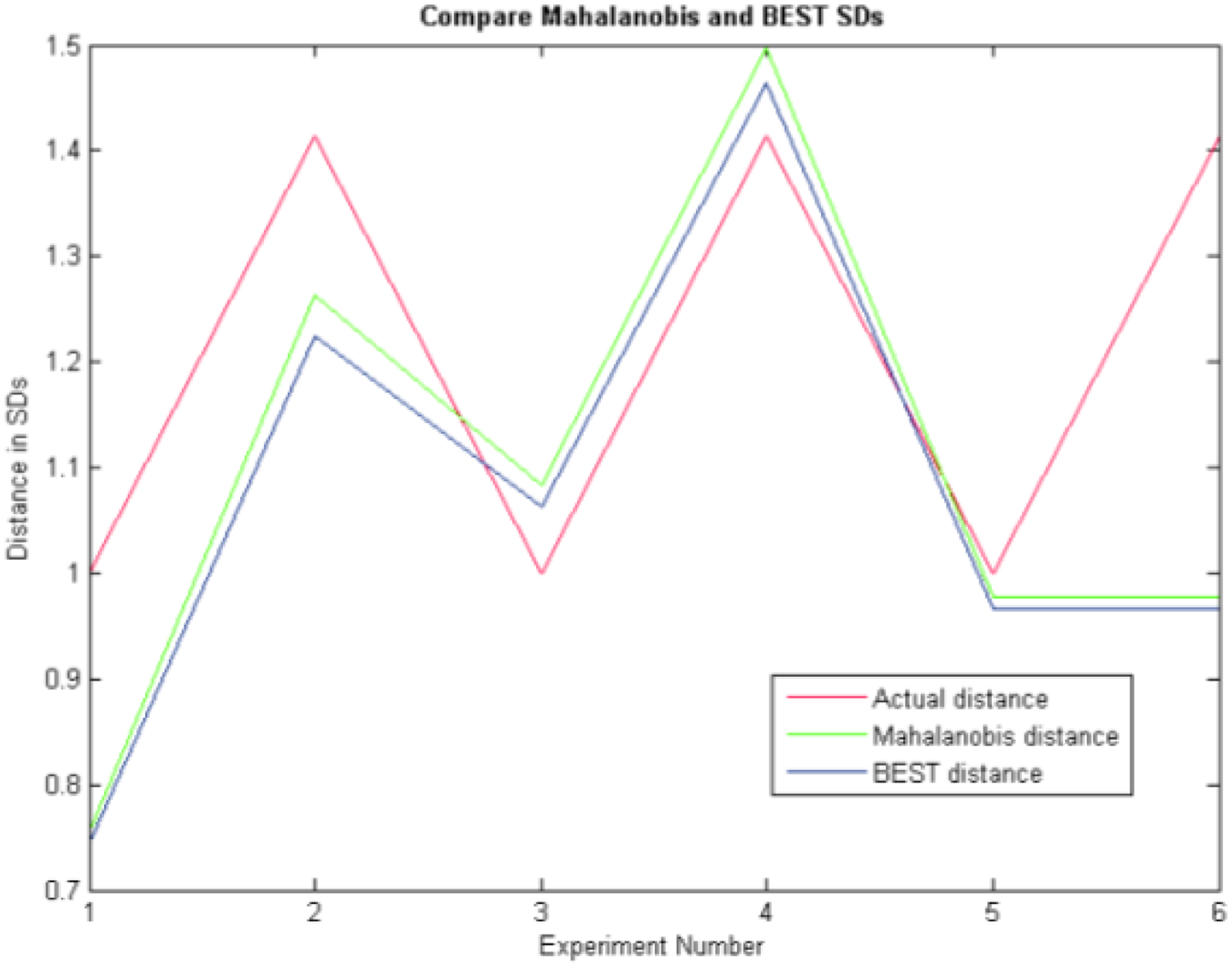
When the number of samples greatly exceeds (50x in this example) the number of wavenumbers at which data are recorded (or PCs), the Mahalanobis metric and the BEST metric produce almost identical results.

In the vast majority of cases, there are absorbances recorded many more wavenumbers than there are vials of drug available. In such cases, it is impossible to calculate an MD conventionally because the data matrix is not invertible or factorable. In order to use the MD the data must be compressed into a much smaller hyperspace using techniques like principal axis transformation. Even then, it can be difficult to collect more drug vials than principal components.

Figure 8 (left) gives accuracy, precision, and execution time for the MD and BEST metrics for the opposite extreme from Figure 7. In this case, the number of vials exceeds the number of wavenumbers by only two (Brooks, 2018). Error in the reproducibility of results from the MD rap leave rises to approximately 1000%. The accuracy is even worse, with the bias rising to thousands of percent error. The error in accuracy continues to climb as the number of wavenumber dimensions increases, while the increase in Relative Standard Deviation (RSD) is not as rapid.

Figure 8.

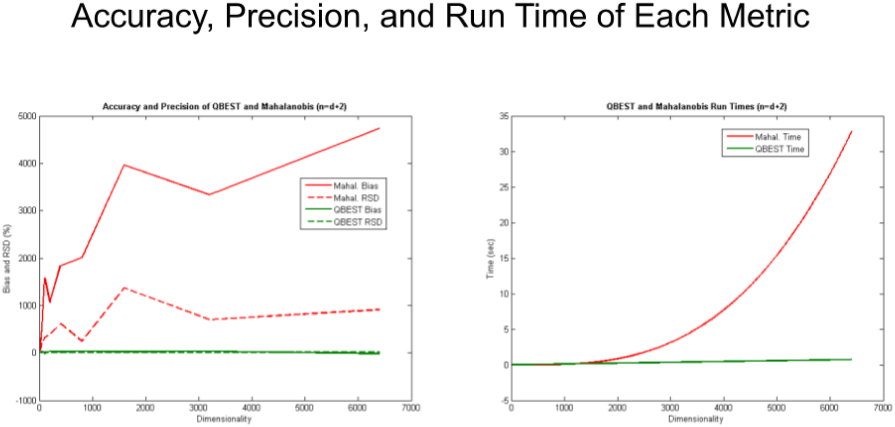
The number of samples exceeds the number of wavelengths by only two, the BEST metric is thousands of percent more accurate and precise than the MD metric. Plus, for any relationship between samples and wavenumbers, the BEST metric is O(d²) faster to compute.

Figure 8 (right) gives the CPU (Central Processing Unit) execution time of the BEST and MD metrics over the same number of dimensions or wavenumbers used in Figure 8 (left) (Brooks, 2018). The execution time of the BEST algorithm increases only linearly and much more slowly than the increase in the MD metric. Computationally, the BEST metric is order of d (where d equals the number of dimensions, O(d) ) while the MD metric is order of d cubed (O(d³)). Figure 8 demonstrates why the BEST metric is such a computational advance and allows much bigger problems to be tackled than conventional approaches like the Mahalanobis distance.

BEST Subcluster Detection

As noted earlier, in typical near-infrared multivariate statistical analyses, samples with similar spectra produce points that cluster in a certain region of spectral hyperspace. These clusters can vary significantly in shape and size due to variation in freeze drying, sample packing, particle-size distributions, component concentrations, and drift with time. These factors, when combined with discriminant analysis using simple distance metrics, produce a test in which a result that places a particular point inside a particular spectral cluster does not necessarily mean that the point is actually a member of the cluster. Instead, the point may be a member of a new, slightly different spectral cluster that overlaps the first. A new cluster can be created by factors like low-level contamination, moisture uptake, or process drift. An extension of the BEST, called FSOB (Fast Son of BEST) can be used to set nonparametric probability-density contours inside spectral clusters as well as outside (Lodder, 1988), and when multiple points begin to appear in a certain region of cluster-hyperspace the perturbation of these density contours can be detected at an assigned significance level using r values, and visualized using quantile-quantile (QQ) plots. The detection of unusual samples both within and beyond 3 SDs of the center of the training set is possible with this method. Within the ordinary 3 SD limit, however, multiple instances are needed to detect unusual samples with statistical significance.

When there is more than a single sample, it is possible that the larger sample of data points from the test set could produce a new cluster with a different mean and standard deviation that overlapped the training set. When it is possible to collect a sufficiently large sample of these spectra, it is possible to detect a signal even inside the nominal three standard deviation limit from the cluster center on single points. Different configurations of clusters lead to different patterns in the Quantile-Quantile (QQ) plots and different effects on the correlation coefficients calculated on the QQ plots. The basic configurations and observed effects are discussed below.

Pure Location Difference

The FSOB algorithm calculates 2 integrals numerically, the integral from the center of the training set out in all directions, and the integral from the center of the training set and the union of the training set and test set (see Figure 9). If the training set and the test sets were identical, this would be the same as calculating the integral from the center of the training set out in all directions twice, and the correlation (r) between the two integrals would be 1. In Figure 9, the two synthetic data clusters were designed to be exactly the same size and shape, and differ only in their location (the groupmean, or center).

Figure 9.

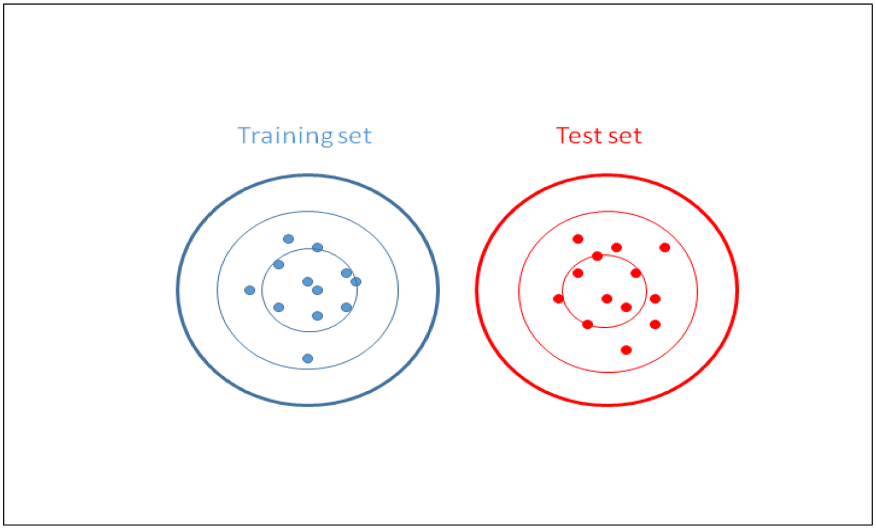
A pure location difference between the training set and the test set. Those two populations are identical except for their locations (centers). The shapes of the distributions have been arbitrarily selected to be circles (or hyperspheres in hyperspace of larger dimension) with the same standard deviation in all directions. Probability density contours are drawn around the clusters.

The CDF (Cumulative Distribution Function, the integral of a Probability Distribution Function, or PDF) plots corresponding to the pure location difference situation in Figure 9 appear in Figure 10. The two sigmoidal integration curves have different locations and their centers are shown with the vertical black lines in Figure 10. The color code is the same as Figure 9, with blue being the training set integral or CDF, and red being the test set CDF. (Order statistics are sample values placed in ascending order. The k^th order statistic of a statistical sample is equal to its k^th-smallest value.)

Figure 10.

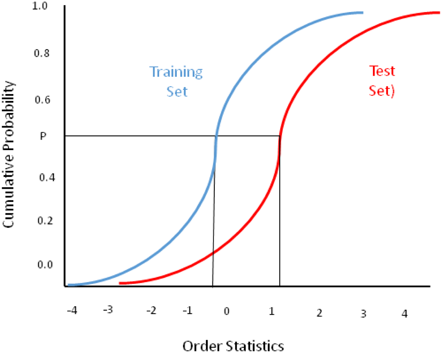
CDF plots of the training set (blue) and test set (red). The x axis values represent the normalized Euclidean distances of each point in SDs from the center of the training set.

The QQ (quantile-quantile) plot in Figure 11 is formed by plotting pairs of points at each cumulative probability in Figure 10. The gray lines in Figure 10 show how these cumulative probabilities are selected and plotted, starting at zero and moving toward one.

Figure 11.

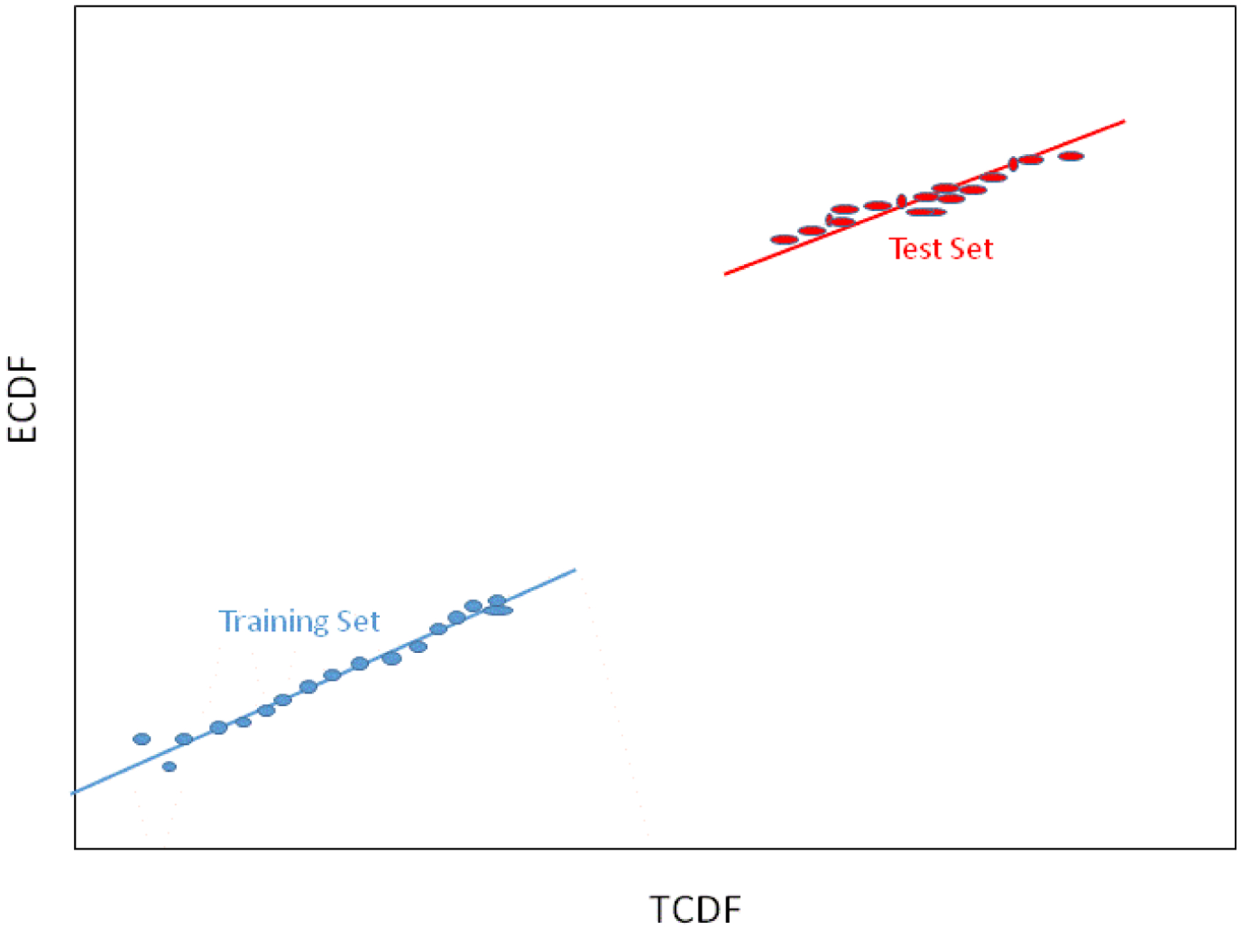
QQ Plot. A correlation coefficient calculated for the QQ plot gives an indication of how well the two distributions (training set and test set) match. A correlation coefficient of r=1 indicates matching distributions. A 98% confidence limit on r is typically used to detect a match. If a measured r is greater than the 98% limit, the two distributions are said to match.

When the underlying probability distribution is Gaussian, a QQ plot is called a normal probability plot and the slope of the line segments reveals the standard deviation of the distribution generating the line segment, while the intercept of the line reveals the mean of the distribution generating that line segment. Because there is only a location difference in the two distributions in this example, the slopes of the lines are the same and only the intercepts differ.

A correlation coefficient can be calculated from this QQ plot and used to determine how well the TCDF matches the ECDF, as shown in Figure 12. As the training set is moved away from a test set of the same size, the correlation coefficient between the two integrals falls. Soon it drops below a 98% confidence limit (or any other confidence level desired) set on bootstrap replicates of the training set. At that point the two groups can be said to be statistically different At the chosen level of significance.

Figure 12.

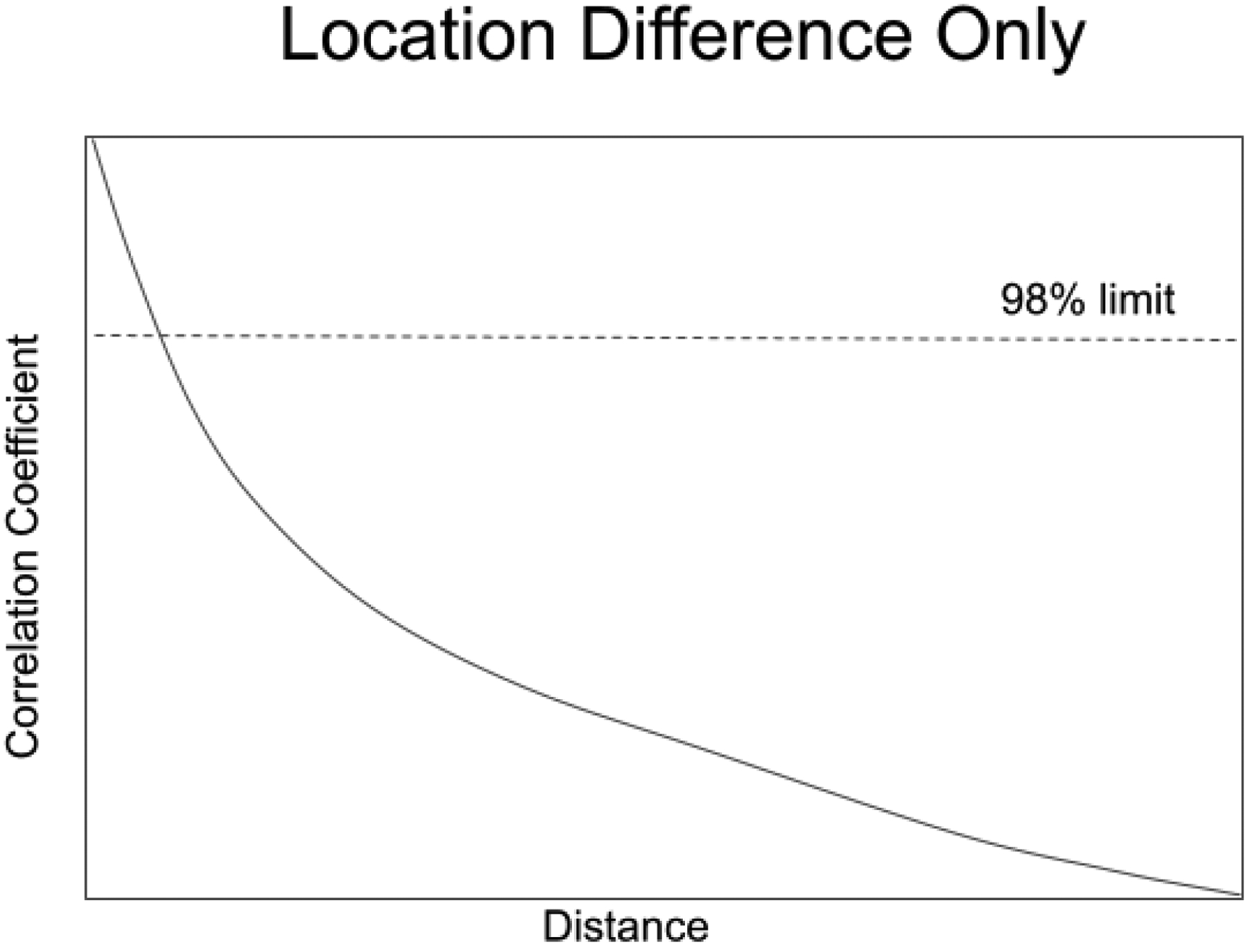
The effects of a pure location difference on the correlation coefficient calculated from a QQ plot. The horizontal dashed line represents a 98% limit on the training set calculated with the use of validation samples.

Pure Scale Difference: Training Set Larger

Another situation that can arise is when the centers of two groups of spectra share the same location (group mean) in hyperspace, but differ in scale (spectral variability). Figure 13 shows the situation in which the training set is larger in scale than the test set, but the centers of each set still share the same exact location in space (Figure 13, left). In such cases, the QQ plot develops three segments with different slopes, see Figure 13, center). The slopes of the line segments in the QQ plot are still a function of the scale of the groups, so the training set segments have a larger slope than the test set segment. As the test set shrinks in scale (spectral variability) relative to the training set, the slope of the test set segment is reduced and the correlation coefficient through the QQ plot falls (see Figure 16, right). The scale factor in Figure 13 (right) is the multiplier by which the training set is larger than the test set.

Figure 13.

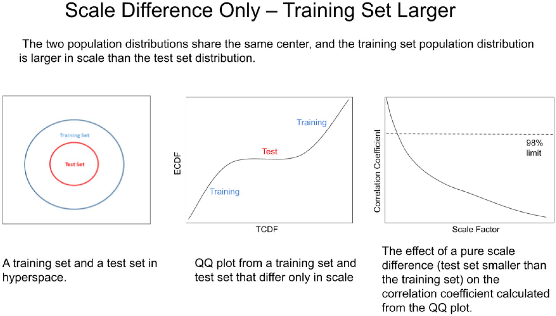
The effects of a pure scale difference on the correlation coefficient calculated from a QQ plot. The scale represents the spectral variability. In this instance the test set spectra are more reproducible than the training set spectra.

Figure 16.

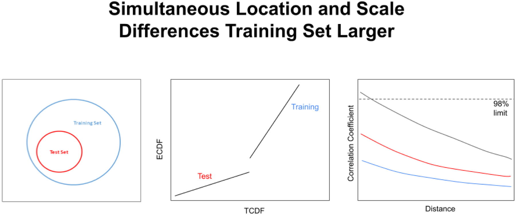
The effects of simultaneous location and scale differences (left) on the correlation coefficient calculated from the QQ plot when the training set is larger than the test set scale. If the location difference is large enough it is even possible for a break to appear in the QQ plot curve (center). The colors of the lines on the right correspond to the scale factors 2 (black curve), 5 (red curve), and 10 (blue curve). When the scale factor is large enough (between 2 and 5 in the graph on the right), the training set is always differentiated from the test set even when the two sets share the exact same center in hyperspace.

Pure Scale Difference: Training Set Smaller

The opposite situation can also occur, in which the training set is smaller in scale than the test set (see Figure 14). In pharmaceuticals a smaller training set is actually more often the case than having a training set larger in scale than the test set. In the same way, drug standards often have lower variability than production vials. As in Figure 13, a small difference in scale factor is enough to cause a statistically significant change in correlation coefficient through the QQ plot.

Figure 14.

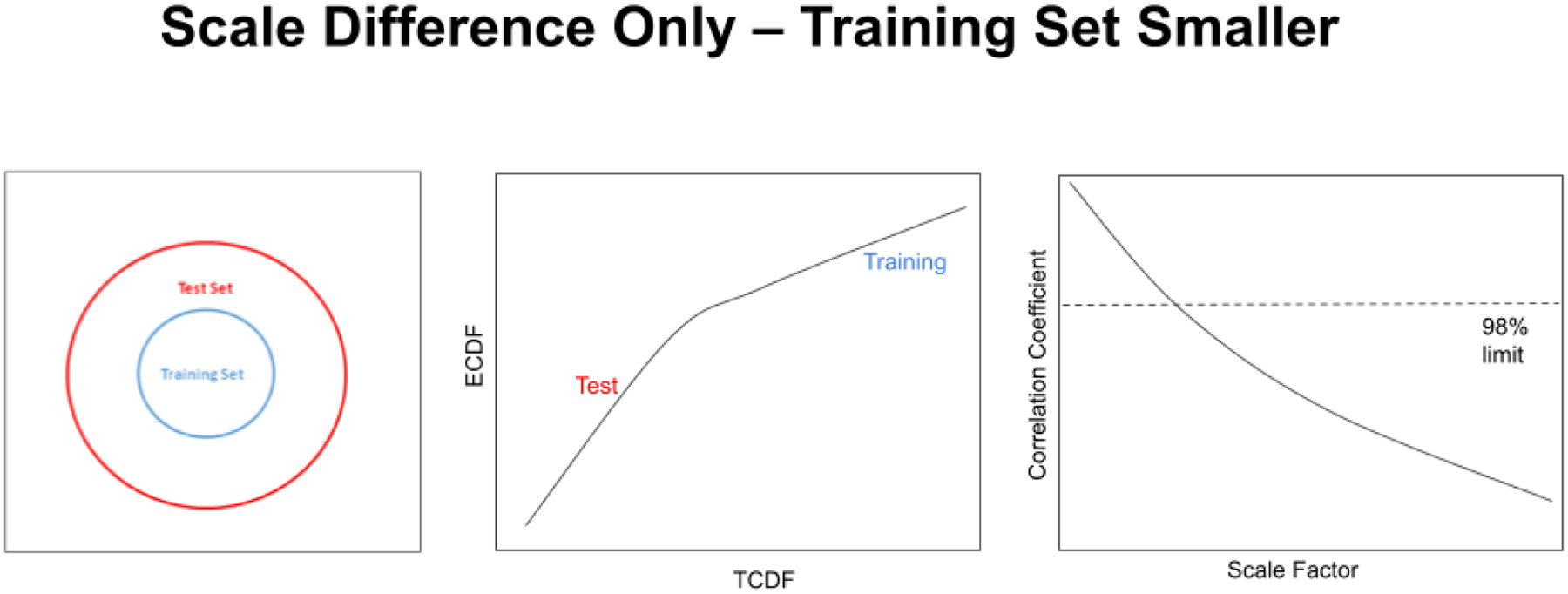
A QQ plot from the subcluster detection method corresponding to the pure scale difference situation. The test set is larger in scale than the training set (left), and a test set forms the lower line with the larger slope in the figure (center). The bend in the line is slight because the difference between the two set scales is only a factor of 2.5. As the training set shrinks in scale relative to the test set, the slope of the training set segment is reduced and the correlation coefficient through the QQ plot falls (right). The scale factor is the multiplier by which the test set is larger than the training set.

Simultaneous Location and Scale Differences: Training Set Smaller

In actual application, however, it is more typical to see simultaneous differences in location and scale in spectral groups when the two groups are different. Under these conditions the subcluster detection test becomes very sensitive to changes between the training set and the test set of spectra.

Figure 15 (left) shows the situation in which there are simultaneous differences in location and scale between the spectral groups, and the training set is the smaller group. This situation results in a bend in the QQ plot line, with the line segment with the highest slope corresponding to the test set and the line segment with the lower slope corresponding to the training set (see Figure 15 center). If the location difference is large enough it is even possible for a break to appear in the QQ plot curve. Figure 15 (right) shows 3 example correlation coefficient plots for the test set larger than the training set (scale factor 2 [black curve], 5 [red curve], and 10 [blue curve]) vs.increasing distances between the centers of the two groups. As evident in Figure 15 (right), when the scale factor is large enough ( between 2 and 5 in this figure), the training set is always differentiated from the test set even when the two sets share the exact same center in hyperspace.

Figure 15.

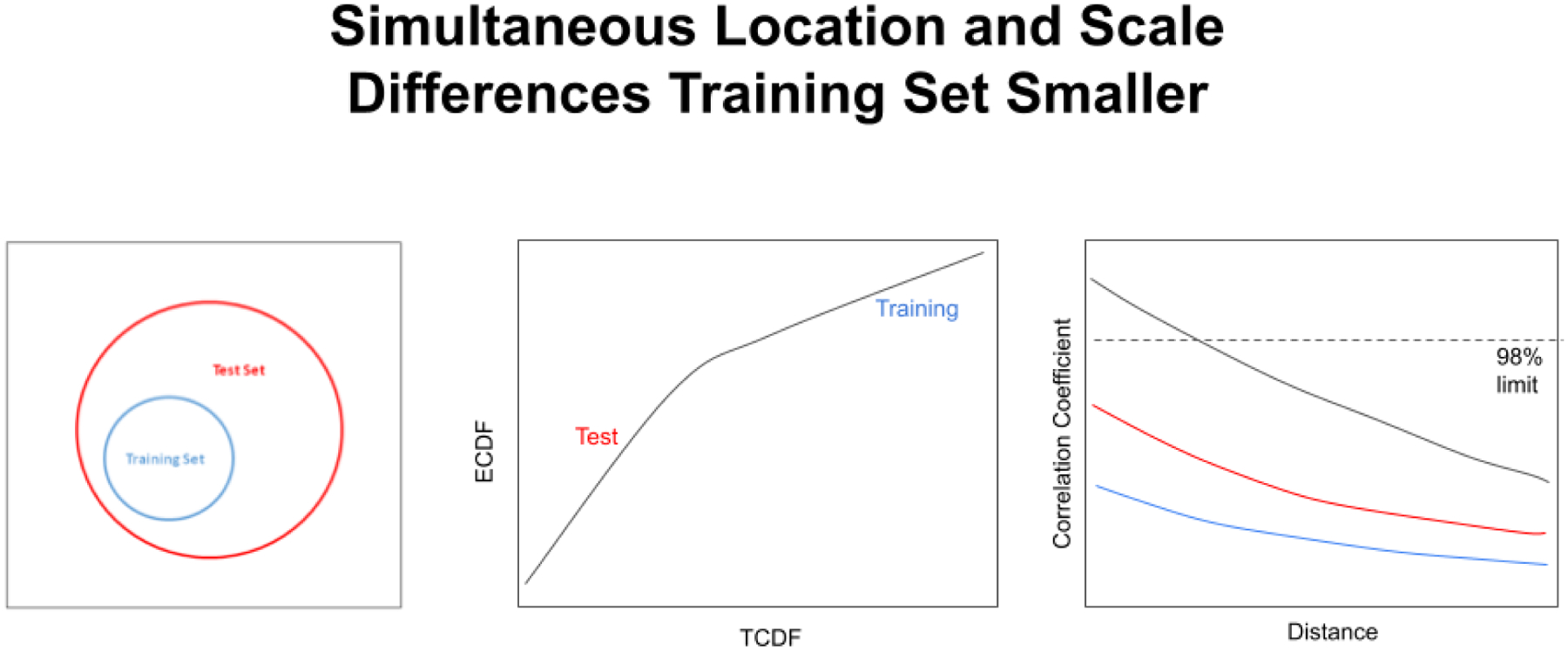
A QQ plot from the subcluster detection method corresponding to the simultaneous location and scale difference situation (left). The test set is a factor of two larger in scale than the training set, and the two set centers are 0.5 standard deviation of the training set apart (center). The colors of the lines correspond to the scale factors 2 (black curve), 5 (red curve), and 10 (blue curve). When the scale factor is large enough ( between 2 and 5 in the graph on the right), the training set is always differentiated from the test set even when the two sets share the exact same center in hyperspace.

Simultaneous Location and Scale Differences: Training Set Larger

It is also possible for simultaneous location and scale differences to exist when the training set is larger in scale than the test set (see Figure 16, left). This situation can arise, for example, when a series of batches are created for a phase 3 clinical trial to capture the possible process variations in their proposed “CMC box” for the FDA, and then production samples cluster in a smaller area of hyperspace. From an operations standpoint, this may actually be the ideal case for production, because minor process variations can still produce approved products. Unfortunately, a training set larger than the test set is sometimes not observed in production.

Like simultaneous location and scale differences when the training set is smaller, simultaneous location and scale differences when the training set is larger can cause a break to appear in the QQ plot curve (Figure 16, center). As the training set and test set move apart and change in scale, the correlation coefficient calculated through the QQ plot (Figure 16, center) drops lower and lower (Figure 16, right).

QQ plots and the subcluster detection algorithm are important because these analyses take place in a hyperspace of thousands of dimensions, and it is very difficult to visualize differences between spectral clusters in such high dimensional hyperspaces. Draftsman’s plots become impractical. Mahalanobis distances become inaccurate. Transformation to principal axes may downweight a wavenumber that contains the essential impurity information needed. For reasons like these, the BEST metric and the subcluster detection BEST were selected for use in the Drug Quality Study.

Principal Component Analysis (PCA)

Transformation to principal axes is a data reduction technique (see Figure 17). The transformation concentrates the variation in the spectra into orthogonal axes. Principal component analysis (PCA) is the process of computing the principal components (PCs) of a dataset and using them to execute a change of basis (change of coordinate system) on the data, usually employing only the first few principal components in analysis and disregarding the rest (Joliffe, 2016). PCA is used in exploratory data analysis and in constructing predictive models. PCA is commonly utilized for dimensionality reduction by projecting each data point onto only the first few principal components to obtain lower-dimensional data while preserving as much of the original variation in the data as possible. The first principal component is the direction axis that maximizes the variance of the projected data. The second principal component is the direction of the largest variance orthogonal to the first principal component. Decomposition of the variance typically continues orthogonally in this manner until some residual variance criterion is met. Plots of PC scores help reveal underlying structure in data.

Figure 17.

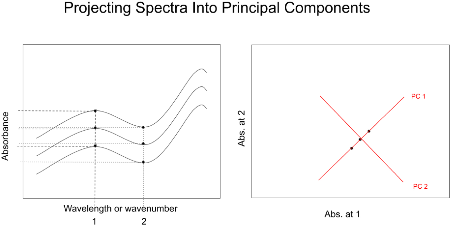
Spectral data values can be represented as wavenumber data or principal component scores. Spectral absorbance data at each wavelength or wavenumber (Figur, left) are encoded as displacements on orthogonal absorbance axes. In PCA (right), the original coordinate axes are translated to the center of the data, and then rotated until the first PC (PC 1) aligns with the largest variation in the data points. The second PC is orthogonal to the first. In 3 or more dimensions, PC 2 is rotated orthogonally around PC 1 to align with the next largest variation in the data points.

Application

Example process appearing in a state of control

Dantrolene

In a previous inquiry, several different lots of dantrolene vials were screened by DQS. The spectra obtained from the vials clustered together with no apparent subclusters or outliers on PCs 4, 5, and 6 (see Figure 18). (Isaacs, 2023a) (This observation underscores the importance of examining all of the major principal components when using principal components of spectra.)

Figure 18.

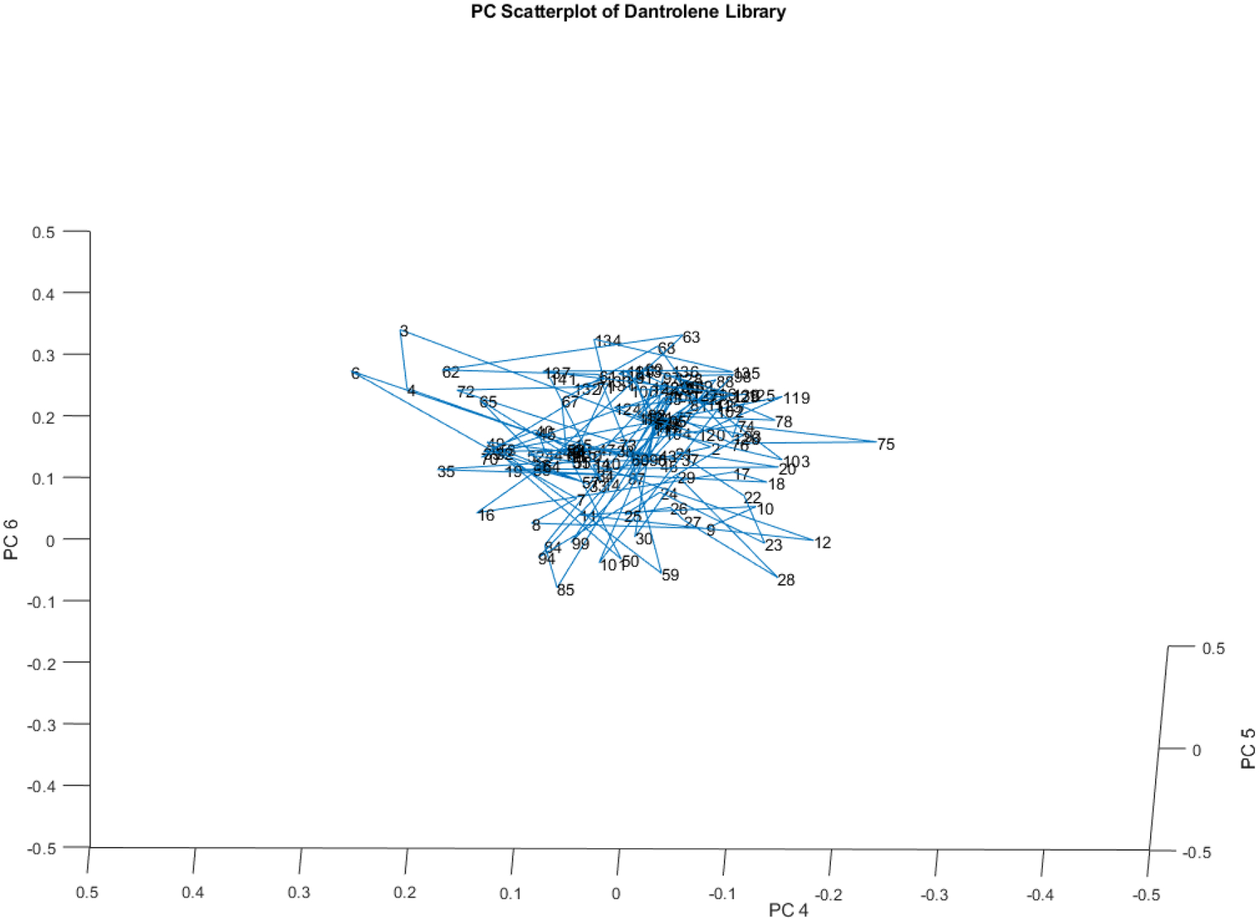
PC plot of spectra of several lots of dantrolene sodium.

No single vials or groups of vials appeared to separate from the main cluster, even though the spectra were not identical. This sort of variation over time in sample spectra is typical of processes operating in a state of good control.

Example process appearing out of control

Abatacept-Maltose

A process that usually produces very similar samples but occasionally produces a sample unlike the rest may be out of a state of control (see Figure 19). Most of the 132 vial spectra from these 34 lots of abatacept-maltose cluster in an ellipsoid in the middle of Figure 19. However, a few spectra (vials 10, 18, 57, 114, 121) skew away from the main ellipsoid.

Figure 19.

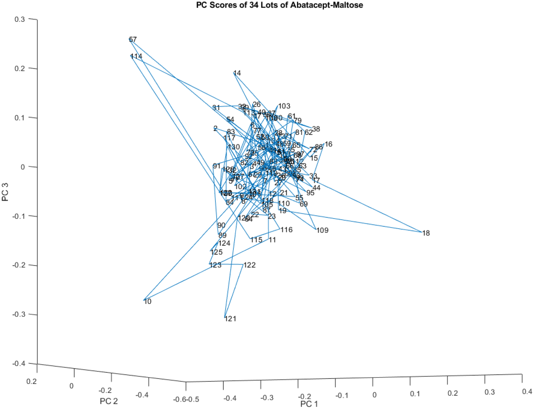
PC scores scatter plot for 132 vials of abatacept-maltose in the spectral library from 34 lots for PC 1, 2, and 3. Vial 57 is 5.6 SDs from the center of the spectral library.

Even in a well controlled process a few samples (e.g. 2 or 3%) will appear to be outliers. When that number gets higher (e. g., 10%), additional investigation into the process control may be indicated.

Example of potential formulation changes

Remifentanil

Sometimes a dramatic change in spectra is detected in lots of a drug that are supposed to be the same. In another study, the DQS detected two distinct groups of chemicals in 90 vials of remifentanil (see Figure 20). The 2 groups of spectra were 50.3 SDs apart using the subcluster detection test (Isaacs, 2023b).

Figure 20.

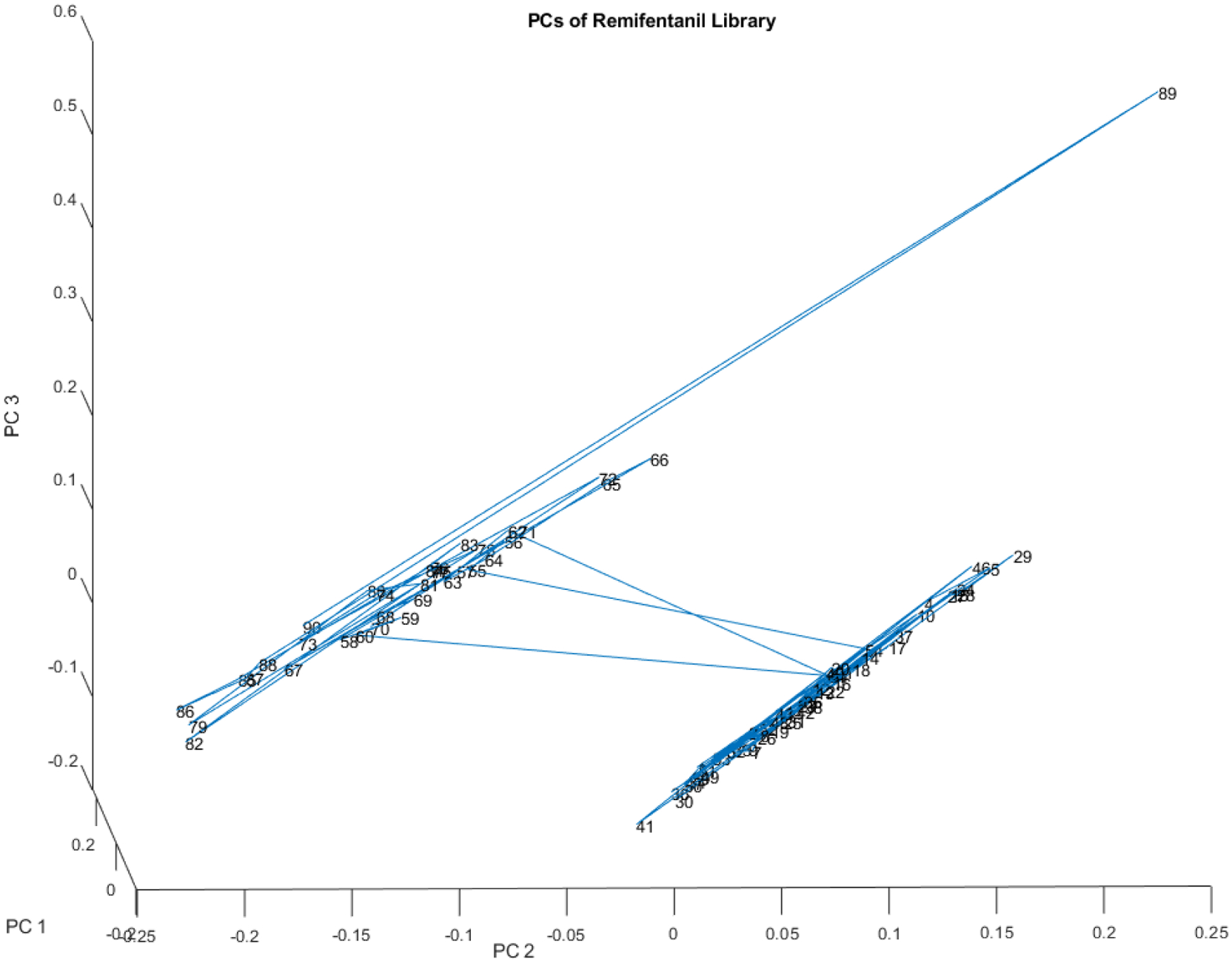
PC score plot of the spectra of the 90 vials in the remifentanil library. The group on the right with more spread contains 35 vials, while the tighter group on the left contains 55 vials. The 2 groups of spectra are 50.3 SDs apart using the subcluster detection test (r_tn=0.99, r_tst= 0.86).

Conclusion

This assessment of subcluster detection in analytical chemistry suggests a nonparametric approach to address the challenges of identifying specific substances (molecules or mixtures) in large hyperspaces. The paper introduces the concept of subcluster detection, which involves identifying a group of specific substances within a larger cluster of similar samples. The BEST metric is introduced as a more accurate and precise method for discriminating between similar samples compared to the MD metric. The paper also discusses the challenges of subcluster detection in large hyperspaces, such as the curse of dimensionality (Powers, 2022) and the need for nonparametric methods. The proposed nonparametric approach involves using a kernel density estimator to determine the probability density function of the data and then using a quantile-quantile algorithm to identify subclusters. The paper provides examples of how this approach can be used to analyze small changes in the near-infrared spectra of drug samples and identifies the benefits of this approach, such as improved accuracy and precision.

In addition to discussing the proposed nonparametric approach, the paper also provides insights into the importance of subcluster detection in analytical chemistry. The ability to differentiate compounds is critical for developing new materials and drug products, as it allows researchers to identify specific substances and understand their properties. The paper highlights the challenges of subcluster detection in large hyperspaces and the limitations of existing methods, such as the MD metric. The proposed nonparametric approach offers a new method for addressing these challenges and provides a more accurate and precise method for subcluster detection. The MD metric is a common method for measuring distances in hyperspace, but it has limitations. One limitation is that it is not very accurate when there are many dimensions and comparatively few samples (in fact, the number of samples must exceed the number of dimensions in order for the matrix to be factorable). Another limitation is that it can be difficult to interpret the results of the MD metric because it is symmetric and subject to low accuracy and precision depending upon the ratio of samples to dimensions.

The BEST metric is a new method for subcluster detection that addresses the limitations of the MD metric. The BEST metric is more accurate than the MD metric, and it is easier to interpret the results. The BEST metric is also more robust to noise and outliers. Finally, the BEST metric is more rapidly calculated in high dimensional spaces.

References

- Brooks AD Dickerson C & Lodder RA The BEST Approach to the Search for Extraterrestrial Intelligence (SETI), ANZIAM 2018 (Hobart, Tasmania, Australia), Feb. 2018 [Google Scholar]
- Dempsey RJ, Davis DG, Buice RG Jr, & Lodder RA (1996). Biological and medical applications of near-infrared spectrometry. Applied Spectroscopy, 50(2), 18A–34A. [Google Scholar]
- Isaacs JT, Almeter PJ, Henderson BS, Hunter AN, Platt TL, & Lodder RA (2023 a). Spectrometric Analysis of Dantrolene Sodium. Contact in context, 2023a. [DOI] [PMC free article] [PubMed] [Google Scholar]
- Isaacs JT, Almeter PJ, Henderson BS, Hunter AN, Platt TL, & Lodder RA (2023 b). Spectrometric Analysis of Process Variations in Remifentanil. Contact in context, 2023b. [DOI] [PMC free article] [PubMed] [Google Scholar]
- Jolliffe IT, & Cadima J (2016). Principal component analysis: a review and recent developments. Philosophical Transactions of the Royal Society A: Mathematical, Physical and Engineering Sciences, 374(2065), 20150202. [DOI] [PMC free article] [PubMed] [Google Scholar]
- Lodder RA, & Hieftje GM (1988). Detection of subpopulations in near-infrared reflectance analysis. Applied spectroscopy, 42(8), 1500–1512. [Google Scholar]
- Powers Jessica, & Shetty Badreesh. What Is the Curse of Dimensionality? Built In. Aug 19, 2022. Retrieved Aug. 4, 2023. [Google Scholar]