Signatures of magnetism control by flow of angular momentum

Abstract

Exploring new strategies to manipulate the order parameter of magnetic materials by electrical means is of great importance not only for advancing our understanding of fundamental magnetism but also for unlocking potential applications. A well-established concept uses gate voltages to control magnetic properties by modulating the carrier population in a capacitor structure^1–5. Here we show that, in Pt/Al/Fe/GaAs(001) multilayers, the application of an in-plane charge current in Pt leads to a shift in the ferromagnetic resonance field depending on the microwave frequency when the Fe film is sufficiently thin. The experimental observation is interpreted as a current-induced modification of the magnetocrystalline anisotropy ΔH_A of Fe. We show that (1) ΔH_A decreases with increasing Fe film thickness and is connected to the damping-like torque; and (2) ΔH_A depends not only on the polarity of charge current but also on the magnetization direction, that is, ΔH_A has an opposite sign when the magnetization direction is reversed. The symmetry of the modification is consistent with a current-induced spin^6–8 and/or orbit^9–13 accumulation, which, respectively, act on the spin and/or orbit component of the magnetization. In this study, as Pt is regarded as a typical spin current source^6,14, the spin current can play a dominant part. The control of magnetism by a spin current results from the modified exchange splitting of the majority and minority spin bands, providing functionality that was previously unknown and could be useful in advanced spintronic devices.

Signatures of magnetism control by the flow of angular momentum are observed in Pt/Al/Fe/GaAs(001) multilayers by the application of an in-plane charge current in Pt.

Main

Spin torque (spin-transfer torque and spin–orbit torque), which involves the use of angular momentum generated by partially or purely spin-polarized currents, is a well-known means for manipulating the dynamic properties of magnetic materials. In structures such as giant magnetoresistance or tunnel magnetoresistance junctions, the flow of a spin-polarized electric current through the junction imparts spin-transfer torques on the magnetization in the free ferromagnetic layer^15–17. In heavy metal (HM)/ferromagnet (FM) bilayers, a charge current flowing in HM induces a spin accumulation at the HM/FM interface and generates spin–orbit torques (SOTs) acting on FM¹⁸. These torques serve as versatile control mechanisms for magnetization dynamics, such as magnetization switching^19,20, domain wall motion^21–23, magnetization relaxation²⁴ and auto-oscillations of the magnetization^25,26. These innovative approaches and their combinations open up a spectrum of possibilities for tailoring magnetic properties with potential implications for technologies such as magnetic random access memories^18,27.

General considerations

Although the impact of spin currents on the orientation of the magnetization M is widely recognized, there have been only a few explicit observations of successful spin-current-driven manipulation of the magnitude of M. Previous work²⁸ has shown that, in a magnetic Ni/Ru/Fe tri-layer in which the two magnetization layers are coupled by an exchange coupling, ultrafast laser-generated super-diffusive spin currents in Ni transiently enhance the magnetization of Fe when the two ferromagnetic layers are aligned parallel and decrease when the two ferromagnetic layers are aligned antiparallel, respectively. This transient effect is limited to low optical excitations because super-diffusive spin currents saturate at high power. To explore the modulation of magnetism by spin current, Fig. 1 shows the process of spin current transfer^{15–17,29–31}. Spin accumulation, generated by a charge current I, contains both transverse and longitudinal spin components with respect to M. It can be generated by the strong spin splitting of the energy band of ferromagnetic metals¹⁷, by spin Hall effect⁶, by orbital Hall effect and by subsequent conversion of the orbital current into a spin current by the spin–orbit interaction in the bulk⁷ as well as by spin Rashba–Edelstein effect (alternatively named inverse spin galvanic effect)⁸ at the interfaces. The incident transverse spin current dephases and is absorbed by M, which gives rise to damping-like spin torques and is responsible for the change in M direction^29,30. After spin transfer and in the spin diffusion length of FM, the exiting spin current is on average aligned with M, and the spin-up electron can fill the majority band when M is along the +z direction (Fig. 1a). Owing to the enhanced exchange splitting of the majority and minority spin bands, this leads to an enhancement of M as well as an increase in the magnetic anisotropies. When M is along the −z direction as shown in Fig. 1b, a decrease in M is expected because of the filling of the minority band and the reduction of the exchange splitting. Similarly, once the polarity of the spin current is reversed by reversing the polarity of I, a decrease or an increase in M is expected if M ∥ +z or M ∥ −z, respectively, as shown in Fig. 1c,d. Therefore, the change in magnetization ΔM by a spin current is expected to be odd with respect to the inversion of either I or M, that is, ΔM(I, M) = −ΔM(−I, M) = −ΔM(I, −M).

Fig. 1. Schematic of the microscopic mechanism of manipulation of magnetism by a spin current.

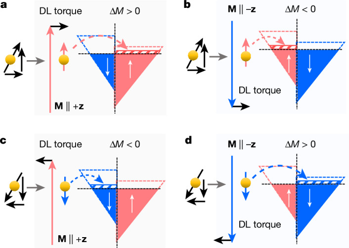
a, The electron spins transmitted into the FM contain both transverse and longitudinal components with respect to M. Owing to exchange coupling, the transverse component dephases and is absorbed by M, which gives rise to the damping-like (DL) SOT and is responsible for changing the direction of M. The longitudinal component of the spin current is on average aligned with M, leading to additional filling of the majority band when M is oriented along the +z direction, and an enhancement of the magnitude M as well as an increase in magnetic anisotropies are expected because of the enhanced exchange splitting of the majority and minority spin energy bands. b, When M is aligned along the –z direction, the spin-polarized electron enters the minority band, which can lead to a decrease in M as well as a decrease in the magnetic anisotropies because of the reduction in the exchange splitting of the majority and minority spin energy bands. c,d, The same as a and b but the polarization of the spin current is reversed, which is expected to reduce M for M ∥ +z (c) and enhance M for M ∥ −z (d).

Ferromagnetic resonance measurements

To prove the above scenario, Pt (6 nm)/Al (1.5 nm)/Fe (t_Fe = 4.5, 2.8, 2.2 and 1.2 nm) multilayers with different Fe thicknesses t_Fe are grown on a single 2-inch semi-insulating GaAs(001) wafer by molecular-beam epitaxy (Fig. 2b, Methods and Supplementary Note 1). The ultrathin Fe films on GaAs(001) allow us to investigate the expected modification of the magnetic properties for two reasons: Fe/GaAs(001) shows (1) very low Gilbert damping α values in the sub-nanometre thickness regime (α = 0.0076 for t_Fe = 0.91 nm) (ref. ³²), and thus it is possible to detect the magnetization dynamics for ultrathin samples and (2) strong interfacial in-plane uniaxial magnetic anisotropy (UMA), which is advantageous for the detection of the spin-current-induced modification of magnetic anisotropies. The UMA originates from the anisotropic bonding between Fe and As atoms at the GaAs(001) surface³³, in which the ⟨110⟩ orientations are the magnetic easy axis (EA) and the $⟨\overline{1}10⟩$ orientations are the magnetic hard axis (HA) (Fig. 2c). We perform time-resolved magneto-optical Kerr microscopy measurements with out-of-plane driving field to characterize both the static and dynamic magnetic properties of Fe under the influence of spin currents generated by applying a charge current in Pt (Fig. 2a and Methods).

Fig. 2. Measurement set-up, device and modification of linewidth by charge current.

a, Schematic of the device for the detection of ferromagnetic resonance by time-resolved magneto-optical Kerr microscopy. b, Schematic of the Pt/Al/Fe/GaAs(001) structure. c, Diagram of crystallographic axes with EA and HA along the ⟨110⟩ and $⟨\overline{1}10⟩$ orientations. d, FMR spectra for different d.c. currents I measured at f = 12 GHz and φ_I–H = 90^o, where φ_I–H is the angle between the magnetic field and the current direction as shown in the inset. The solid lines are the fits. e, FMR linewidth as a function of d.c. current for φ_I–H = ±90^o; solid lines are the linear fits from which the modulation amplitude d(ΔH)/dI is obtained. Error bars represent the standard error of the least squares fit of the V_Kerr(H) traces in d. f, φ_I–H dependence of d(ΔH)/dI. Error bars represent the standard error of the least squares fit of the I–ΔH traces in e. The solid line is the calculated result when taking into account the in-plane magnetic anisotropies of Fe (see Methods).

Source Data

Typical ferromagnetic resonance (FMR) spectra for t_Fe = 2.2 nm and for I ∥ [110] are shown in Fig. 2d. A clear modification of the FMR spectrum is observed. By fitting the curves with the combination of symmetric and an anti-symmetric Lorentzian (Methods), the resonance field H_R and the full width at half maximum ΔH are obtained.

Modification of the linewidth

The dependence of ΔH on I for φ_I–H = ±90° is shown in Fig. 2e, where φ_I–H is the angle between I and the magnetic field H (Fig. 2d, inset). A linear behaviour with opposite slopes for φ_I–H = ±90^o shows the presence of the damping-like SOT, confirming previous reports²⁴. To extract the modification of the linewidth, the I dependence of ΔH is fitted by

$$\mathrm{\Delta }H={\mathrm{\Delta }H}_0+\left[\mathrm{d}\left(\mathrm{\Delta }H\right)/\mathrm{d}I\right]I+c_1{I}^2.$$ 1

Here ΔH₀ is ΔH for I = 0, d(ΔH)/dI quantifies the modification of linewidth by the spin current and c₁ accounts for possible Joule heating effects on ΔH. A detailed measurement of d(ΔH)/dI as a function of φ_I–H shows that d(ΔH)/dI varies strongly around HA. The angular dependence can be well fitted by considering an effective damping-like SOT efficiency ξ of 0.06 (Methods). The weaker damping-like torque, generated by the Bychkov–Rashba-like and Dresselhaus-like spin–orbit interactions at the Fe/GaAs interface, plays a negligible part in the linewidth modulation³⁴. As the angular dependence of d(ΔH)/dI can be well fitted by conventional SOTs^18,35, that is, equation (10) in Methods, there is no need to consider other higher order SOTs³⁶.

Modification of the ferromagnetic resonance field

Having identified the modification of ΔH, we now focus on the modification of H_R, which is related to the magnetization and magnetic anisotropies. Figure 3a,b shows the I dependence of H_R for t_Fe = 2.8 nm measured at selected frequencies f for H applied along EA and HA to avoid magnetic dragging effects^32,34. As shown at the top of each panel, the current is applied along the [100] orientation, and the direction of spin σ is along the [010] orientation with equal projections onto the [110] and $\left[\overline{1}10\right]$ orientations. Therefore, this geometry allows a precise comparison of the current-induced modification of H_R between the [110] and $\left[\overline{1}10\right]$ orientations in the same device. For M ∥ [110] (Fig. 3a), all the H_R–I traces show a positive curvature, whereas for M ∥ $\left[\overline{1}10\right]$ (Fig. 3b), traces with a negative curvature are observed. The positive and negative curvatures along [110] and $\left[\overline{1}10\right]$ orientations are because Joule heating reduces the magnetization and thus the UMA, resulting in an increase in H_R along [110] but a decrease in H_R along $\left[\overline{1}10\right]$. Apart from the symmetric parabolic dependence induced by Joule heating, a linear component in the I dependence of H_R is also observed because H_R(−I) ≠ H_R(+I) holds. Note that for M along both EA and HA, H_R(−I) > H_R(+I) holds for all frequencies. As t_Fe is reduced to 1.2 nm, the I dependence of H_R along the EA is similar to the one with t_Fe = 2.8 nm and H_R(−I) > H_R(+I) still holds (Fig. 3c). However, for M ∥ $\left[\overline{1}10\right]$ (Fig. 3d), the relative magnitude of H_R(−I) and H_R(+I) strongly depends on f, that is, H_R(−I) < H_R(+I) holds for f = 12.0 GHz; H_R(−I) ≈ H_R(+I) holds for f = 14.0 GHz but H_R(−I) > H_R(+I) holds for f = 16.0 GHz. The frequency-dependent shift of H_R indicates that the magnetic properties of Fe are modified by the spin current for thinner samples, an observation that has not been reported before, to our knowledge.

Fig. 3. Modification of resonance field.

a, I dependence of H_R measured at selected frequencies for H along [110] for t_Fe = 2.8 nm. b, The same as a but for H along $\left[\overline{1}10\right]$. c,d, The same plots as a and b but for t_Fe = 1.2 nm. Error bars represent the standard error of the least squares fit of the V_Kerr(H) traces. The red and blue arrows in each panel are marked to show the relative amplitude of H_R(−I) and H_R(+I). As shown in the top panels, for all the devices, the charge currents are applied along the [100] orientation, and the direction of the spin accumulation σ is along the [010] direction with equal projections onto the [110] and $\left[\overline{1}10\right]$ orientations. This experimental trick allows an accurate comparison of the current-induced modification for the [110] and $\left[\overline{1}10\right]$ orientations in the same device.

Source Data

Modification of the magnetic anisotropies

To quantify the modification of the magnetic anisotropies, the I dependence of the H_R trace is fitted by

$$H_{\text{R}}=H_{\text{R}0}+\left(\mathrm{d}{H}_{\text{R}}/\mathrm{d}I\right)I+c_2{I}^2.$$ 2

Here H_R0 is H_R at I = 0, dH_R/dI quantifies the modification of H_R, and c₂ accounts for Joule heating effects on H_R. The f dependences of dH_R/dI for different orientations of M and different t_Fe are summarized in Fig. 4. For t_Fe = 2.8 nm and M ∥ ⟨110⟩ orientations (Fig. 4a), dH_R/dI is independent of frequency with a positive zero-frequency intercept (about 0.08 mT mA⁻¹) for M ∥ $\left[\overline{1}\overline{1}0\right]$. As M is rotated by 180° to the [110] orientation, the sign of the intercept changes to negative with the same amplitude as the $\left[\overline{1}\overline{1}0\right]$ orientation (around −0.08 mT mA⁻¹). This can be understood in terms of the current-induced Oersted field and/or field-like torque h_Oe/FL, arising from the current flowing in Pt and Al, which shifts H_R. The field-like torque originates from the incomplete dephasing (non-transmitted and/or non-dephased) component of the incoming spin^29,30,37. For M along HA (Fig. 4b), the f-independent dH_R/dI has also opposite zero-frequency intercepts for M ∥ $\left[\overline{1}10\right]$ and M ∥ $\left[1\overline{1}0\right]$ with virtually identical h_Oe/FL value as EA. This confirms that the spin accumulation σ has equal projection onto the ⟨110⟩ and $⟨\overline{1}10⟩$ orientations. As t_Fe is reduced to 1.2 nm (Fig. 4c), the intercept of the f-independent dH_R/dI traces along [110] and $\left[\overline{1}\overline{1}0\right]$ orientations, respectively, increases to about −0.20 mT mA⁻¹ and about 0.20 mT mA⁻¹, respectively. However, as M is aligned along HA (Fig. 4d), the dH_R/dI trace differs significantly from other traces: (1) it is no longer f independent but shows a linear dependence on f with opposite slopes for M along the $\left[\overline{1}10\right]$ and $\left[1\overline{1}0\right]$ orientations, (2) the absolute value of the zero-frequency intercept along HA (about 0.32 mT mA⁻¹) is no longer equal to that along EA (about 0.2 mT mA⁻¹). The f dependence of the dH_R/dI traces cannot be interpreted to arise from the frequency-independent h_Oe/FL and can be explained only by a change in the magnetic anisotropies induced by the spin current.

Fig. 4. Modification of magnetic anisotropies.

a, The f dependence of dH_R/dI for H along the EA ([110] and $\left[\overline{1}\overline{1}0\right]$ orientations). b, The f dependence of dH_R/dI for H along the HA ($\left[\overline{1}10\right]$ and $\left[1\overline{1}0\right]$ orientations). The results in a and b are obtained for t_Fe = 2.8 nm. c,d, Same plots as in a and b but for t_Fe = 1.2 nm. Error bars in each figure (most of them are smaller than the symbol size) represent the standard error of the least squares fit of the I–H_R traces in Fig. 3. The insets show the relative orientations between the current (I ∥ [100], black arrows) and the magnetic field (or magnetization), in which the EA are represented by brown arrows and the HA are represented by green arrows. e, Summary of t_Fe dependence of ΔH_A (ΔH_A = ΔH_K, ΔH_U, ΔH_B) for opposite magnetization M directions, in which the solid symbols represent the M direction and the open symbols represent the −M direction. The inset shows the relative orientations between the charge current I and M.

Source Data

In the presence of the in-plane magnetocrystalline anisotropies, the dependencies of H_R on f along EA $H_{\text{R}}^{\text{EA}}$ and HA $H_{\text{R}}^{\text{HA}}$ are given by the modified Kittel formula³⁴

$$\left\{\begin{array}{c}{\left(\frac{2\mathrm{\pi }f}{\gamma }\right)}^2={\mu }_0^2\left(H_{\text{R}}^{\text{EA}}+H_{\text{K}}+\frac{H_{\text{B}}}{2}\right)\left(H_{\text{R}}^{\text{EA}}-H_{\text{B}}-H_{\text{U}}\right)\hfill \\ {\left(\frac{2\mathrm{\pi }f}{\gamma }\right)}^2={\mu }_0^2\left(H_{\text{R}}^{\text{HA}}+H_{\text{K}}+\frac{H_{\text{B}}}{2}-H_{\text{U}}\right)\left(H_{\text{R}}^{\text{HA}}-H_{\text{B}}+H_{\text{U}}\right),\hfill \end{array}\right)$$ 3

where γ is the gyromagnetic ratio, H_K is the effective magnetic anisotropy field due to the demagnetization field along ⟨001⟩, H_B is the biaxial magnetic anisotropy field along ⟨100⟩ and H_U is the in-plane UMA field along ⟨110⟩. The magnitude of H_K, H_U and H_B at I = 0 for each t_Fe is quantified by the angle and frequency dependencies of H_R (Methods). Obviously, a change in the magnetic anisotropy fields H_A (H_A = H_K, H_U, H_B) by ΔH_A (ΔH_A = ΔH_K, ΔH_U, ΔH_B) leads to a shift of H_R and the magnitude of the shift ΔH_R, defined as ΔH_R = H_R(H_A) − H_R(H_A + ΔH_A), depends on f. In the measured frequency range (10 GHz <f < 20 GHz), the ΔH_R–f relations induced by ΔH_A can be calculated by equation (3), and their dependencies on f are summarized in Extended Data Table 1.

Extended Data Table 1.

Summary of the ΔH_R-f relationships induced by ΔH_K, ΔH_U, and ΔH_B along easy and hard axes

As $h_{\text{Oe}/\text{FL}}$ also shifts H_R along EA and HA by $\pm \frac{\sqrt{2}}{2}{h}_{\text{Oe}/\text{FL}}$, where ‘+’ corresponds to the [110] and $\left[\overline{1}10\right]$ directions, and ‘−’ corresponds to the $\left[\overline{1}\overline{1}0\right]$ and $\left[1\overline{1}0\right]$ directions, the total ΔH_R along EA and HA is given by

$$\left\{\begin{array}{c}\hfill \mathrm{\Delta }{H}_{\text{R}}^{\text{EA}}\left(f\right)=\mathrm{\Delta }{H}_{\text{U}}-\mathrm{\Delta }{H}_{\text{B}}\pm \frac{\sqrt{2}}{2}{h}_{\text{Oe}/\text{FL}}+\left(k_{\text{K}}+k_{\text{B}}-k_{\text{U}}\right)f\hfill \\ \hfill \mathrm{\Delta }{H}_{\text{R}}^{\text{HA}}\left(f\right)=-\left(\mathrm{\Delta }{H}_{\text{U}}+\mathrm{\Delta }{H}_{\text{B}}\right)\pm \frac{\sqrt{2}}{2}{h}_{\text{Oe}/\text{FL}}+\left(k_{\text{K}}+k_{\text{B}}\right)f.\hfill \end{array}\right)$$ 4

Here the slope k [k = k_K, k_U, k_B and $k=\frac{\mathrm{d}\left(\mathrm{\Delta }{H}_{\mathrm{R}}\right)}{\mathrm{d}f}$] quantifies the modulation of H_R induced by ΔH_A. As the f dependence of $\mathrm{\Delta }{H}_{\text{R}}^{\text{EA}}$ induced by ΔH_U has an opposite slope as those induced by ΔH_K and ΔH_B (Methods), it is possible to obtain an f-independent $\mathrm{\Delta }{H}_{\text{R}}^{\text{EA}}$ along EA by tuning the corresponding parameters and to obtain an f-linear $\mathrm{\Delta }{H}_{\mathrm{R}}^{\mathrm{HA}}$ along HA. To reproduce the results along the [110] and $\left[1\overline{1}0\right]$ orientations (that is, the net magnetization of these two orientations is parallel to I), we obtain ΔH_B = 0.26 mT mA⁻¹, ΔH_K = 2.0 mT mA⁻¹ and ΔH_U = 2.5 mT mA⁻¹ through equations (3) and (4) (Methods). By contrast, for the datasets for M along the $\left[\overline{1}\overline{1}0\right]$ and $\left[\overline{1}10\right]$ orientations (that is, the magnetization is rotated by 180° and the net magnetization is antiparallel to I), ΔH_B = −0.26 mT mA⁻¹, ΔH_K = −2.0 mT mA⁻¹ and ΔH_U = −2.5 mT mA⁻¹ are obtained, which have the opposite polarity compared with that of M along the [110] and $\left[1\overline{1}0\right]$ orientations.

Figure 4e shows the obtained ΔH_A as a function of t_Fe. For t_Fe above 2.8 nm, the modification of the magnetic anisotropy is too small to be observed. For t_Fe below 2.2 nm, ΔH_A increases as t_Fe decreases. This indicates that the spin-current-induced modification of the magnetic energy landscape is of interfacial origin, similar to the damping-like spin torque determined by the f dependence of d(ΔH)/dI (Methods), and a possible magnetic proximity effect has no role in the modification (Supplementary Note 3). The modification changes sign when M is rotated by 180°, which fully validates the scenario of ΔH_A(I, M) = −ΔH_A(−I, M) = −ΔH_A(I, −M) as suggested in Fig. 1. For a given M direction, the obtained ΔH_B, ΔH_K and ΔH_U have the same sign, which is also consistent with a monotonic increase or decrease in H_B, H_K and H_U as temperature decreases or increases, respectively (Supplementary Fig. 7). Moreover, these results also show that H_U is more sensitive to spin current than H_K and H_B, highlighting the importance of UMA to enable the observation. The much smaller ΔH_B value is because H_B is one to two orders of magnitude smaller than H_U and H_K in the ultrathin regime (Methods). It should be noted that, besides the modification of anisotropy, an anisotropic modification of γ could, in principle, explain the experimental results according to equation (3). However, as it is not clear why a modification of g could be anisotropic, we ignore this effect here (Methods).

Discussions of possible mechanisms

As H_K ≈ M holds in the ultrathin regime (Methods), ΔH_K is directly related to ΔM. The change in magnetization can be attributed to the additional filling of the electronic d-band. To a first-order approximation, the filling of the d-band by spin current leads to a change in the magnetic moment of the order of n_s/n_Fe ≈ 0.16%, where n_s is the transferred areal spin density, and n_Fe is the areal density of the magnetic moment of Fe. This estimation agrees with the ratio between ΔH_K and H_K, that is, ΔH_K/H_K ≈ 0.2% (Methods).

By contrast, to mimic the effect of spin current on the UMA and magnetic moment, we have investigated the dependence of the UMA on the external magnetic field by first-principles electronic band structure calculations. The resulting modification of UMA has been determined using magnetic torque calculations³⁸ (Supplementary Note 4). The applied H results in an increase in the magnetic anisotropy energy, if H is parallel to M and to a decrease in anisotropy in the case of antiparallel orientation. These changes are accompanied by an increase (for H > 0) or decrease (for H < 0) of magnetic moment, consistent with experimental observations. Moreover, to model a change in ΔH_U of 2.5 mT for a d.c. current of 1 mA as observed in the experiment, an equivalent magnetic field of about 1.5 T is needed (Supplementary Note 4). More sophisticated models might be needed to extend the existing model and to explain the experimental results quantitatively.

Perspective on spintronics and orbitronics

Our results have shown that the intrinsic properties of ultrathin ferromagnetic materials, that is, the magnitude of M and H_A, can be varied in a controlled way by spin currents, which has been ignored in the spin-transfer physics. This unique route of controlling magnetic anisotropies is not accessible by other existing ways using electric field^1–5 and mechanical stress^39,40 in which the control of magnetism is independent of the magnetization direction. Besides the magnitude of the magnetization, other material parameters, such as the Curie temperature and coercive, are also expected to be controllable by spin current. Spin torque plays an essential part in modern spintronic devices; thus, beyond this proof of principle, the so far unnoticed modification of the length of M by spin currents could offer an alternative and attractive generic actuation mechanism for the spin-torque phenomena. We expect such a modification of the magnetic energy landscape to be a general feature, not limited to ferromagnetic metal/heavy metal systems with strong spin–orbit interaction but also to be present in the case of conventional spin-transfer torques, in which it is generally believed that the magnitude of M is fixed during the spin-transfer process^15–17. Although the modulation of magnetism is demonstrated by using a single-crystalline ferromagnet, this concept also applies to polycrystalline ferromagnets, for example, Py. Moreover, the modification is not limited to in-plane ferromagnets, and we could manipulate ferromagnets with perpendicular anisotropy by using out-of-plane polarized spin current sources, for example, WTe₂ (ref. ⁴¹), RuO₂ (refs. ^42–45), Mn₃Sn (ref. ⁴⁶) and Mn₃Ga (ref. ⁴⁷). We believe that much larger modification amplitudes can be realized in other more effective spin current sources based on the wide range of spin-torque material choices¹⁸.

Apart from the spin effect mentioned above, recent experimental and theoretical studies have shown that the orbital Hall effect⁹ and the orbital Rashba–Edelstein effect^10–12 can generate orbital angular momenta in the bulk of nonmagnetic layers and at interfaces with broken inversion symmetry. The generated orbital momenta can exert a torque on M and could also cause a modification of M in two ways: (1) the orbital current diffuses into an adjacent magnetic layer and is converted into a spin current by spin–orbit interaction^13,14. In this case, the modification of M is analogous to the scenario discussed for a spin current. (2) The orbital current could, in principle, act directly on the orbital part of M, generating orbital torques as well as leading to a modification of the orbital magnetization. The change in M by an orbital current is expected to have the same odd symmetry as that induced by a spin current. Importantly, orbital effects could induce an even larger modification than spin effects because of the giant orbital Hall conductivity⁹ observed in some materials and could affect thicker ferromagnets as it has been predicted that the orbital current dephasing length is longer than the spin dephasing length⁴⁸.

Methods

Sample preparation

Samples with various Fe thicknesses t_Fe are grown by molecular-beam epitaxy (MBE). First, a GaAs buffer layer of 100 nm is grown in a III–V MBE. After that the substrate (semi-insulating wafer, which has a resistivity ρ between 1.72 × 10⁸ Ω cm and 2.16 × 10⁸ Ω cm) is transferred to a metal MBE without breaking the vacuum for the growth of the metal layers. For a better comparison of the physical properties of different samples, various Fe thicknesses are grown on a single two-inch wafer by stepping the main shadow shutter of the metal MBE. After the growth of the step-wedged Fe film, 1.5-nm Al/6-nm Pt layers are deposited on the whole wafer. Sharp reflection high-energy electron diffraction patterns have been observed after the growth of each layer (Supplementary Note 1), which indicate the epitaxial growth mode as well as good surface (interface) flatness. High-resolution transmission electron microscopy measurements (Supplementary Note 1) show that (1) all the layers are crystalline and (2) there is diffusion of Al into Pt but no significant Al–Fe and Pt–Fe interdiffusion. Therefore, the magnetic proximity effect between Fe and Pt is reduced. The intermixed Pt–Al alloy can be a good spin current generator. Previous work⁴⁹ has shown that alloying Pt with Al enhances the spin-torque efficiency.

Device fabrication

First, Pt/Al/Fe stripes with a dimension of 4 μm × 20 μm and with the long side along the [110] and [100] orientations are defined by a mask-free writer and Ar-etching. After that, contact pads for the application of the d.c. current, which are made from 3-nm Ti and 50 nm Au, are prepared by evaporation and lift-off. Then, a 70-nm Al₂O₃ layer is deposited by atomic layer deposition to electrically isolate the d.c. contacts and the coplanar waveguide (CPW). Finally, the CPW consisting of 5 nm Ti and 150 nm Au is fabricated by evaporation, and the Fe/Al/Pt stripes are located in the gap between the signal line and ground line of the CPW (Fig. 2a). During the fabrication, the highest baking temperature is 110 °C. The CPW is designed to match the radiofrequency network that has an impedance of 50 Ω. The width of the signal line and the gap are 50 μm and 30 μm, respectively. Magnetization dynamics of Fe are excited by out-of-plane Oersted field induced by the radiofrequency microwave currents flowing in the signal and ground lines.

FMR measurements

The FMR method is used in this study for several reasons: (1) FMR has a higher sensitivity than static magnetization measurements. (2) The FMR method, together with angle and frequency-dependent measurements, is a standard way to quantify the effective magnetization, magnetic anisotropies and Gilbert damping. (3) Damping-like and field-like torques can be determined simultaneously in a single experiment, and thus we can establish a connection between damping-like torque and the modification of magnetic anisotropies. (4) The Joule heating effect, which also alters the magnetic properties of Fe, can be easily excluded from the I dependence of H_R.

The FMR spectra are measured optically by time-resolved magneto-optical Kerr microscopy; a pulse train of a Ti:sapphire laser (repetition rate of 80 MHz and pulse width of 150 fs) with a wavelength of 800 nm is phase-locked to a microwave current. A phase shifter is used to adjust the phase between the laser pulse train and microwave, and the phase is kept constant during the measurement. The polar Kerr signal at a certain phase, V_Kerr, is detected by a lock-in amplifier by phase modulating the microwave current at a frequency of 6.6 kHz. The V_Kerr signal is measured by sweeping the external magnetic field, and the magnetic field can be rotated in-plane by 360°. A Keithley 2400 device is used as the d.c. current source for linewidth and resonance field modifications. All measurements are performed at room temperature.

The FMR spectra are well fitted by combining a symmetric (L_sym = ΔH²/[4(H − H_R)² + ΔH²]) and an anti-symmetric Lorentzian (L_a-sym = −4ΔH(H − H_R)/[4(H − H_R)² + ΔH²]), V_Kerr = V_symL_sym + V_a-symL_a-sym + V_offset, where H_R is the resonance field, ΔH is the full width at half maximum, V_offset is the offset voltage, and V_sym (V_a-sym) is the magnitude of the symmetric (anti-symmetric) component of V_Kerr. It is worth mentioning that, by analysing the position of H_R, we have also confirmed that the application of the charge currents does not have a detrimental effect on the magnetic properties of the Fe films (Supplementary Note 2).

Magnetic anisotropies in Pt/Al/Fe/GaAs multilayers

A typical in-plane magnetic field angle φ_H dependence of the resonance field H_R for t_Fe = 1.2 nm measured at f = 13 GHz is shown in Extended Data Fig. 2a. The sample shows typical in-plane uniaxial anisotropy with two-fold symmetry, that is, a magnetically HA for φ_H = −45° and 135° ($⟨\overline{1}10⟩$ orientations) and a magnetically EA for φ_H = 45° and 225° (⟨110⟩ orientations), which originates from the anisotropic bonding at the Fe/GaAs interface³³. To quantify the magnitude of the anisotropies, we further measure the f dependence of H_R both along the EA and the HA (Extended Data Fig. 2b). Both the angle and frequency dependence of H_R are fitted according to^34,50

$${\left(\frac{2\mathrm{\pi }f}{\gamma }\right)}^2={\mu }_0^2{H}_1^{\text{R}}{H}_2^{\text{R}},$$ 5

with $H_1^{\text{R}}$ = H^R cos(φ − φ_H) + H_K + H_B(3 + cos 4φ)/4 − H_U sin²(φ − 45°) and $H_2^{\text{R}}$ = H^R cos(φ − φ_H) +  H_B cos 4φ − H_U sin 2φ. Here γ (= gμ_B/ħ) is the gyromagnetic ratio, g is the Landé g-factor, μ_B is the Bohr magneton, ħ is the reduced Planck constant, H_K (= M − H_⊥) is the effective demagnetization magnetic anisotropy field, including the perpendicular magnetic anisotropy field H_⊥, H_B is the biaxial magnetic anisotropy field along the ⟨100⟩ orientations, H_U is the in-plane UMA field along ⟨110⟩ orientations and φ is the in-plane angle of magnetization as defined in Extended Data Fig. 1. The magnitude of φ is obtained by the equilibrium condition

$$H_{\mathrm{R}}\sin \left(\phi -{\phi }_H\right)+\left(H_{\mathrm{B}}/4\right)\sin 4\phi +\left(H_{\mathrm{U}}/2\right)\cos 2\phi =0.$$ 6

Extended Data Fig. 2. Magnetic anisotropies of Fe/GaAs(001).

a, φ_H-dependence of the resonance field H_R measured for t_Fe = 1.2 nm at f = 13 GHz. b, H_R-dependence of f measured along the hard axis (HA) and easy axis (EA). In a and b, the symbols are the experimental data, and the solid lines are the fits by Eq. (5). c, Inverse Fe thickness $t_{\text{Fe}}^{\mathit{-}1}$ dependence of H_K (circles) as well as M (squares), H_U, and H_B for Pt/Al/Fe/GaAs (solid circles) and AlO_x/Fe/GaAs (open circles). The solids lines are the linear fits.

Extended Data Fig. 1. Schematic of the coordinate system used for the analysis.

θ_H and φ_H represent the polar and azimuthal angles of external magnetic-field H, and θ and φ are the polar and azimuthal angles of magnetization M. The Fe/GaAs thin films show competing in-plane magnetic anisotropies along <100>, <110> and $⟨\overline{1}10⟩$-orientations.

It can be checked that φ = φ_H holds when H is along ⟨110⟩ and $⟨\overline{1}10⟩$ orientations. From the fits of H_R, the magnitude of the magnetic anisotropy fields H_A (H_A = H_K, H_B, H_U) for each t_Fe is obtained, and their dependences on inverse Fe thickness $t_{\text{Fe}}^{\mathit{-}1}$, together with the results obtained from the AlO_x/Fe/GaAs samples, are shown in Extended Data Fig. 2c. The results show that the Pt/Al/Fe/GaAs samples have virtually identical magnetic anisotropies as the AlO_x/Fe/GaAs samples, and introducing the Pt/Al layer neither enhances the magnetization leading to an increase in H_K nor generates a perpendicular anisotropy leading to a decrease in H_K. By comparing the values of H_K and M, we confirm that the main contribution to H_K stems from the magnetization due to the demagnetization field. For both sample series, H_K and H_B decrease as t_Fe decreases because of the reduction of the magnetization as t_Fe decreases, and both of them scale linearly with $t_{\text{Fe}}^{\mathit{-}1}$. The intercept (about 2,220 mT) of the $H_{\mathrm{K}}-t_{\text{Fe}}^{-1}$ trace corresponds to the saturation magnetization of bulk Fe, and the intercept (around 45 mT) of the $H_{\mathrm{B}}-t_{\text{Fe}}^{-1}$ trace corresponds to the biaxial anisotropy of bulk Fe. In contrast to H_K and H_B, H_U shows a linear dependence on $t_{\text{Fe}}^{\mathit{-}1}$ with a zero intercept, indicative of the interfacial origin of H_U.

Effective mixing conductance in Pt/Al/Fe/GaAs multilayers

Extended Data Fig. 3a,b shows the φ_H dependence and f dependence, respectively, of linewidth ΔH for t_Fe = 1.2 nm. The magnitude of ΔH varies strongly with φ_H because of the presence of in-plane anisotropy, and the dependencies of ΔH on f along both EA and HA show linear behaviour. Both the angular and frequency dependence of ΔH can be well fitted by⁵¹

$$\mathrm{\Delta }H=\mathrm{\Delta }\left[\text{Im}\left(\chi \right)\right]+\mathrm{\Delta }{H}_0=\mathrm{\Delta }\left[\frac{\alpha \sqrt{H_1^{\text{R}}{H}_2^{\text{R}}}\left(H_1{H}_1+H_1^{\text{R}}{H}_2^{\text{R}}\right)M}{{\left(H_1{H}_2-H_1^{\text{R}}{H}_2^{\text{R}}\right)}^2+{\alpha }^2{H}_1^{\text{R}}{H}_2^{\text{R}}{\left(H_1+H_2\right)}^2}\right]+\mathrm{\Delta }{H}_0,$$ 7

where Δ[Im(χ)] is the linewidth of the imaginary part of the dynamic magnetic susceptibility Im(χ), H₁ and H₂ are defined in equation (5) for arbitrary H values, and ΔH₀ is the residual linewidth (zero-frequency intercept). As the angular trace can be well fitted by using a damping value of 0.0078, there is no need to consider other extrinsic effects (that is, inhomogeneity and/or two-magnon scattering) contributing to ΔH. It is worth mentioning that the angular trace gives a slightly higher α value because ΔH₀, which also depends on φ_H, is not considered in the fit. In this case, the frequency dependence of linewidth gives more reliable damping values (Extended Data Fig. 3b). Extended Data Fig. 3c compares the magnitude of damping for Pt/Al/Fe/GaAs and AlO_x/Fe/GaAs samples. For both sample series, the Gilbert damping increases as t_Fe decreases and a linear dependence of α on $t_{\text{Fe}}^{\mathit{-}1}$ is observed. The enhancement of α is because of the spin pumping effect, which is given by^52,53

$$\alpha ={\alpha }_0+g_{\mathrm{eff}}^{\uparrow \downarrow }\frac{\gamma ħ}{4\mathrm{\pi }M}{t}_{\mathrm{Fe}}^{-1},$$ 8

where α₀ is the intrinsic damping of pure bulk Fe and $g_{\mathrm{eff}}^{\uparrow \downarrow }$ is the effective spin mixing conductance quantifying the spin pumping efficiency. By using μ₀M = 2.2 T and γ = 1.80 × 10¹¹ rad s⁻¹ T⁻¹, the magnitude of $g_{\mathrm{eff}}^{\uparrow \downarrow }$ for Pt/Al/Fe/GaAs is determined to be 4.6 × 10¹⁸ m⁻², and $g_{\mathrm{eff}}^{\uparrow \downarrow }$ at the Fe/GaAs interface is determined to be 1.9 × 10¹⁸ m⁻². Therefore, by subtracting these two values, the magnitude of $g_{\mathrm{eff}}^{\uparrow \downarrow }$ at Pt/Al/Fe interface is determined to be 2.7 × 10¹⁸ m⁻². The spin transparency T_int of the Pt/Al/Fe interface is given by ref. ⁵³

$$T_{\mathrm{int}}=\frac{2e^2}{h}\frac{g_{\mathrm{eff}}^{\uparrow \downarrow }}{G_{\mathrm{Pt}}}$$ 9

where 2e²/h is the conductance quantum, G_Pt [= 1/(ρ_xxλ_s)] is the spin conductance of Pt, ρ_xx is the resistivity and λ_s is the spin diffusion length. By using λ_s = 4 nm and an averaged ρ_xx = 40 μΩ cm, T_int = 0.21 is determined. We note that the magnitude of $g_{\mathrm{eff}}^{\uparrow \downarrow }$ at the Pt/Al/Fe interface is about one order of magnitude smaller than the experimental values found at heavy metal/ultrathin ferromagnet interfaces⁵⁴, but very close to the value obtained by the first-principles calculations⁵⁵. The previously overestimated $g_{\mathrm{eff}}^{\uparrow \downarrow }$ and thus T_int at heavy metal/ultrathin ferromagnet interfaces is probably because the enhancement of α by two-magnon scattering⁵⁶ as well as by the magnetic proximity effect (see Supplementary Note 3) is not properly excluded. Moreover, the obtained α₀ values for Pt/Al/Fe/GaAs (α₀ = 0.0039) and AlO_x/Fe/GaAs (α₀ = 0.0033) slightly differ; the reason is unclear to us, but might be because of a small error in the Fe thickness, which is hard to be determined accurately in the ultrathin regime.

Extended Data Fig. 3. Damping and mixing conductance of Fe/GaAs(001).

a, φ_H-dependence of ΔH for t_Fe = 1.2 nm measured at f = 13 GHz. The solid line is fitted using a damping value of 0.0078. b, f-dependence of ΔH measured along the EA and HA. The solid lines are the fits by a damping value of 0.0063. c, $t_{\text{Fe}}^{\mathit{-}1}$-dependence of α for Pt/Al/Fe/GaAs samples (solid circles) as well as AlO_x/Fe/GaAs samples (open circles). The solid lines are the fits according to spin pumping.

Theory of the modulation of the linewidth

To model the modulation of the FMR linewidth by the application of d.c. current, the Landau–Lifshitz–Gilbert equation with damping-like spin-torque term is considered^18,35,

$$\frac{\mathrm{d}\mathbf{M}}{\mathrm{d}t}=-\gamma \mathbf{M}\times {\mu }_0{\mathbf{H}}_{\mathrm{e}\mathrm{f}\mathrm{f}}+\frac{\alpha }{M}\mathbf{M}\times \frac{\mathrm{d}\mathbf{M}}{\mathrm{d}t}-\frac{\gamma {\mu }_0{h}_{\mathrm{D}\mathrm{L}}}{M}\mathbf{M}\times \mathbf{M}\times \mathbf{\sigma }.$$ 10

The terms on the right side of equation (10) correspond to the precession torque, the damping torque and the damping-like spin torque induced by the spin current. Here σ is the spin polarization unit vector, and h_DL is the effective anti-damping-like magnetic field. The effective magnetic field H_eff, containing both external and internal fields, is expressed in terms of the free energy density F, which can be obtained as

$${\mathbf{H}}_{\text{eff}}=-\frac{1}{{\mu }_0}\frac{\partial F}{\partial \mathbf{M}}.$$ 11

For single-crystalline Fe films grown on GaAs(001) substrates with in-plane magnetic anisotropies, F is given by^34,58

$$F=\frac{{\mu }_{0}M}{2}\left\{-2H\left[\cos \theta \cos {\theta }_H+\sin \theta \sin {\theta }_{\text{H}}\cos \left(\phi -{\phi }_H\right)\right]+H_{\text{K}}{\cos }^2\theta -\frac{H_{\text{B}}}{2}{\sin }^4\theta \frac{3+\cos 4\phi }{4}-H_{\text{U}}{\sin }^2\theta {\sin }^2\left(\phi -\frac{\mathrm{\pi }}{4}\right)\right\}.$$ 12

Bringing equations (11) and (12) into equation (10), the time-resolved magnetization dynamics for current flowing along the [110] orientation (that is, σ ∥ $\left[\overline{1}10\right]$) is obtained as

$$\left\{\begin{array}{c}\frac{\partial \phi }{\partial t}=\frac{\gamma {\mu }_0}{\left(1+{\alpha }^2\right)M\sin \theta }\left(\frac{\partial F}{\partial \theta }-\frac{\alpha }{\sin \theta }\frac{\partial F}{\partial \phi }\right)+\frac{\gamma {\mu }_0{h}_{\mathit{DL}}}{\left(1+{\alpha }^2\right)\sin \theta }\frac{\sqrt{2}}{2}\left[\alpha \cos \theta \left(\sin \phi -\cos \phi \right)+\cos \phi +\sin \phi \right]\hfill \\ \frac{\partial \theta }{\partial t}=\frac{\gamma {\mu }_0}{M\sin \theta }\left(\frac{{\alpha }^2}{1+{\alpha }^2}-1\right)\frac{\partial F}{\partial \phi }-\frac{\alpha }{1+{\alpha }^2}\frac{\gamma {\mu }_0}{M}\frac{\partial F}{\partial \theta }+\left(1+\frac{{\alpha }^2}{1+{\alpha }^2}\right)\gamma {\mu }_0{h}_{\mathit{DL}}\frac{\sqrt{2}}{2}\cos \theta \left(\sin \phi -\cos \phi \right)+\frac{\alpha }{1+{\alpha }^2}\gamma {\mu }_0{h}_{\mathit{DL}}\frac{\sqrt{2}}{2}\left(\cos \phi +\sin \phi \right)\hfill \end{array}\right)$$ 13

Similarly, for the current flowing along the [100]-orientation (that is, σ ∥ [010]), we have

$$\left\{\begin{array}{c}\frac{\partial \phi }{\partial t}=\frac{\gamma {\mu }_0}{\left(1+{\alpha }^2\right)M\sin \theta }\left(\frac{\partial F}{\partial \theta }-\frac{\alpha }{\sin \theta }\frac{\partial F}{\partial \phi }\right)+\frac{\gamma {\mu }_0{h}_{\mathit{DL}}}{\left(1+{\alpha }^2\right)\sin \theta }\left(\alpha \cos \theta \sin \phi +\cos \phi \right)\hfill \\ \frac{\partial \theta }{\partial t}=\frac{\gamma {\mu }_0}{M\sin \theta }\left(\frac{{\alpha }^2}{1+{\alpha }^2}-1\right)\frac{\partial F}{\partial \phi }-\frac{\alpha }{1+{\alpha }^2}\frac{\gamma {\mu }_0}{M}\frac{\partial F}{\partial \theta }-\gamma {\mu }_0{h}_{\mathit{DL}}\left[\frac{{\alpha }^2}{1+{\alpha }^2}\left(\alpha \cos \theta \sin \phi +\cos \phi \right)-\cos \theta \sin \phi \right]\hfill \end{array}.\right)$$ 14

The time dependence of φ(t), θ(t) and then m(t) can be readily obtained from equations (13) and (14), and Extended Data Fig. 4a shows an example of the time-dependent m_z by using μ₀H = 101 mT, μ₀H_K = 1,350 mT, μ₀H_U = 128 mT, μ₀H_B = 10 mT, α = 0.0063 and μ₀H_DL = 0. The damped oscillating dynamic magnetization can be well fitted by

$$m_z\left(t\right)=A{\text{e}}^{-t/\tau }\cos \left(2\mathrm{\pi }ft+\varphi \right)$$ 15

where A is the amplitude, τ is the magnetization relaxation time and ϕ is the phase shift. The connection between τ and ΔH is given by

$$\mathrm{\Delta }H=\frac{1}{2\mathrm{\pi }}∣\frac{\mathrm{d}{H}_{\text{R}}}{\mathrm{d}f}∣\frac{1}{\tau }$$ 16

where dH_R/df can be readily obtained from equation (5). We confirm the validity of the above method in Extended Data Fig. 4b by showing that the angle dependence of ΔH obtained from the time domain (equation (16)) at h_DL = 0 is identical to the linewidth obtained by the dynamic susceptibility in the magnetic field domain (equation (7)).

Extended Data Fig. 4. Calculation of the linewidth modulation by LLG equation with conventional SOT term.

a, Time-resolved dynamic magnetization calculated by Eq. (13) for μ₀H = 101 mT. By fitting the damped oscillation of the dynamic magnetization (solid line) by Eq. (15), the magnetization relaxation time is obtained. b, Calculated φ_H-dependence of ΔH by Eq. (7) and Eq. (16) using α = 0.0063. Both methods show identical results. c, Calculated I-dependence of ΔH; the solid line is the linear fit from which d(ΔH)/dI is obtained. d, Comparison of the φ_H-dependence of d(ΔH)/dI calculated with in-plane anisotropy (open circles) and without in-plane anisotropies (solid squares).

Having obtained the linewidth for I = 0, the next step is to calculate the influence of the linewidth by spin–orbit torque. The magnitude of h_DL is given by

$${\mu }_0{h}_{\text{DL}}=\frac{ħ}{2e}\frac{\xi }{M{t}_{\text{Fe}}}{j}_{\text{Pt}}$$ 17

where ξ is the effective damping-like torque efficiency and j_Pt is the current density in Pt. For the Pt/Al/Fe multilayer, j_Pt is determined by the parallel resistor model

$$j_{\text{Pt}}=\frac{t_{\text{Pt}}{\rho }_{\text{Al}}{\rho }_{\text{Fe}}}{t_{\text{Pt}}{\rho }_{\text{Al}}{\rho }_{\text{Fe}}+t_{\text{Al}}{\rho }_{\text{Pt}}{\rho }_{\text{Fe}}+t_{\text{Fe}}{\rho }_{\text{Pt}}{\rho }_{\text{Al}}}\frac{I}{w{t}_{\text{Pt}}}$$ 18

where ρ_Pt (= 40 μΩ cm), ρ_Al (= 10 μΩ cm) and ρ_Fe (= 50 μΩ cm) are the resistivities of the Pt, Al and Fe layers, respectively; t_Pt, t_Al and t_Fe are the thicknesses of the Pt, Al and Fe layers, respectively; I is the d.c. current; and w is the width of the device. Plugging equations (17) and (18) into equations (13) and (14), the I dependence of ΔH can be obtained. An example is shown in Extended Data Fig. 4c, which shows a linear ΔH−I relationship. From the linear fit (equation (1) in the main text), we obtain the modulation amplitude of ΔH, that is, d(ΔH)/dI. Extended Data Fig. 4d presents the calculated d(ΔH)/dI as a function of the magnetic field angle, which shows a strong variation around the HA.

To reproduce the experimental data as shown in Fig. 1f in the main text, the magnitude of the magnetic anisotropies and the damping parameter obtained in Extended Data Fig. 3 as well as ξ = 0.06 are used. Note that the distinctive presence of robust UMA at the Fe/GaAs interface significantly alters the angular dependence of d(ΔH)/dI. This deviation is remarkable when compared with the sinφ_I–H dependence of d(ΔH)/dI as observed in polycrystalline samples, such as Pt/Py (refs. ^57,58).

To understand the strong deviation of d(ΔH)/dI around the HA, we plot the in-plane angular dependence of F in Extended Data Fig. 5 for θ = θ_H = 90°, that is,

$$F=\frac{{\mu }_{0}M}{2}\left[-2H_{\text{R}}\cos \left(\phi -{\phi }_H\right)-\frac{H_{\text{B}}}{2}\frac{3+\cos 4\phi }{4}-H_{\text{U}}{\sin }^2\left(\phi -\frac{\mathrm{\pi }}{4}\right)\right].$$ 19

Extended Data Fig. 5. Angular dependence of linewidth modification and free energy.

a, φ_H-dependence of the calculated modulation of linewidth d(ΔH)/dI. b, φ_H-dependence of free energy F. Around the HA (shaded areas), the energy barrier vanishes and all the static torques acting on M cancel. In this case, the magnetization has a larger precessional cone angle, leading to an enhanced d(ΔH)/dI values.

It shows that, around the HA (approximately ±15°), the magnetic potential barrier completely vanishes and $\frac{\partial F}{\partial \phi }=0$ and $\frac{{\partial }^{2}F}{\partial \phi }<0$ hold. This indicates that the net static torques induced by internal and external magnetic fields acting on the magnetization cancel and the magnetization has a large cone angle for precession⁵⁹. Consequently, the magnetization behaves freely with no constraints in the vicinity of the HA, and the low stiffness allows larger d(ΔH)/dI values induced by spin current⁶⁰. If there are no in-plane magnetic anisotropies, the free energy is constant and is independent of the angle, the magnetization always follows the direction of the applied magnetic field and has the same stiffness at each position. Therefore, the modulation shows no deviation around the HA.

Frequency dependence of the linewidth modulation

Extended Data Fig. 6a shows the frequency dependence of the modulation of linewidth d(ΔH)/dI for t_Fe = 2.8 nm and 1.2 nm, in which the current flows along the [100] orientation. For both samples, the modulation changes polarity as the direction of M is changed by 180°. The modulation amplitude increases quasi-linearly with frequency, and the experimental results can be also reproduced by equation (14) using ξ = 0.06, consistent with the angular modulation shown in Fig. 2f. For H along the ⟨110⟩ and $⟨\overline{1}10⟩$ orientations, the frequency and the Fe thickness dependence of linewidth modulation is approximately given by²⁴

$$\frac{\text{d}\left({\mu }_0\mathrm{\Delta }H\right)}{\text{d}\left(I\right)}=2\frac{2\mathrm{\pi }f}{\gamma }\frac{\sin {\phi }_{I-H}}{H_{\text{R}}+H_{\text{K}}/2}\frac{ħ}{2e}\frac{\xi }{{Mt}_{\text{Fe}}}\frac{1}{t_{\text{Pt}}w},$$ 20

where φ_I–H = 45°, 135°, 225° and 315° as shown by the inset of each panel in Extended Data Fig. 6. The damping-like torque efficiency can be further quantified by the slope s of f-dependence modulation, that is, $s=\frac{\text{d}\left[\text{d}\left(\mathrm{\Delta }H\right)/\text{d}I\right]}{\text{d}f}$. Extended Data Fig. 7 shows the absolute value of s values as a function of $t_{\text{Fe}}^{\mathit{-}1}$. A linear dependence of |s| on $t_{\text{Fe}}^{\mathit{-}1}$ is observed, which indicates that the damping-like torque is an interfacial effect, originating from the absorption of spin current generated in Pt (ref. ⁶¹).

Extended Data Fig. 6. Frequency dependence of linewidth modification.

a, Frequency dependence of d(ΔH)/dI for H along the easy axis ([110]- and $\left[\overline{1}\overline{1}0\right]$-orientations). b, Frequency dependence of d(ΔH)/dI for H along the hard axis ($\left[\overline{1}10\right]$- and $\left[1\overline{1}0\right]$-orientations). The results in a and b are obtained for t_Fe = 2.8 nm. c and d are the same results as a and b but for t_Fe = 1.2 nm. The inset of each figures shows the respective orientation of the charge current and magnetic-field (magnetization). The solid lines in each panel are calculated by Eq. (14) using ξ = 0.06.

Extended Data Fig. 7. dependence of damping-like SOT.

$t_{\text{Fe}}^{-1}$ $t_{\text{Fe}}^{\mathit{-}1}$ dependence of |s| extracted from Extended Data Fig. 6, where $s=\frac{d\left[d\left(∆H\right)/\mathit{dI}\right]}{\mathit{df}}$. The linear dependence indicates that the damping-like SOT is an interfacial behavior.

Quantifying the modification of the magnetic anisotropies

In this section, we show our procedure to quantify the modulation of magnetic anisotropies by spin currents. According to equation (5), the f dependencies of H_R along the EA (φ_H = φ = 45° and 225°) and the HA (φ_H = φ = 135° and 315°) are given by equation (3). From the angle and frequency dependencies of H_R as shown in Extended Data Fig. 2, μ₀H_K = 1,350 mT, μ₀H_U = 128 mT, μ₀H_B = 10 mT and g = 2.05 are determined for t_Fe = 1.2 nm. Extended Data Fig. 8a shows the H_R dependence of f for μ₀H_K = 1,350 mT (blue solid line) and μ₀H_K + Δμ₀H_K = 1,400 mT (red solid line) along the HA calculated by equation (3). To exaggerate the difference, μ₀ΔH_K of 50 mT is assumed. The shift of the resonance field ΔH_R is obtained as ΔH_R = H_R(H_K) − H_R(H_K + ΔH_K), and the frequency dependence of ΔH_R is plotted in Extended Data Fig. 8b, which shows a linear behaviour with respect to f between 10 GHz and 20 GHz (in the experimental range), that is, ΔH_R = k_Kf. Note that, to simplify the analysis, the zero-frequency intercept is ignored because the magnitude is much smaller than the intercept induced by ΔH_U and ΔH_B. The sign of the slope k_K is the same as that of ΔH_K and its magnitude is proportional to ΔH_K, that is, k_K ∝ ΔH_K. For the EA as shown in Extended Data Fig. 8c,d, the ΔH_R–f relationship induced by ΔH_K remains the same as for the HA, that is, ΔH_R = k_Kf still holds.

Extended Data Fig. 8. Shift of resonance field by magnetic anisotropies.

a, H_R-dependence of f calculated for μ₀H_K = 1350 mT (blue) and μ₀H_K + μ₀ΔH_K = 1400 mT (red) along the hard axis. b, Shift of the resonance field ΔH_R as a function of frequency, where ΔH_R = H_R(H_K) − H_R (H_K + ΔH_K). c and d are the same results as those in a and b but for the calculation along the easy axis. e-h for ΔH_U. i-l for ΔH_B. In the calculation, a change of magnetic anisotropy fields of 50 mT is assumed for each case to exaggerate the shift of H_R.

Extended Data Fig. 8e shows the H_Rdependence of f for μ₀H_U = 128 mT (blue solid line) and μ₀H_U + μ₀ΔH_U = 178 mT (red solid line) along the HA. As shown in Extended Data Fig. 8f, the shift of the resonance field along the HA is independent of f with a negative intercept, that is, ΔH_R = −ΔH_U. However, for the EA, as shown in Extended Data Fig. 8g,h, the f-dependent ΔH_R can be expressed as ΔH_R = ΔH_U − k_Uf, which has an opposite slope compared with the ΔH_R–f relationships induced by ∆H_K (Extended Data Fig. 8d), that is, k_U ∝ −ΔH_U.

If the modulation is induced by a change in the biaxial anisotropy as shown in Extended Data Fig. 8i–l, ΔH_R along both the HA and EA shows a linear dependence on f, which is expressed as ΔH_R = −ΔH_B + k_Bf, and k_B ∝ ΔH_B holds.

Extended Data Table 1 summarizes the ΔH_R–f relationships both along the EA and HA induced by ΔH_K, ΔH_U and ΔH_B.

As h_Oe/FL generated by the d.c. current also shifts the resonance field along the EA and HA axes by $\pm \frac{\sqrt{2}}{2}{h}_{\text{Oe}/\text{FL}}$, where plus corresponds to the [110] (EA) and the $\left[\overline{1}10\right]$ (HA) directions, and minus corresponds to the $\left[\overline{1}\overline{1}0\right]$ (EA) and the $\left[1\overline{1}0\right]$ (HA) directions, the total ΔH_R induced by ΔH_K, ΔH_U and ΔH_B along the EA and HA is, respectively, given by equation (4).

Based on equations (4) and (5), the values of ΔH_K, ΔH_U, ΔH_B and h_Oe/FL for t_Fe ≤ 2.2 nm are extracted as follows:

1. We consider the results obtained for H  ∥  M ∥ [110] (EA) and H ∥ M/$\left[1\overline{1}0\right]$ (HA) as shown in Extended Data Fig. 9a (the same results as shown in Fig. 4 in the main text for I = 1 mA), where the net magnetization is parallel to I. At f = 0, equation (4) is reduced to

   $$\mathrm{\Delta }{H}_{\text{R}}^{\text{EA}}\left(0\right)=\mathrm{\Delta }{H}_{\text{U}}-\mathrm{\Delta }{H}_{\text{B}}+\frac{\sqrt{2}}{2}{h}_{\text{Oe}/\text{FL}}=-0.20\mathrm{mT}$$ 21

   $$\mathrm{\Delta }{H}_{\text{R}}^{\text{HA}}\left(0\right)=-\left(\mathrm{\Delta }{H}_{\text{U}}+\mathrm{\Delta }{H}_{\text{B}}\right)-\frac{\sqrt{2}}{2}{h}_{\text{Oe}/\text{FL}}=-0.32\mathrm{mT}.$$ 22

   By adding equations (21) and (22), the magnitude of ΔH_B is determined to be 0.26 mT, which corresponds to k_B of 4 × 10⁻³ mT GHz⁻¹ according to equation (3).

2. From Extended Data Fig. 9a, the slope along the HA is determined to be k_K + k_B = 0.025 mT GHz⁻¹. Thus, the magnitude of k_K is determined by k_K = 0.025 mT GHz⁻¹ − k_B = 0.021 mT GHz⁻¹, which corresponds to ΔH_K = 2.0 mT according to equation (3).

3. As $\mathrm{\Delta }{H}_{\text{R}}^{\text{EA}}$ is frequency independent, this requires that k_U = k_K + k_B = 0.025 mT GHz⁻¹, which corresponds ΔH_U = 2.5 mT.

4. As the magnetization along EA and HA is, respectively, rotated by 180° to the $\left[\overline{1}\overline{1}0\right]$ and $\left[\overline{1}10\right]$ directions, and the net magnetization is antiparallel to I (Extended Data Fig. 9b), we obtain ΔH_B = −0.26 mT, ΔH_K = −2.0 mT and ΔH_U = −2.5 mT, which are of opposite sign as the results obtained from Extended Data Fig. 9a.

5. Finally, bringing the magnitude of ΔH_B and ΔH_U back into equations (21) and (22), $\frac{\sqrt{2}}{2}{h}_{\text{Oe}/\text{FL}}$ is determined to be −2.24 mT. The negative sign of h_Oe/FL indicates that it is along the $\left[0\overline{1}0\right]$ orientation.

Extended Data Fig. 9. Shift of resonance field along easy and hard axes for t_Fe = 1.2 nm.

a, Shift of the resonance field ΔH_R for I = 1 mA for H // M // [110] (easy axis) and H // M // $\left[1\overline{1}0\right]$ (hard axis). b, Shift of the resonance field for I = 1 mA for H // M // $\left[\overline{1}\overline{1}0\right]$ (easy axis) and H // M // [$\overline{1}1$0] (hard axis) for the same sample. The inset in each figure shows the orientation of H with respect to the current. The upper panel of each figure shows the net magnetization, which is parallel to I for a and anti-parallel to I for b.

Similarly, the corresponding ΔH_B, ΔH_K and ΔH_U values can be determined for t_Fe = 2.2 nm (Extended Data Fig. 10). Extended Data Table 2 summarizes the magnitudes of the magnetic anisotropy modifications as well as the h_Oe/FL values for all the devices. The enhancement of the field-like torque in thinner samples has been observed in other systems and is probably because of the enhanced Bychkov–Rashba spin–orbit interaction^61,62 and/or the orbital angular momentum (orbital Hall effect and orbital Rashba effect) at the ferromagnetic metal/heavy metal interface⁶².

Extended Data Fig. 10. Shift of resonance field along easy and hard axes for t_Fe = 2.2 nm.

a, Shift of the resonance field ΔH_R for I = 1 mA for H // M // [110] (easy axis) and H // M // $\left[1\overline{1}0\right]$ (hard axis). b, Shift of the resonance field for I = 1 mA for H // M // $\left[\overline{1}\overline{1}0\right]$ (easy axis) and H // M // $\left[\overline{1}10\right]$ (hard axis) for the same sample. The inset in each figure shows the orientation of H with respect to the current. The upper panel of each figure shows the net magnetization, which is parallel to I for a and anti-parallel to I for b.

Extended Data Table 2.

Summary of ΔH_B, ΔH_K, ΔH_U and h_Oe/FL for t_Fe = 4.5 nm, 2.8 nm, 2.2 nm and 1.2 nm

It is worth mentioning that, once the magnetization direction is fixed, ΔH_B, ΔH_K and ΔH_U obtained either from Extended Data Fig. 9a (Extended Data Fig. 10a) or from Extended Data Fig. 9b (Extended Data Fig. 10b) have the same sign (either positive or negative depending on the direction of M). This is consistent with the change in magnetic anisotropies by temperature (Supplementary Fig. 7), which shows that the magnitude of ΔH_B, H_K and ΔH_U increases as the temperature decreases and decreases as the temperature increases. This indicates that the increase in the magnetic anisotropies is dominated by the increase in M as temperature decreases and the decrease in the magnetic anisotropies is dominated by the decrease in M as temperature increases. For the spin current modification demonstrated here, the temperature is not changed but the change in M is induced by populating the electronic bands by the spin current. More interestingly, the new modification method can control the increase or decrease in M simply by the direction of current and/or the direction of magnetization, which is not accessible by other controls.

Alternative interpretation of the experimental results

It is known that the starting point of the FMR analysis is the static magnetic energy landscape, which is related to the magnetic anisotropies. Therefore, it is natural to consider that the modification of magnetic anisotropy accounts for the f-linear dH_R/dI curves as observed in the experiment. Although the data analysis discussed in the previous section is self-consistent, there could be alternative interpretations of the data. One possibility could be the current-induced modification of the Landé g-factor of Fe. In magnetic materials, it is known that g is related to the orbital moment μ_L and the spin moment μ_S:

$$g=\frac{2{\mu }_{\text{L}}}{{\mu }_{\text{S}}}+2.$$ 23

A flow of spin and orbital angular momentum induced by charge current could, respectively, modify the orbital and spin moment of Fe by Δμ_S and Δμ_L, and then a change in the gyromagnetic ratio of Fe is expected. This could, in turn, lead to a shift of FMR resonance fields linearly depending on the frequency. However, if this were the case, an anisotropic modification of g is needed to interpret the data as observed in Extended Data Figs. 9 and 10 (that is, there is sizeable modification along the HA, but no modification along the EA). As we cannot figure out why the modification of g could be anisotropic, we ignore the discussion of the g-factor modification in the main text. We are also open to other possible explanations for the experimental observations.

Estimation of the magnitude of spin transfer electrons

The change in magnetization is attributed to the additional filling of the electronic d-band. The induced filling of the bands in Fe occurs mainly close to the interface and is not homogeneously distributed, as it depends on the spin diffusion length of the spin current in Fe. In other words, the measured modulated magnetic anisotropies are averaged over the whole ferromagnetic film. For simplicity, we neglect the spin current distribution in Fe and assume that it is homogeneously distributed. The spin chemical potential at the interface⁶³ is given by $u_{\text{s}}^0=2e\lambda \xi E\tanh \left(\frac{t_{\text{Pt}}}{2\lambda }\right)$, where e is the elementary charge, λ is the spin diffusion length, E (= j/σ) is the electric field, j is the current density and σ is the conductivity of Pt. The areal spin density n_s transferred into Fe is obtained as $n_{\text{s}}=u_{\text{s}}^0\lambda N$ (ref. ¹⁸), where N is the density of states at the Fermi level. Using N = 6 × 10⁴⁸ J⁻¹ m⁻³, λ = 4 nm, ξ = 0.06, σ  = 2.0 × 10⁶ Ω⁻¹ m⁻¹, n_s = 4.2 × 10¹² μ_B cm⁻² is obtained for I = 1 mA. As Fe has a bcc structure (lattice constant a = 2.8 Å) with a moment of about 1.0 μ_B for t_Fe = 1.2 nm at room temperature⁶⁴, the areal density of the magnetic moment of Fe n_Fe is determined to be 2.6 × 10¹⁴ μ_B cm⁻². In this case, the filling of the d-band by spin current leads to a change in the magnetic moment of the order of n_s/n_Fe ≈ 0.16%, which agrees with the ratio between ΔH_K and H_K, that is, ΔH_K/H_K ≈ 2.0 mT/ 1 T ≈ 0.2%.

Online content

Any methods, additional references, Nature Portfolio reporting summaries, source data, extended data, supplementary information, acknowledgements, peer review information; details of author contributions and competing interests; and statements of data and code availability are available at 10.1038/s41586-024-07914-y.

Author contributions

L.C. planned the study. Y.S. and L.C. fabricated the devices and collected the data. L.C. analysed the data and did the theoretical calculations. T.N.G.M. and M.K. grew the samples. C.S. and A.O. did the high-resolution transmission electron microscopy measurements. S.M. and H.E. did the first-principles calculations. L.C. wrote the paper with input from all other co-authors. All authors discussed the results and contributed to the paper.

Peer review

Peer review information

Nature thanks the anonymous reviewers for their contribution to the peer review of this work. Peer reviewer reports are available.

Funding

Open access funding provided by Technische Universität München.

Data availability

The experimental and theoretical calculation data used in this paper are freely available at the open science framework 10.17605/OSF.IO/RZMUJ. Source data are provided with this paper.

Competing interests

The authors declare no competing interests.

Extended data

is available for this paper at 10.1038/s41586-024-07914-y.

Supplementary information

The online version contains supplementary material available at 10.1038/s41586-024-07914-y.

References

- 1.Ohno, H. et al. Electric-field control of ferromagnetism. Nature408, 944–946 (2000). [DOI] [PubMed] [Google Scholar]
- 2.Chiba, D. et al. Magnetization vector manipulation by electric fields. Nature455, 515–518 (2008). [DOI] [PubMed] [Google Scholar]
- 3.Weisheit, M. et al. Electric field-induced modification of magnetism in thin-film ferromagnets. Science315, 349–351 (2007). [DOI] [PubMed] [Google Scholar]
- 4.Chen, L., Matsukura, F. & Ohno, H. Electric-field modulation of damping constant in a ferromagnetic semiconductor (Ga,Mn)As. Phys. Rev. Lett.115, 057204 (2015). [DOI] [PubMed] [Google Scholar]
- 5.Matsukura, F., Tokura, Y. & Ohno, H. Control of magnetism by electric fields. Nat. Nanotechnol.10, 209–220 (2015). [DOI] [PubMed] [Google Scholar]
- 6.Sinova, J., Valenzuela, S. O., Wunderlich, J., Back, C. H. & Jungwirth, T. Spin Hall effects. Rev. Mod. Phys.87, 1213–1260 (2015). [Google Scholar]
- 7.Sala, G. & Gambardella, P. Giant orbital Hall effect and orbit-to-spin conversion in 3d, 5d, and 4f metallic heterostructures. Phys. Rev. Res.4, 033037 (2022). [Google Scholar]
- 8.Edelstein, V. M. Spin polarization of conduction electrons induced by electric current in two-dimensional asymmetric electron systems. Solid. State. Commun.73, 233–235 (1990). [Google Scholar]
- 9.Choi, Y. et al. Observation of the orbital Hall effect in a light metal Ti. Nature619, 52–56 (2023). [DOI] [PubMed] [Google Scholar]
- 10.Yoda, T. et al. Orbital Edelstein effect as a condensed-matter analog of Solenoids. Nano Lett.18, 916–920 (2018). [DOI] [PubMed] [Google Scholar]
- 11.Salemi, L. et al. Orbitally dominated Rashba-Edelstein effect in noncentrosymmetric antiferromagnets. Nat. Commun.10, 5381 (2019). [DOI] [PMC free article] [PubMed] [Google Scholar]
- 12.Ding, S. et al. Observation of the orbital Rashba-Edelstein magnetoresistance. Phys. Rev. Lett.128, 067201 (2022). [DOI] [PubMed] [Google Scholar]
- 13.Lee, D. et al. Orbital torque in magnetic bilayers. Nat. Commun.12, 6710 (2021). [DOI] [PMC free article] [PubMed] [Google Scholar]
- 14.Ding, S. et al. Orbital torque in rare-earth transition-metal ferrimagnets. Phys. Rev. Lett.132, 236702 (2024). [DOI] [PubMed] [Google Scholar]
- 15.Berger, L. Emission of spin waves by a magnetic multilayer traversed by a current. Phys. Rev. B54, 9353–9358 (1996). [DOI] [PubMed] [Google Scholar]
- 16.Slonczewski, J. C. Current-driven excitation of magnetic multilayers. J. Mag. Mag. Mater.159, L1–L7 (1996). [Google Scholar]
- 17.Ralph, D. C. & Stiles, M. D. Spin transfer torques. J. Mag. Mag. Mater.320, 1190–1216 (2008). [Google Scholar]
- 18.Manchon, A. et al. Current-induced spin-orbit torques in ferromagnetic and antiferromagnetic systems. Rev. Mod. Phys.91, 035004 (2019). [Google Scholar]
- 19.Miron, I. M. et al. Perpendicular switching of a single ferromagnetic layer induced by in-plane current injection. Nature476, 189–193 (2011). [DOI] [PubMed] [Google Scholar]
- 20.Liu, L. Q. et al. Spin-torque switching with the giant spin Hall effect of Tantalum. Science336, 555–558 (2012). [DOI] [PubMed] [Google Scholar]
- 21.Miron, I. M. et al. Fast current-induced domain-wall motion controlled by the Rashba effect. Nat. Mater.10, 419–423 (2011). [DOI] [PubMed] [Google Scholar]
- 22.Emori, S. et al. Current-driven dynamics of chiral ferromagnetic domain walls. Nat. Mater.12, 611–616 (2013). [DOI] [PubMed] [Google Scholar]
- 23.Ryu, K. et al. Chiral spin torque at magnetic domain walls. Nat. Nanotechnol.8, 527–533 (2013). [DOI] [PubMed] [Google Scholar]
- 24.Ando, K. et al. Electric manipulation of spin relaxation using the spin Hall effect. Phys. Rev. Lett.101, 036601 (2008). [DOI] [PubMed] [Google Scholar]
- 25.Demidov, V. E. et al. Magnetic nano-oscillator driven by pure spin current. Nat. Mater.11, 1028–1031 (2012). [DOI] [PubMed] [Google Scholar]
- 26.Liu, L. Q. et al. Magnetic Oscillations driven by the spin Hall effect in 3-terminal magnetic tunnel junction devices. Phys. Rev. Lett.109, 186602 (2011). [DOI] [PubMed] [Google Scholar]
- 27.Shao, Q. et al. Roadmap of spin-orbit torques. IEEE Trans. Magn.57, 1–39 (2021). [DOI] [PMC free article] [PubMed] [Google Scholar]
- 28.Rudolf, D. et al. Ultrafast magnetization enhancement in metallic multilayers driven by superdiffusive spin current. Nat. Commun.3, 1037 (2012). [DOI] [PubMed] [Google Scholar]
- 29.Amin, V. P. & Stiles, M. D. Spin transport at interfaces with spin-orbit coupling: Formalism. Phys. Rev. B94, 104419 (2016). [Google Scholar]
- 30.Amin, V. P. & Stiles, M. D. Spin transport at interfaces with spin-orbit coupling: phenomenology. Phys. Rev. B94, 104420 (2016). [Google Scholar]
- 31.Haney, P. M. et al. Current induced torques and interfacial spin-orbit coupling: semiclassical modeling. Phys. Rev. B87, 174411 (2013). [Google Scholar]
- 32.Chen, L. et al. Interfacial tuning of anisotropic Gilbert damping. Phys. Rev. Lett.130, 046704 (2023). [DOI] [PubMed] [Google Scholar]
- 33.Bayreuther, G., Premper, J., Sperl, M. & Sander, D. Uniaxial magnetic anisotropy in Fe/GaAs(001): role of magnetoelastic interactions. Phys. Rev. B86, 054418 (2012). [Google Scholar]
- 34.Chen, L. et al. Robust spin-orbit torque and spin-galvanic effect at the Fe/GaAs (001) interface at room temperature. Nat. Commun.7, 13802 (2016). [DOI] [PMC free article] [PubMed] [Google Scholar]
- 35.Hayashi, M. et al. Quantitative characterization of the spin-orbit torque using harmonic Hall voltage measurements. Phys. Rev. B89, 144425 (2014). [Google Scholar]
- 36.Garello, K. et al. Symmetry and magnitude of spin-orbit torques in ferromagnetic heterostructures. Nat. Nanotechnol.8, 587–593 (2013). [DOI] [PubMed] [Google Scholar]
- 37.Ou, Y., Pai, C. F., Shi, S., Ralph, D. C. & Buhrman, R. A. Origin of fieldlike spin-orbit torques in heavy metal/ferromagnet/oxide thin film heterostructures. Phys. Rev. B94, 140414 (2016). [Google Scholar]
- 38.Staunton, J. B. et al. Temperature dependence of magnetic anisotropy: An ab initio approach. Phys. Rev. B74, 144411 (2006). [Google Scholar]
- 39.Goennenwein, S. T. B. et al. Piezo-voltage control of magnetization orientation in a ferromagnetic semiconductor. Phys. Status Solidi Rapid Res. Lett.2, 96–98 (2008). [Google Scholar]
- 40.Overby, M., Chernyshov, A., Rokhinson, L. P., Liu, X. & Furdyna, J. K. GaMnAs-based hybrid multiferroic memory device. Appl. Phys. Lett.92, 192501 (2008). [Google Scholar]
- 41.MacNeill, D. et al. Control of spin-orbit torques through crystal symmetry in WTe2/ferromagnet bilayers. Nat. Phys.13, 300–305 (2017). [Google Scholar]
- 42.Bai, H. et al. Observation of spin splitting torque in a collinear antiferromagnet RuO2. Phys. Rev. Lett.128, 197202 (2022). [DOI] [PubMed] [Google Scholar]
- 43.Bose, A. et al. Tilted spin current generated by the collinear antiferromagnet ruthenium dioxide. Nat. Electron.5, 267–274 (2022). [Google Scholar]
- 44.Karube, S. et al. Observation of spin splitter torque in collinear antiferromagnet RuO2. Phys. Rev. Lett.129, 137202 (2022). [DOI] [PubMed] [Google Scholar]
- 45.Šmejkal, L., Sinova, J. & Jungwirth, T. Emerging research landscape of altermagnetism. Phys. Rev. X12, 040501 (2022). [Google Scholar]
- 46.Hu, S. et al. Efficient perpendicular magnetization switching by a magnetic spin Hall effect in a noncollinear antiferromagnet. Nat. Commun.13, 4447 (2022). [DOI] [PMC free article] [PubMed] [Google Scholar]
- 47.Han, R. K. et al. Field-free magnetization switching in CoPt induced by noncollinear antiferromagnetic Mn3Ga. Phys. Rev. B107, 134422 (2023). [Google Scholar]
- 48.Go, D. et al. Long-range orbital torque by momentum-space hotspots. Phys. Rev. Lett.130, 246701 (2023). [DOI] [PubMed] [Google Scholar]
- 49.Nguyen, M. et al. Enhanced spin Hall torque efficiency in Pt100−xAlx and Pt100−xHfx alloys arising from the intrinsic spin Hall effect. Appl. Phys. Lett.108, 242407 (2016).
- 50.Chen, L., Matsukura, F. & Ohno, H. Direct-current voltages in (Ga,Mn)As structures induced by ferromagnetic resonance. Nat. Commun.4, 2055 (2013). [DOI] [PubMed]
- 51.Chen, L. et al. Emergence of anisotropic Gilbert damping in ultrathin Fe layers on GaAs(001). Nat. Phys.14, 490–494 (2018). [Google Scholar]
- 52.Zwierzycki, M. et al. First-principles study of magnetization relaxation enhancement and spin transfer in thin magnetic films. Phys. Rev. B71, 064420 (2005). [Google Scholar]
- 53.Pai, C. F. et al. Dependence of the efficiency of spin Hall torque on the transparency of Pt/ferromagnetic layer interfaces. Phys. Rev. B92, 064426 (2015). [Google Scholar]
- 54.Tao, X. et al. Self-consistent determination of spin Hall angle and spin diffusion length in Pt and Pd: The role of the interface spin loss. Sci. Adv.4, eaat1670 (2018). [DOI] [PMC free article] [PubMed] [Google Scholar]
- 55.Xia, K., Kelly, P. J., Bauer, G. E. W., Brataas, A. & Turek, I. Spin torques in ferromagnetic/normal-metal structures. Phys. Rev. B65, 220401(R) (2002). [Google Scholar]
- 56.Zhu, L., Ralph, D. C. & Buhrman, R. A. Effective spin-mixing conductance of heavy-metal-ferromagnet interfaces. Phys. Rev. Lett.123, 057203 (2019). [DOI] [PubMed] [Google Scholar]
- 57.Kasai, S. et al. Modulation of effective damping constant using spin Hall effect. Appl. Phys. Lett.104, 092408 (2014). [Google Scholar]
- 58.Safranski, C., Montoya, E. A. & Krivorotov, I. N. Spin–orbit torque driven by a planar Hall current. Nat. Nanotechnol.14, 27–30 (2019). [DOI] [PubMed] [Google Scholar]
- 59.Capua, A., Rettner, C. & Parkin, S. S. P. Parametric harmonic generation as a probe of unconstrained spin magnetization precession in the shallow barrier limit. Phys. Rev. Lett.116, 047204 (2016). [DOI] [PubMed] [Google Scholar]
- 60.Capua, A. et al. Phase-resolved detection of the spin Hall angle by optical ferromagnetic resonance in perpendicularly magnetized thin films. Phys. Rev. B95, 064401 (2017). [Google Scholar]
- 61.Chen, L. et al. Connections between spin-orbit torques and unidirectional magnetoresistance in ferromagnetic-metal-heavy-metal heterostructures. Phys. Rev. B105, L020406 (2022). [Google Scholar]
- 62.Krishnia, S. et al. Large interfacial Rashba interaction generating strong spin-orbit torques in atomically thin metallic heterostructures. Nano Lett.23, 6785–6791 (2023). [DOI] [PMC free article] [PubMed] [Google Scholar]
- 63.Chen, Y. et al. Theory of spin Hall magnetoresistance. Phys. Rev. B87, 144411 (2013). [Google Scholar]
- 64.Gmitra, M. et al. Magnetic control of spin-orbit fields: a first-principles study of Fe/GaAs junctions. Phys. Rev. Lett.111, 036603 (2013). [DOI] [PubMed] [Google Scholar]
Associated Data
This section collects any data citations, data availability statements, or supplementary materials included in this article.
Supplementary Materials
This file contains Supplementary Notes 1–4, Supplementary Figs. 1–11, Supplementary Tables 1 and 2 as well as Supplementary References.
Data Availability Statement