Hybrid attention-based deep neural networks for short-term wind power forecasting using meteorological data in desert regions

Abstract

This study introduces an optimized hybrid deep learning approach that leverages meteorological data to improve short-term wind energy forecasting in desert regions. Over a year, various machine learning and deep learning models have been tested across different wind speed categories, with multiple performance metrics used for evaluation. Hyperparameter optimization for the LSTM and Conv-Dual Attention Long Short-Term Memory (Conv-DA-LSTM) architectures was performed. A comparison of the techniques indicates that the deep learning methods consistently outperform the classical techniques, with Conv-DA-LSTM yielding the best overall performance with a clear margin. This method obtained the lowest error rates (RMSE: 71.866) and the highest level of accuracy (R²: 0.93). The optimization clearly works for higher wind speeds, achieving a remarkable improvement of 22.9%. When we look at the monthly performance, all the months presented at least some level of consistent enhancement (RRMSE reductions from 1.6 to 10.2%). These findings highlight the potential of advanced deep learning techniques in enhancing wind energy forecasting accuracy, particularly in challenging desert environments. The hybrid method developed in this study presents a promising direction for improving renewable energy management. This allows for more efficient resource allocation and improves wind resource predictability.

Introduction

Renewable energy sources (RESs) have attracted global attention because of their potential to combat climate change and improve energy access¹. As a result of global efforts, the adoption of clean energy alternatives such as wind energy has increased². The incorporation of renewable energy can reduce greenhouse gas emissions, provide sustainable solutions to meet energy requirements and combat climate change³.

Algeria has been increasingly focusing on renewable energy, with the goal of producing 27% of its electricity from renewable sources by 2030⁴. As part of this effort, the Algerian government is prioritizing wind energy as one of the main electricity generation technologies, especially in the Sahara region, where the wind power potential seems to be quite high⁵. According to the International Renewable Energy Agency, Algeria can produce wind energy up to 30 GW, approximately the output of 30 large power-producing wind energy farms⁶. However, Algeria needs to advance its wind energy forecasting capabilities to achieve this type of output and use wind energy as a reliable and sufficient electricity generation technology.

Wind power forecasting encompasses three primary approaches: physical, statistical, and machine learning-based models. Physical models rely on the principles of atmospheric dynamics and wind behavior and require detailed and accurate data on terrain, weather conditions, and wind speed⁷. However, obtaining such precise data can be challenging. In addition, statistical models are built on historical data and analysis. Although they require less data than physical models do, they struggle to capture complex relationships between wind speed and other variables⁸.

In recent years, machine learning-based models have emerged as promising approaches for wind energy forecasting⁹. These models leverage large datasets and advanced learning techniques to increase the accuracy of wind-power predictions. For example, artificial neural networks (ANNs) are widely used for time series predictions within this domain. Further advancements have been made by integrating adaptive fuzzy neural inference systems (ANFISs), radial basis function neural networks (RBFNNs), and least-squares support vector machines, which have proven effective for short-term wind energy forecasting. In one study, four different ANN-based models were compared with an enhanced RBFNN and an error feedback method, specifically for daily wind speed and power prediction¹⁰. In addition, data mining algorithms have been employed to explore the relationships within the data to improve wind power estimates. Another innovative approach involves a nonparametric technique utilizing recurrent neural networks (RNNs) combined with bound estimation technologies to calculate wind speed, offering another promising avenue for enhancing prediction accuracy¹¹.

The latest developments in wind energy forecasting have focused on the use of hybrid models that combine various techniques to improve accuracy. He et al. (2018)¹² proposed a hybrid model for short-term wind speed prediction that includes data preprocessing, clustering, and a similarity approach for training pattern selection. Compared with “traditional” time series models, their system’s prediction accuracy was much higher. Similarly, Wang et al. (2015)¹³ developed a hybrid model that combines the wavelet packet transform, phase space reconstruction (PSR), and least squares support vector machine (LS-SVM). They optimized particle swarm optimization, which improved the performance in predicting the average daily wind speed. Liu et al. (2017)¹⁴ introduced a new hybrid deep learning model to predict wind speeds accurately. This model works by taking the empirical wavelet transform (EWT) of the predicted signal and then using that signal with both long-term memory (LSTM) and Elman neural networks to make even more precise predictions. Hossain et al. (2021)¹⁵ proposed a hybrid deep learning model that combines convolutional layers, gated recurrent unit (GRU) layers, and a fully connected neural network for very short-term predictions of wind power generation and achieved a significant improvement in accuracy for 5-minute interval predictions.

Moreover, recent research has focused on spatial and temporal correlations in wind-power forecasting. Wu et al. (2021)¹⁶ developed a spatiotemporal correlation model based on convolutional neural networks-long short memory (CNN-LSTM), which outperformed single CNN and LSTM models. Neshat et al. (2022)¹⁷ proposed a hybrid model that combines a quaternion convolutional neural network with a bidirectional LSTM and incorporates an adaptive variational mode decomposition method, which achieved significant improvements in prediction accuracy for both short-term and long-term predictions. Furthermore, studies have explored the integration of environmental factors and feature selection techniques to improve the accuracy of wind speed prediction. Nguyen et al. (2022)¹⁸ proposed a hybrid model that combines a CNN and LSTM with feature selection via the Boruta algorithm, which outperformed single CNN and LSTM models. Similarly, Ai, Li, and Xu (2022)¹⁹ developed a hybrid model incorporating singular spectrum analysis, variational mode decomposition, and sample entropy for data preprocessing, which was combined with LSTM optimized by a sparrow search algorithm, achieving superior performance in short-term wind speed prediction.

These studies demonstrate the potential of machine learning techniques in wind energy prediction and their ability to address the dynamic and nonlinear nature of wind energy generation^20,21. However, developing accurate and reliable machine learning-based models for wind energy prediction under the challenging conditions of the Algerian Sahara remains a major challenge. This task requires the integration of advanced machine learning techniques, big data analytics, and automated hyperparameter optimization²².

To address these challenges, this paper presents a novel approach to short-term wind power prediction in desert areas. This study aimed to develop an optimized hybrid deep learning model and compare classical machine learning models and advanced deep learning architectures. The environmental data were integrated into the prediction model to capture the intricate relationships between climatic conditions and wind-power production.

The remainder of this paper is organized as follows: Section 2 provides specifications of the study area. Sect. 3 presents the methodology, including the long short-term memory (LSTM) architecture, ConvLSTM model, integration of the attention mechanism, hyperparameter optimization, model framework, evaluation metrics, and data collection and analysis. The results are presented in Sect. 4, followed by a discussion in Sect. 5. Finally, Sect. 6 concludes the paper and suggests avenues for future research.

Specifications of the study area

The Adrar region in the vast Sahara Desert of Algeria is characterized by its relatively flat landscape and desert geomorphology. The climate is characterized by scorching and sparse rainfall. Temperatures often rise above 40 °C (104 °F) in summer, while the annual rainfall is barely 50 mm (approximately 2 inches).

According to an analysis of wind data, this region is considered the most promising site for wind energy production in Algeria, as it has significant wind potential resulting from strong and permanent northeasterly winds, especially in winter. These favorable conditions have led to the development of several wind farms in the region, including the large Amenas Complex.

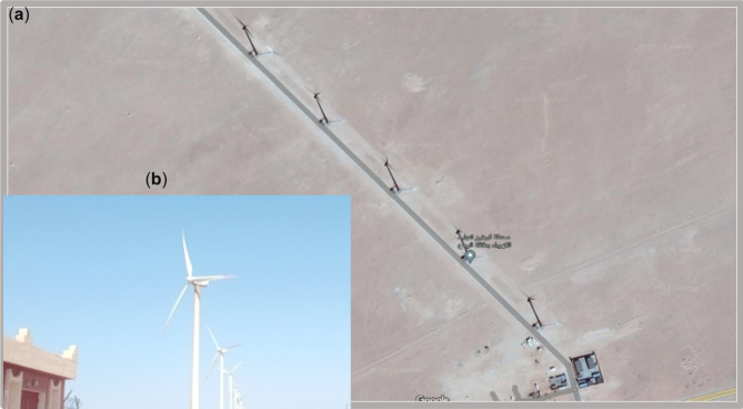
One such wind farm is Kabertene, the first in southern Algeria. Kabertene covers 30 ha of desert, 73 km north of Adrar, and was commissioned in 2014 with a nominal capacity of 10 MW (~ 10,200 kW). The onshore wind farm is owned by Shariket Kahraba wa Taket Moutadjadida (SKTM) and is operated by Sonelgaz. It consists of 12 GAMESA G52/850 wind turbines. With 55-meter-high towers and a rotor diameter of 52 m, the 850 kW turbines take advantage of the region’s strong winds, with an average of 8.5 m per second. The park feeds 10 (MWs) of nominal power into the grid. The 12 turbines are arranged directly according to the prevailing wind direction (Fig. 1). The Kabertene wind farm is connected to the electricity grid via its substation, which shows that Adrar can utilize its abundant wind resources.

Fig. 1.

Desert wind farm station investigated in this study: (a) aerial view and (b) ground view of the wind farm. The map was generated using Google Maps (Version 11, URL: https://maps.google.com).

The Kaberten wind farm currently supplies 10 megawatts (MWs) of rated power to the country. The horizontally aligned GAMESA G52/850 KW wind turbine had three blades with a rotor diameter of 52 m. The technical data of the wind turbine are listed in Table 1. 

Table 1.

Specifications of the wind turbines used at the desert wind farm station.

Wind turbine model: G52/850 | Manufacturer: Gamesa (Spain)
Normal power: 850 kW
Tower
Height	55 m
Base wall thickness	18 mm
Top wall thickness	10 mm
Rotor (blades & hub)
Number of blades	3
Rotor diameter	52 m
Rotor speed	14.6–30.8 rpm
Swept area	2,124 m2
Blade length	25.3 m
Wind speeds
Cut-in wind speed	4 m/s
Rated wind speed	16 m/s
Cutoff wind speed	25 m/s
Survival static wind speed	70 m/s
Weights
Nacelle	23 ton
Tower	62 ton
Rotor þ hub	10 ton
Total	80 ton

Methodology

Long short-term memory (LSTM)

Long short-term memory networks (LSTMs) are recurrent neural networks that are well suited for modeling sequential data. LSTMs were introduced in 1997 by Hochreiter and Schmidhuber^23, who solved the vanishing gradient problem of standard RNNs through gating mechanisms. The LSTM has a memory cell and three gates: an input gate, a forget gate, and an output gate^24,25. Depending on their importance, these gates allow the network to store or forget information in the cell state selectively²⁶. The sigmoidal gates output values between 0 and 1, which means “forget al.l” or “remember all " LSTMs use tangential functions to avoid gradient problems. Equations (6) and (10) illustrate the operations of the LSTM layers.

1

2

3

4

5

Here, is the input at time is the hidden state from the previous time step, and denotes the convolution operation. The gates and are the input, forget, and output gates, respectively, and is the cell state. The weight matrices and biases are learnable parameters that are optimized during training. The elementwise multiplication is denoted by , where represents the sigmoid activation function.

ConvLSTM Model

The LSTM architecture can be further enhanced by introducing a more sophisticated model that integrates both convolutional and recurrent neural networks. The Convolutional Long Short-Term Memory (ConvLSTM) model is a powerful extension of the standard LSTM architecture specifically designed for processing spatiotemporal data. This model combines the strengths of convolutional neural networks (CNNs) and long short-term memory (LSTM) networks to capture spatial and temporal dependencies effectively. ConvLSTM has already been successfully applied in various fields, such as predicting precipitation²⁷, recognizing violent videos²⁸, and predicting traffic flows²⁹. The ConvLSTM cell is essentially an LSTM cell with convolutional operations in the transitions from input to state and from state to state, replacing the fully connected operations in a traditional LSTM. The ConvLSTM equations can be represented as follows³⁰:

6

7

8

9

10

where ‘’ represents the Hadamard product and where represents the hidden and cell states at time .

Integrating the attention mechanism

The integration of the attention mechanism into recurrent neural networks, particularly long short-term memory (LSTM) networks, has significantly advanced the field of sequence modeling. Despite their effectiveness in addressing long-range dependencies in sequential data, conventional LSTM models have the limitation that they compress all information into a fixed-length vector, which can lead to the loss of important information. The attention mechanism solves this problem by allowing the model to focus on different parts of the input sequence with different degrees of importance. This method was first proposed by Bahdanau et al. (2014)³¹ to improve machine translation models and has since been widely adopted and refined in various applications, including speech recognition³², image captioning, and text summarization³³. Using a dynamic weighting approach, attention mechanisms have been shown to improve model performance by effectively managing the information of the input sequence^34,35.

In the context of an LSTM network, the attention mechanism can be integrated to enable the model to focus on relevant parts of the input sequence dynamically. The core idea is to map a query and set of key-value pairs to an output, where the query, keys, values, and output are all vectors. The output is computed as the weighted sum of the values, where the weights are determined by a compatibility function that measures the relevance of the keys to the query. The first step involves mapping the input sequence to a hidden state :

11

where is a nonlinear activation function and where represents the hidden state at time , with being the size of the hidden state.

For a given feature sequence , the attention score is computed using the previous hidden state and the cell state of the LSTM unit. Next, an attention mechanism is built through a stochastic attention model.

12

where is a vector and where and are matrices that are learnable parameters of the model. The vector has a length of , and each element measures the importance of the corresponding input feature sequence at time . These scores are then normalized via the Softmax function to produce the attention weights :

13

The attention weights indicate the degree of importance assigned to each feature sequence. The output of the attention model at time , denoted as the weighted input feature , is computed as:

14

This weighted sum replaces the original input in the LSTM equations, allowing the model to focus on the most relevant parts of the input sequence at each time step.

Hyperparameter grid search for optimal performance

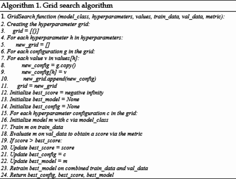
Machine learning requires hyperparameter optimization to determine the optimal parameters for model performance. A grid search, which systematically optimizes a predetermined collection of hyperparameters, is a popular tuning approach. This exhaustive strategy covers the search space but demands considerable computer power³⁶. Grid search improves model accuracy and generalizability in classification and regression³⁷. Method 2 details grid search Algorithm 1.

Model framework

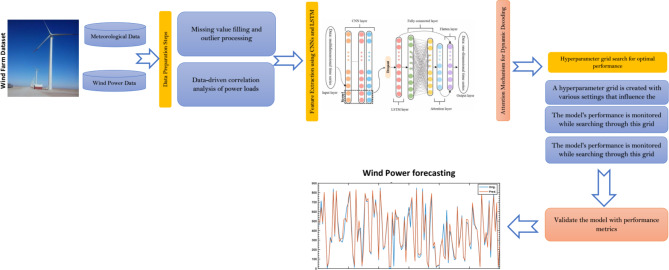
This section describes the Conv-DA-LSTM model development process in detail. Attention mechanisms and grid search hyperparameter optimization are included in the model. This development approach uses Python and deep learning frameworks such as TensorFlow and PyTorch for model generation and training. A powerful supercomputing infrastructure aids efficient calculations. The Conv Dual-Layer Long Short-Term Memory (ConvDL-LSTM) architecture and seamless attention integration (see Fig. 2) are described below:

Fig. 2.

Framework of this study.

• Step 1: Data are extracted and preprocessed from the data space by the data preparation module. We then use data to analyze the relationships between wind power and the influencing variables. Second, the module screens affect variables via the factors in Sect. 3.7. Historical wind power and influencing factor data are fed into the forecast model.

• Step 2: Convolutional neural networks collect complex input sequence patterns and characteristics. These CNN layers convolve input data to extract spatial characteristics and enhance the model’s local pattern awareness. Second, the CNN layers are followed by dual-layer LSTM units. Two LSTM layers are stacked in the dual-layer LSTM design to capture sequential dependencies better.

• Step 3: The attention mechanism weighs the input-sequence components during dynamic decoding.

• Step 4: A hyperparameter grid with the model affecting hyperparameters is produced. The model’s performance is monitored while searching for the grid, and the hyperparameter configuration with the best validation results is chosen.

• Step 5: Performance measures, including the RMSE, MAE, and RRMSE, are used to evaluate the final Conv-DA-LSTM model against an independent test set.

In summary, this section describes a complete approach for developing and evaluating an advanced deep-learning model for sequential data processing. The integration of attention mechanisms and convolutional and recurrent neural networks, along with hyperparameter optimization, forms a robust framework capable of capturing intricate spatiotemporal relationships. The evaluation metrics enable us to gauge the model’s effectiveness in real-world applications.

Evaluation metrics

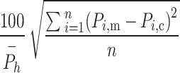
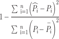
The accuracy of the models was evaluated via several criteria, as summarized in Table 6. The metrics include (total observations), (measured value), (estimated value), and (mean value of the measured values)^38–40. The root mean square error (RMSE) measures the difference between the predicted and observed values and enables a comparison of the errors between the models. The root mean absolute error (MAE) indicates the closeness of the estimated values to the experimental data. The root relative squared error (RRMSE) divides the RMSE by the true mean; a lower RRMSE indicates a better model. The correlation coefficient (R²), which lies between 0 and 1, indicates the quality of the linear relationship between the estimated and measured values^41–45 Table 2.

Table 6.

The monthly root mean square relative error (RRMSE) for the classical machine learning models.

Model	JAN	FEB	MAR	APR	MAY	JUN	JUL	AUG	SEP	OCT	NOV	DEC
MLP	36.286	32.22	29.574	30.183	27.547	21.52	22.986	28.405	38.711	36.732	52.994	31.102
LNR	27.631	26.933	25.039	28.537	23.115	20.464	19.186	24.439	28.079	29.453	24.055	15.156
SVR	47.115	58.371	56.553	66.541	59.342	56.505	40.599	52.006	67.752	75.981	69.147	37.137
DTR	24.658	26.303	25.968	31.114	26.759	21.908	23.215	27.316	30.123	32.395	17.809	14.120
RCV	27.631	26.932	25.039	28.536	23.115	20.463	19.186	24.439	28.084	29.453	24.055	15.156
ENet	28.291	27.371	25.743	28.796	23.639	20.781	19.482	24.621	28.876	30.372	24.823	15.881
LCV	27.618	26.932	25.041	28.535	23.114	20.456	19.185	24.436	28.085	29.459	24.054	15.152

Table 2.

Metrics used for performance evaluation.

Evaluation metric	Abbreviation	Formula	#Eq.
Mean absolute error			(15)
Root mean square error			(16)
Relative RMSE			(17)
Correlation coefficient	2		(18)

Results

Data collection and analysis

This subsection describes the data collection process and the exploratory analysis of the dataset. The data were collected from December 2018 to November 2019 at a desert wind farm, with measurements recorded every half hour. The process started with the gathering of raw data from the wind farm’s sensors and instruments. After that, a thorough descriptive statistical analysis was performed to understand the distribution and characteristics of each variable in the dataset. The results of this descriptive analysis are summarized in Table 3. The data show remarkable diversity in the temperature (TEM) data, highlighted by a standard deviation of 9.46 and a wide range of 1.33–46.05. The temperature distribution is slightly negative (-0.16), with a concentration of values at the upper end. In contrast, the wind speed (SPD) data show comparatively less variability, highlighted by a standard deviation of 2.53 and a smaller range of 16.68. The distribution of the wind speed is approximately normal.

Table 3.

Summary statistics for temperature, wind speed, and power output variables.

Stat.	TEM	SPD	POW
Mean	26.10	7.61	378.68
Median	26.84	7.79	339.17
Mode	37.03	10.05	849.63
Standard Deviation	9.46	2.53	271.72
Sample Variance	89.54	6.41	73831.78
Kurtosis	-0.92	-0.73	-1.27
Skewness	-0.16	-0.08	0.27
Range	44.73	16.68	883.19
Minimum	1.33	0.80	0.01
Maximum	46.0593	17.4793	883.2

The power output (POW) data show the most variability, with a high standard deviation of 271.72 and a range of 883.19. The median power output is 339.17, and the mean is 378.68, showing that some extremely high values pull the mean above the median. This is confirmed by the positive skewness (0.27) and a mode (849.63) that is much greater than the median. The data show that power generation in this desert environment is highly variable and depends on temperature and wind speed, which also show significant fluctuations.

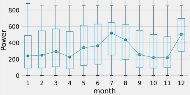
Figure 3 shows the monthly distribution of half-hourly wind power, measured in kilowatts (kW). Wind power peaks in winter (January and February) and decreases in summer (July and August). This is consistent with the trend that wind speeds are higher in winter than in summer. The figure also shows outliers in the data; for example, January is above average at 800 kW. Outliers can be due to storms, high pressure, or shifts in the direction of the wind.

Fig. 3.

Distribution of half-hourly wind power according to month.

Table 4 divides the wind speeds into weak, medium, and strong winds. The figure also shows the percentage of each category, the cumulative percentage, and the average daily wind speed. The category of weak winds from 0 to 8.99 m/s accounts for 65.04% of the total data. The cumulative percentage shows that weak winds account for 65.04% of the observations. The average daily wind speed for weak winds is 6.15 m/s.

Table 4.

Wind speed categorization and distribution.

Class	Categories	Speed range (m/S)	Percentage (%)	Cumulative percentage (%)	Average daily wind speed (m/s)
1	Weak Wind	0–8.99	65.04	65.04	6.15
2	Medium Wind	9–12.99	34.08	99.12	10.22
3	high Wind	13–25	0.88	100	14.02

Medium winds of 9–12.99 m/s account for 34.08% of the data. If the proportion of weak winds is added, the result is that the medium winds cumulatively account for 99.12% of the total observations. The average speed is 10.22 m/s for medium winds. Finally, strong winds of 13–25 m/s account for only 0.88% of the data. Together with the other categories, strong winds cumulatively account for 100% of the observations. The average daily wind speed for strong winds is 14.02 m/s.

Table 5 shows the overall results of the ANOVA used to analyze the factors that influence wind energy. For the factor month, the F value of 58.60 and extremely low P value of 3.15E–129 illustrate the significant influence of the months on the dataset. These values indicate that the month strongly influences the variance of the data.

Table 5.

Overall ANOVA statistical insights into the factors influencing the dataset.

Source	DF	Sum of Squares	Mean Square	F Value	P Value
Month	11	1.42E + 07	1,288,014	58.60	3.15E-129
SPD Class	2	1.05E + 09	5.26E + 08	23928.78	0
Model	13	1.17E + 09	9.00E + 07	4096.11	0
Error	22,551	4.96E + 08	21977.96	-	-
Corrected Total	22,564	1.67E + 09	-	-	-

The SPD class is even more convincing, with a P value of 0 and an F value of 23928.78, which underlines a highly significant influence. The variance captured here is substantial. The model’s P value of 0 and F value of 4096.11 effectively explain the variance in wind energy. In the error range, the mean square value (21977.96) highlights the variability that the model does not explain. This is to be expected, given the complexity of wind energy forecasting.

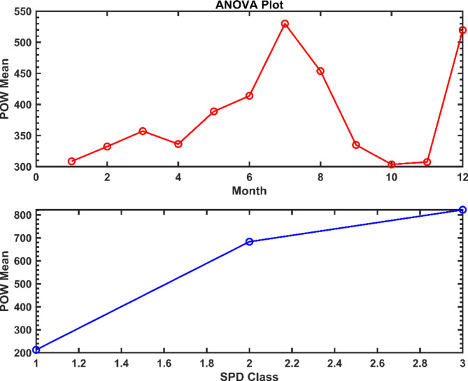
Figure 4 shows ANOVA plots comparing the first factor (month) with the POW mean and the second factor B (SPD class) with the POW mean. The monthly plot shows that wind power is highest in July at 529 kW and lowest in October/November at 304 kW. This finding is consistent with Table 4, which shows a highly significant monthly effect. The plot of the wind speed classes shows that higher classes have a much higher mean power. The wind speed class plot clearly shows an increase in the mean power output with increasing wind speed, with class 3’s mean power being more than three times greater than that of class 1.

Fig. 4.

ANOVA Plots: Month vs. POW Mean and Class SPD vs. POW Mean.

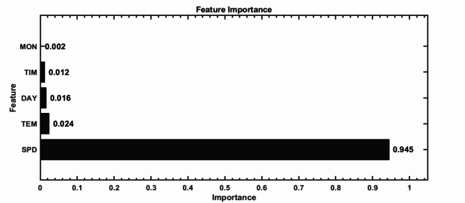
In Fig. 5, the graph shows the relative importance of features from the random forest model. Speed (SPD) is the most influential factor, with a remarkably high value of 0.945. This high importance of SPD indicates its dominant role in the analyzed context. The temperature (TEM) is followed by a much lower importance of 0.024, indicating a comparatively low influence on the outcome.

Fig. 5.

Key feature importance rankings.

The importance of Day (DAY) is 0.016. Although it is less influential than SPD, DAY still contributes to the overall understanding of the dataset. Time (TIM) has a slightly lower importance of 0.012, indicating a relatively small influence on the results. Finally, the month (MON) has the lowest importance among the analyzed features, with a value of 0.002. This result implies that MONs have a marginal influence on the analyzed system or phenomenon.

Given the results of Fig. 5, speed (SPD) occupies a key position in terms of feature importance, vastly outweighing all other features. Temperature (TEM) is the second most important feature, but its importance is much closer to that of the DAY and TIM than to that of the SPD. Thus, while SPD is crucial for accurate predictions and model evaluation, considering other features, such as TEM, DAY, and TIM, may offer marginal improvements depending on the model’s requirements.

Analyzing the impact of model optimization

This section presents a comparative assessment of traditional machine learning and deep learning models for wind energy forecasting. The performance indicators for each modeling approach were tested under various scenarios. First, we analyzed the monthly performance of traditional machine learning models. Table 6 summarizes the classical models’ relative root-mean-square error (RRMSE) values by month. RRMSE values indicate prediction accuracy, with lower values suggesting better forecasts. The multilayer perceptron (MLP) model had the largest error, peaking at 52.994 in November. June has the lowest error of 21.52. The linear regression model (LNR) fared better, with January errors of 27.631 and December errors of 15.156.

The monthly performance variation was the largest for the support vector regression (SVR) model. Its inaccuracy varied from 75.981 in October to 37.137 in December. The decision tree regression (DTR) model was more constant, peaking at 32.395 in October and decreasing to 14.12 in December. Elastic net regression, ridge regression, and LASSO regression with cross-validation (LCV) performed similarly. The summer errors were less than 20, whereas the autumn errors were above 30. These monthly data challenge the MLP model the most, whereas the LNR and tree-based models perform better.

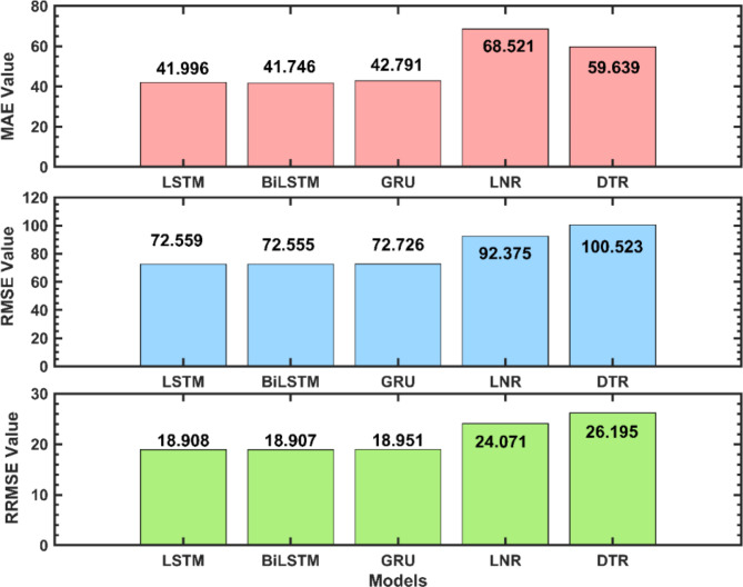
Next, the performance of deep learning models versus classical machine learning techniques was examined. Figure 6 compares these models via three error metrics: MAE, RMSE, and RRMSE. The deep learning models evaluated are the LSTM, the BiLSTM, and the GRU. The LSTM and BiLSTM models performed very similarly, with almost identical MAE, RMSE, and RRMSE values of 41–42, 72, and 18.9, respectively. This suggests that the bidirectional capability of the BiLSTM did not significantly improve performance over that of the standard LSTM on this task.

Fig. 6.

Performance comparison of selected deep learning and best-classical models.

In contrast, the GRU model performed slightly worse than both the LSTM and BiLSTM models did, with higher errors of 42 MAEs, 72 RMSEs, and 18.95 RRMSEs. Nevertheless, all three deep learning models outperformed the classic LNR and DTR models. For example, the LNR model had errors of 68 MAEs, 92 RMSEs, and 24 RRMSEs, whereas the decision tree model performed even worse, with errors of 59 MAEs, 100 RMSEs, and 26 RRMSEs. These results highlight the superior ability of deep learning models to model nonlinear relationships, thereby improving prediction performance compared with the linear LNR and tree-based DTR models.

To further improve our models, we explored the impact of hyperparameter optimization on the LSTM and ConvLSTM architectures. Table 7 compares the optimized hyperparameters for the Conv-DA-LSTM-GSA and LSTM models. A larger stack size of 32 was used for Conv-DA-LSTM-GSA than 16 for LSTM. More epochs were also required to optimize Conv-DA-LSTM − 200 versus 150 epochs for LSTM. Both models use the Adam optimizer for gradient descent optimization. The LSTM uses a dropout rate of 0.3 for regularization. The Conv-DA-LSTM-GSA had a kernel size of 2 and 128 filters to recognize spatial patterns. Conv-DA-LSTM-GSA requires 70 hidden units, whereas LSTM requires 50, with LSTM using tanh activation between layers, unlike Conv-DA-LSTM-GSA. Consequently, the optimized hyperparameters led to notable performance gains, as shown in Table 8. Specifically, for the LSTM models, optimization resulted in a reduction in the MAE by 7.80%, the RMSE by 4.24%, and the RRMSE by 4.24% compared with the nonoptimized LSTM. Additionally, the R² value improved by approximately 0.65%. These improvements emphasize the importance of fine-tuning, demonstrating the potential for optimized models to enhance predictive accuracy substantially.

Table 7.

Tuned hyperparameters of the optimized Conv-DA-LSTM and LSTM models.

Conv-DA-LSTM-GSA	Value	LSTM	Value
Batch size	32	Batch Size	16
Epochs	200	Epochs	150
Optimizer	adam	Optimizer	adam
Kerne size	2	Dropout Rate	0.3
Filters	128	Activation	tanh
Hidde Units	70	Hidden Units	50

Table 8.

Evaluating the optimization effects on LSTM and ConvLSTM.

Model Name	MAE[MW]	RMSE[MW]	RRMSE[%]	R2[-]
LSTM	0.0455	0.0758	19.746	0.922
LSTM-GSA	0.0420	0.0726	18.908	0.928
Conv-DA-LSTM	0.0433	0.0726	18.910	0.928
Conv-DA-LSTM-GSA	0.0417	0.0719	18.727	0.930

For the Conv-DA-LSTM models, the nonoptimized version performs better than the nonoptimized LSTM, with a lower MAE of 0.0433, RMSE of 0.0726, and RRMSE of 18.910. After optimization, the Conv-DA-LSTM-GSA model performs best overall, with the lowest MAE of 0.0417, an RMSE of 0.0719, an RRMSE of 18.727, and the highest R² of 0.93. In addition, optimization of the Conv-DA-LSTM model results in a 3.70% lower MAE, a 0.97% lower RMSE, and a 0.97% lower RRMSE than those of the nonoptimized version. The R² metric increases by approximately 0.22% after optimization.

To put these improvements into perspective, consider a large wind farm with a capacity of 100 MW. A 3.70% reduction in the MAE could indicate a difference between accurately predicting a 50 MW output and a 51.85 MW output. This improved accuracy could significantly enhance grid integration and energy trading strategies.

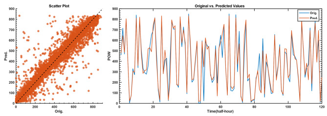
The effectiveness of the optimized Conv-DA-LSTM model can be seen visually in Fig. 7. The original wind power values are shown in blue, while the predicted values are shown in red. Overall, the figure shows a close match between the predicted and original wind speed values, confirming the accuracy of the model and its high potential for reliable wind speed predictions.

Fig. 7.

Comparison of the original and predicted wind power values.

Generally, the optimization of both the LSTM and Conv-DA-LSTM architectures leads to significant improvements over the nonoptimized versions, with gains of 4–8% for the most important metrics. The optimized Conv-DA-LSTM-GSA model performs best in terms of all the error and accuracy metrics.

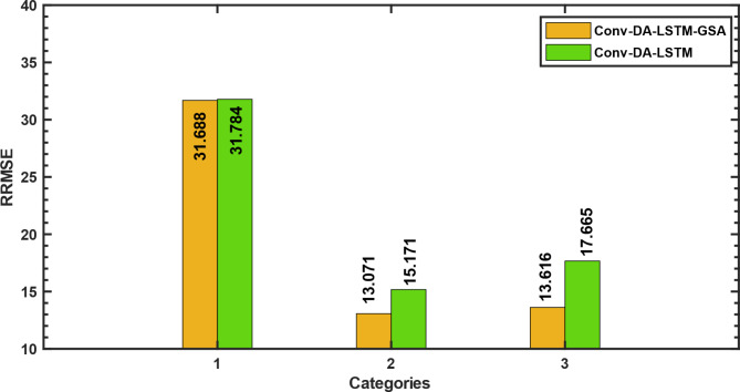
Furthermore, the effects of optimization on the Conv-DA-LSTM model for different wind speed categories were analyzed. Figure 8 compares the RRMSE of the wind speed category of Conv-DA-LSTM with and without optimization. In category 1 (low wind range), the Conv-DA-LSTM-GSA has an RRMSE of 31.688, whereas the nonoptimized version (Conv-DA-LSTM) has an RRMSE of 31.784, showing a 0.3% improvement. In category 2 (moderate wind range), the Conv-DA-LSTM-GSA achieves an RRMSE of 13.071, in contrast to the Conv-DA-LSTM model’s RRMSE of 15.171, which is a reduction of 13.9%. In category 3 (the strong wind range), the Conv-DA-LSTM-GSA achieves an RRMSE of 13.616, whereas the Conv-DA-LSTM model’s RRMSE is 17.665, indicating an improvement of 22.9%. For all the wind speed categories, the optimized Conv-DA-LSTM model consistently outperforms the Conv-DA-LSTM model. The improvements range from 0.3% under low winds to 22.9% under high winds. These results highlight the advantages of optimization, especially at relatively high wind speeds, which are characterized by complicated dynamics.

Fig. 8.

Evaluating the impact of optimization on Conv-DA-LSTM by wind speed categories.

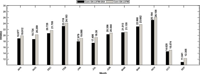
Additionally, the effects of optimization on the Conv-DA-LSTM model in different months of the year were examined. Figure 9 shows a comprehensive analysis of the monthly root mean square error (RMSE) values of the Conv-DA-LSTM model and compares its performance with and without optimization. In January, the Conv-DA-LSTM-GSA model had an RRMSE of 18.977, whereas the Conv-DA-LSTM model’s RRMSE was 19.912, a remarkable improvement of 4.7%. Similar RRMSE reductions due to optimization are observed in February (4.6%), March (4.5%), April (4.3%), and May (6.2%). In the summer months, from June to August, the improvements are between 1.6% and 2.3%. Significant improvements were also recorded in September (3%) and October (3.5%). November presented an increase of 3%, whereas December presented the greatest optimization increase, with a 10.2% lower RRMSE. In all months, the optimized version of Conv-DA-LSTM outperforms the nonoptimized version, with RRMSE reductions ranging from 1.6 to 10.2%. The improvements are evident every month and highlight the benefits of model optimization. These monthly enhancements underscore the consistency and robustness of the optimized deep learning approach, particularly when contrasted with the variable performance of classical models throughout the year, as shown in Table 7.

Fig. 9.

Comparing the monthly RRMSE of Conv-DA-LSTM with and without optimization.

Finally, to contextualize our model’s performance within the broader field of wind power forecasting, we compared our results with those from recent literature. As presented in Table 9, our proposed model, which was applied to wind power forecasting in southern Algeria, achieved an R² of 0.93 and an RMSE of 0.0719 MW. This indicates a more accurate predictive capability relative to the other models listed. For example, the RMSE of the proposed model is lower than that of the WNN model by Guo et al. (2022)⁴⁷ and the EEMD-LSSVM model by Jiang and Huang (2017)⁵⁰, which had RMSEs of 0.078 and 0.075, respectively. Moreover, the R² value of the proposed model is 0.93 greater than the R² values of the WPCA-PSO-GRU model by Xiao et al. (2023)⁴⁶ and the PSO-LSTM model by Jiang and Liu (2023)⁴⁸, which both reported R² values of 0.917 and 0.92. This suggests that the proposed model not only reduces prediction errors but also explains a greater proportion of variance, thereby enhancing overall model accuracy and reliability. However, it is important to acknowledge that further validation across different datasets and locations would be beneficial to fully establish the model’s generalizability.

Table 9.

Performance comparison of the proposed model with existing methods in the literature.

Author & Ref.	Model used	Location	RMSE [MW]	R² or R [-]
Xiao et al., 202346	WPCA-PSO-GRU	Northwest China	2.22	0.917
Guo et al., 202247	WNN	China	0.078	0.92
Jiang and Liu, 202348	PSO-LSTM	China	0.13833	0.92
Jiang et al., 202049	TVF-EMD	China	0.4119	-
Jiang and Huang, 201750	EEMD-LSSVM	USA	0.075	-
This study	Proposed model	Algeria’s South	0.0719	0.93

In summary, our analysis confirms the superiority of deep learning models in wind energy forecasting, with our optimized Conv-DA-LSTM-GSA model proving particularly effective. The model consistently shows improvements across various wind speed categories and throughout different months, highlighting its robustness and reliability. Moreover, a comparison with the literature demonstrates the significant advancements our model has made in the field. These findings validate our methodology and pave the way for more accurate and dependable wind energy predictions, which are crucial for the efficient integration of wind power into modern energy systems.

Discussion

The results and comparisons suggest that deep learning models such as LSTM and ConvLSTM have the potential to increase wind power prediction accuracy compared with traditional machine learning approaches. The deep learning models were able to capture better the nonlinear interactions in the data that impact the wind power output.

The LSTM and BiLSTM models performed very similarly, suggesting that the bidirectional capability did not significantly improve performance on this task. The GRU model performed slightly worse than the LSTM and BiLSTM models did, showing differences between the deep learning architectures⁵¹. However, all the deep learning models significantly outperformed the classical linear regression and decision tree regression models in terms of error metrics such as the MAE, RMSE, and RRMSE. This aligns with previous research showing that deep learning models perform better than classical techniques do in wind power forecasting^52,53.

Hyperparameter tuning and optimization further improved the LSTM and Conv-DA-LSTM models. For the LSTM, the optimization reduced the errors by 4–8% and increased the accuracy (R2) by 0.65% compared with the nonoptimized version. Compared with Conv-DA-LSTM-LSTM, the Conv-DA-LSTM-GSA achieves the best overall performance, reducing the number of errors by 1–4% and increasing the accuracy (R²) by 0.22%. The use of attention mechanisms likely helped the model focus on the most relevant input features⁵⁴.

The Conv-DA-LSTM-GSA model analysis revealed the largest gains at higher wind speeds, with an error reduction of up to 22.9% under strong winds. This highlights the benefits of optimization, especially in complex wind dynamics. In terms of monthly performance, the Conv-DA-LSTM-GSA reduced the number of errors by 1.6–10.2% in all months, confirming the consistent effect of optimization.

In the broader context of wind power forecasting research, our optimized Conv-DA-LSTM-GSA model achieved competitive results, with an R² of 0.93, outperforming several recent studies in different geographical locations. This suggests strong potential for the model’s applicability across diverse contexts, although further validation with various datasets would be beneficial to establish its generalizability fully.

While hybrid deep learning approaches, particularly optimized ConvLSTM models, have demonstrated significant improvements in wind power forecasting accuracy, it is important to acknowledge the advancements of SOTA models such as transformers. These models outperform traditional RNN models in various time series prediction tasks and could offer further enhancements in wind power forecasting.

In summary, the results indicate that, compared with classical machine learning, hybrid deep learning approaches can significantly improve the accuracy of wind power forecasts. However, challenges remain in the application of these complex models, including computational cost and interpretability⁵⁵. Further research on network optimization could make deep learning more feasible for real-world wind power forecasting.

Conclusions

This work developed and evaluated an optimized hybrid deep learning technique for desert short-term wind energy prediction to improve accuracy and dependability. Meteorological data, including wind speed and temperature, were used to analyze the complicated climatic linkages impacting wind energy generation.

Preprocessed Adrar wind farm data were used to enhance model inputs via feature engineering. Advanced deep learning architectures and traditional machine learning models were compared. The performance and wind speeds were measured over several months. The research also examined how hyperparameter optimization for the LSTM and Conv-DA-LSTM models affected the prediction accuracy.

The results revealed that deep learning models consistently outperformed classical machine learning techniques in wind energy forecasting. Among classical models, linear regression and decision trees demonstrated more robust performance across different months, whereas support vector regression exhibited the highest variability. The MLP model struggled the most with monthly data variations. In the comparison of deep learning architectures, the LSTM and BiLSTM models performed similarly, with the GRU model showing slightly lower accuracy. All three deep learning models significantly outperform the best classical techniques, highlighting their superior ability to capture nonlinear relationships in wind energy data.

Hyperparameter optimization had a substantial effect, particularly for the Conv-DA-LSTM model. The Conv-DA-LSTM-GSA achieved the best overall performance, with the lowest error rates (MAE: 41.730, RMSE: 71.866, RRMSE: 18.727) and highest accuracy (R²: 0.930). Compared with the nonoptimized version, optimization resulted in improvements of 3.64% in the MAE, 0.97% in the RMSE, and 0.97% in the RRMSE.

The performance analysis across wind speed categories indicated that the optimization benefits were most pronounced for higher wind speeds, with improvements ranging from 0.3% for low winds to 22.9% for high winds, suggesting effective capture of dynamics under strong wind conditions. Monthly analysis revealed that Conv-DA-LSTM-GSA consistently outperformed its nonoptimized counterpart throughout the year, with RRMSE reductions ranging from 1.6 to 10.2%. The most significant improvements were observed in the winter months, especially December, indicating enhanced model performance in handling seasonal variations.

In a nutshell, this work demonstrates the superior performance of optimized hybrid deep learning models, particularly the Conv-DA-LSTM-GSA architecture, for short-term wind energy forecasting in desert environments. The integration of meteorological data and advanced optimization techniques significantly enhances the prediction accuracy across various wind speed ranges and seasonal conditions. Potential future research avenues may include the incorporation of additional meteorological and geographical data, investigating transfer learning for adapting models to different wind farm locations, and developing ensemble methods that combine multiple deep learning architectures.

Author contributions

Conceptualization, M.B; N.B; K.B; M.G; methodology and software validation M.A; M.B; B.Z; A.H.A; E.M.E; formal analysis and writing—original draft, A.H.A, K.B; B.Z; A.K ; M.B, D.S.K, M.E; M.G; writing—review and editing, N.B; M.E, A.K; A.H.A.; visualization, M.E ; N.B, and D.S.K. All authors have read and agreed to the published version of the manuscript.

Data availability

The authors confirm that the data supporting the findings of this study are available within the article.

Declarations

Competing interests

The authors declare that they have no known competing financial interests or personal relationships that could have appeared to influence the work reported in this paper.

References

- 1.Power to Gas for Future Renewable based Energy Systems. IET Renew. Power Gener; 14:3281–3283. 10.1049/iet-rpg.2021.0002. (2020). [Google Scholar]
- 2.Henner, D. REN21. Ren21 - GLOBAL STATUS REPORT. (2017).
- 3.Edenhofer, O. & Seyboth, K. Intergovernmental Panel on Climate Change (IPCC). Encycl. Energy, Nat. Resour. Environ. Econ., vol. 1–3, (2013). 10.1016/B978-0-12-375067-9.00128-5
- 4.EL-Shimy, M. et al. Economics of Variable Renewable Sources for Electric Power Production (2017).
- 5.Himri, Y., Rehman, S., Draoui, B. & Himri, S. Wind power potential assessment for three locations in Algeria. Renew. Sustain. Energy Rev.12, 2495–2504. 10.1016/j.rser.2007.06.007 (2008). [Google Scholar]
- 6.IRENA greeted as milestone for renewables. Renew. Energy Focus; 9:19. 10.1016/s1755-0084(09)70029-8. (2009). [Google Scholar]
- 7.Giebel, G. & Kariniotakis, G. Wind power forecasting-a review of the state of the art. Renew. Energy Forecast. Model. Appl.10.1016/B978-0-08-100504-0.00003-2 (2017). [Google Scholar]
- 8.Tawn, R. & Browell, J. A review of very short-term wind and solar power forecasting. Renew. Sustain. Energy Rev.153, 111758. 10.1016/j.rser.2021.111758 (2022). [Google Scholar]
- 9.Wang, J., Song, Y., Liu, F. & Hou, R. Analysis and application of forecasting models in wind power integration: a review of multi-step-ahead wind speed forecasting models. Renew. Sustain. Energy Rev.60, 960–981. 10.1016/j.rser.2016.01.114 (2016). [Google Scholar]
- 10.Zhang, Y., Chen, B., Pan, G. & Zhao, Y. A novel hybrid model based on VMD-WT and PCA-BP-RBF neural network for short-term wind speed forecasting. Energy Convers. Manag. 195, 180–197. 10.1016/j.enconman.2019.05.005 (2019). [Google Scholar]
- 11.Chen, J. et al. Wind speed forecasting using nonlinear-learning ensemble of deep learning time series prediction and extremal optimization. Energy Convers. Manag 2018;165. 10.1016/j.enconman.2018.03.098
- 12.He, Q., Wang, J. & Lu, H. A hybrid system for short-term wind speed forecasting. Appl. Energy. 226, 756–771. 10.1016/j.apenergy.2018.06.053 (2018). [Google Scholar]
- 13.Wang, J-Z., Wang, Y. & Jiang, P. The study and application of a novel hybrid forecasting model – a case study of wind speed forecasting in China. Appl. Energy. 143, 472–488. 10.1016/j.apenergy.2015.01.038 (2015). [Google Scholar]
- 14.Liu, H., Mi, X. & Li, Y. Wind speed forecasting method based on deep learning strategy using empirical wavelet transform, long short term memory neural network and Elman neural network. Energy Convers. Manag. 156, 498–514. 10.1016/j.enconman.2017.11.053 (2018). [Google Scholar]
- 15.Hossain, M. A., Chakrabortty, R. K., Elsawah, S. & Ryan, M. J. Very short-term forecasting of wind power generation using hybrid deep learning model. J. Clean. Prod.296, 126564. 10.1016/j.jclepro.2021.126564 (2021). [Google Scholar]
- 16.Wu, Q., Guan, F., Lv, C. & Huang, Y. Ultra-short‐term multi‐step wind power forecasting based on CNN‐LSTM. IET Renew. Power Gener. 15, 1019–1029. 10.1049/rpg2.12085 (2021). [Google Scholar]
- 17.Neshat, M., Majidi Nezhad, M., Mirjalili, S., Piras, G. & Garcia, D. A. Quaternion convolutional long short-term memory neural model with an adaptive decomposition method for wind speed forecasting: north aegean islands case studies. Energy Convers. Manag. 259, 115590. 10.1016/j.enconman.2022.115590 (2022). [Google Scholar]
- 18.Nguyen, T. H. T., Van Pham, N., Nguyen, V. N. N., Pham, H. M. & Phan, Q. B. Forecasting wind speed using a hybrid model of convolutional neural network and long-short term memory with Boruta Algorithm-based feature selection. J. Appl. Sci. Eng.26, 1053–1060 (2022). [Google Scholar]
- 19.Ai, X., Li, S. & Xu, H. Short-term wind speed forecasting based on two-stage preprocessing method, sparrow search algorithm and long short-term memory neural network. Energy Rep.8, 14997–15010. 10.1016/j.egyr.2022.11.051 (2022). [Google Scholar]
- 20.Gensler, A., Henze, J., Sick, B., Raabe, N. & LSTM Neural Networks. Deep Learning for solar power forecasting - An approach using AutoEncoder and. IEEE Int. Conf. Syst. Man, Cybern. SMC 2016 - Conf. Proc., Institute of Electrical and Electronics Engineers Inc.; 2017, pp. 2858–65. (2016). 10.1109/SMC.2016.7844673
- 21.Hu, H., Wang, L. & Lv, S-X. Forecasting energy consumption and wind power generation using deep echo state network. Renew. Energy. 154, 598–613. 10.1016/j.renene.2020.03.042 (2020). [Google Scholar]
- 22.Diop, S., Traore, P. S., Ndiaye, M. L. & Wind Power Forecasting Using Machine Learning Algorithms. 9 th Int Renew Sustain Energy Conf 2021. (2021). 10.1109/irsec53969.2021.9741109
- 23.Hochreiter, S. & Schmidhuber, J. Long short-term memory. Neural Comput.9, 1735–1780. 10.1162/neco.1997.9.8.1735 (1997). [DOI] [PubMed] [Google Scholar]
- 24.Yadav, S. et al. State of the art in energy consumption using deep learning models. AIP Adv.14, 65306. 10.1063/5.0213366 (2024). [Google Scholar]
- 25.El-kenawy, E-S-M. et al. Global scale solar energy harnessing: an advanced intra-hourly diffuse solar irradiance predicting framework for solar energy projects. Neural Comput. Appl.10.1007/s00521-024-09608-y (2024). [Google Scholar]
- 26.Ahmed, A. et al. Global control of electrical supply: a variational mode decomposition-aided deep learning model for energy consumption prediction. Energy Rep. , 2152–2165 (2023).
- 27.Shi, X. et al. Convolutional LSTM network: a machine learning approach for precipitation nowcasting. Adv. Neural Inf. Process. Syst.28, 802–810 (2015). [Google Scholar]
- 28.Sudhakaran, S. & Lanz, O. Learning to detect violent videos using convolutional long short-term memory. 2017 14th IEEE Int. Conf. Adv. Video Signal. Based Surveill. IEEE, 1–6 (2017). [Google Scholar]
- 29.Yao, H. et al. Modeling spatial-temporal dynamics for traffic prediction. 1, (2018)
- 30.He, J., Yang, H., Zhou, S., Chen, J. & Chen, M. A dual-attention-mechanism Multi-channel Convolutional LSTM for short-term wind speed prediction. Atmos. (Basel). 14, 71 (2022). [Google Scholar]
- 31.Bahdanau, D., Cho, K. & Bengio, Y. Neural machine translation by jointly learning to align and translate. arXiv Prepr. arXiv1409.0473 (2014).
- 32.Chan, W., Jaitly, N., Le, Q. & Vinyals, O. Listen, attend and spell: a neural network for large vocabulary conversational speech recognition. 2016 IEEE International Conference on Acoustics, Speech and Signal Processing (ICASSP), pp. 4960–4964. 10.1109/ICASSP.2016.7472621 (Shanghai, China, 2016).
- 33.Cheng, J. & Lapata, M. Neural summarization by extracting sentences and words. arXiv preprintarXiv:1603.07252 10.48550/arXiv.1603.07252 (2016).
- 34.Luong, M-T., Pham, H. & Manning, C. D. Effective approaches to attention-based neural machine translation. arXiv Prepr. arXiv1508.04025 (2015). 10.48550/arXiv.1508.04025.
- 35.Vaswani, A. et al. Attention is all you need. Adv. Neural Inf. Process. Syst.30 6000–6010 (2017).
- 36.Belete, D. M. & Huchaiah, M. D. Grid search in hyperparameter optimization of machine learning models for prediction of HIV/AIDS test results. Int. J. Comput. Appl.44, 875–886 (2022). [Google Scholar]
- 37.Hsu, C-W., Chang, C-C. & Lin, C-J. A practical guide to support vector classification (2003).
- 38.Guermoui, M. et al. An analysis of case studies for advancing photovoltaic power forecasting through multi-scale fusion techniques. Sci. Rep.14, 6653 (2024). [DOI] [PMC free article] [PubMed] [Google Scholar]
- 39.Dahmani, A. et al. Assessing the Efficacy of Improved Learning in Hourly Global Irradiance Prediction (Comput Mater Contin, 2023).
- 40.Benatallah, M. et al. Solar Radiation Prediction in Adrar, Algeria: a Case Study of Hybrid Extreme Machine-based techniques. Int. J. Eng. Res. Afr.68, 151–164 (2024). [Google Scholar]
- 41.Djaafari, A. et al. Hourly predictions of direct normal irradiation using an innovative hybrid LSTM model for concentrating solar power projects in hyper-arid regions. Energy Rep.8, 15548–15562 (2022). [Google Scholar]
- 42.Hassan, M. A., Salem, H., Bailek, N. & Kisi, O. Random Forest Ensemble-Based Predictions of On-Road Vehicular Emissions and Fuel Consumption in Developing Urban Areas (Sustainability, 2023).
- 43.Yehia, M. H., Hassan, M. A., Abed, N., Khalil, A. & Bailek, N. Combined Thermal Performance Enhancement of Parabolic Trough Collectors Using Alumina Nanoparticles and Internal Fins. Int. J. Eng. Res. Africa, vol. 62, Trans Tech Publ; pp. 107–32. (2022).
- 44.Jamei, M. et al. Data-Driven models for Predicting Solar Radiation in semi-arid regions. Comput. Mater. Contin. 74, 1625–1640 (2023). [Google Scholar]
- 45.Guermoui, M., Bouchouicha, K., Benkaciali, S., Gairaa, K. & Bailek, N. New soft computing model for multi-hours forecasting of global solar radiation. Eur. Phys. J. Plus. 137, 162 (2022). [Google Scholar]
- 46.Xiao, Y., Zou, C., Chi, H. & Fang, R. Boosted GRU model for short-term forecasting of wind power with feature-weighted principal component analysis. Energy. 267, 126503 (2023). [Google Scholar]
- 47.Guo, N-Z. et al. A physics-inspired neural network model for short-term wind power prediction considering wake effects. Energy. 261, 125208. 10.1016/j.energy.2022.125208 (2022). [Google Scholar]
- 48.Jiang, T. & Liu, Y. A short-term wind power prediction approach based on ensemble empirical mode decomposition and improved long short-term memory. Comput. Electr. Eng.110, 108830. 10.1016/j.compeleceng.2023.108830 (2023). [Google Scholar]
- 49.Jiang, Y., Liu, S., Zhao, N., Xin, J. & Wu, B. Short-term wind speed prediction using time varying filter-based empirical mode decomposition and group method of data handling-based hybrid model. Energy Convers. Manag. 220, 113076 (2020). [Google Scholar]
- 50.Jiang, Y. & Huang, G. Short-term wind speed prediction: hybrid of ensemble empirical mode decomposition, feature selection and error correction. Energy Convers. Manag. 144, 340–350 (2017). [Google Scholar]
- 51.Alhussan, A. A. et al. Optimized ensemble model for wind power forecasting using hybrid whale and dipper-throated optimization algorithms. Front. Energy Res.11, 1174910 (2023). [Google Scholar]
- 52.Galphade, M., Nikam, V. B., Banerjee, B. & Kiwelekar, A. W. Comparative Analysis of Wind Power Forecasting Using LSTM, BiLSTM, and GRU. Int. Conf. Front. Intell. Comput. Theory Appl., Springer; pp. 483–93. (2022).
- 53.Deng, X., Shao, H., Hu, C., Jiang, D. & Jiang, Y. Wind power forecasting methods based on deep learning: a survey. Comput. Model. Eng. Sci.122, 273 (2020). [Google Scholar]
- 54.Zhu, B., Hofstee, P., Lee, J. & Al-Ars, Z. An attention module for convolutional neural networks. Artif. Neural Networks Mach. Learn. 2021 30th Int. Conf. Artif. Neural Networks, Bratislava, Slovakia, Sept. 14–17, 2021, Proceedings, Part I 30, Springer; pp. 167–78. (2021).
- 55.Alzubaidi, L. et al. Review of deep learning: concepts, CNN architectures, challenges, applications, future directions. J. Big Data. 8, 1–74 (2021). [DOI] [PMC free article] [PubMed] [Google Scholar]
Associated Data
This section collects any data citations, data availability statements, or supplementary materials included in this article.
Data Availability Statement