

Abstract
Finite Markov chains with absorbing states are popular tools for analyzing longitudinal data with categorical responses. The one step transition probabilities can be defined in terms of fixed and random effects but it is difficult to estimate these effects due to many unknown parameters. In this article we propose a three-step estimation method. In the first step the fixed effects are estimated by using a marginal likelihood function, in the second step the random effects are estimated after substituting the estimated fixed effects into a joint likelihood function defined as a h-likelihood, and in the third step the covariance matrix for the vector of random effects is estimated using the Hessian matrix for this likelihood function. An application involving an analysis of longitudinal cognitive data is used to illustrate the method.
Keywords: cognitive assessments, h-likelihood, marginal likelihood, Markov chains, multinomial logistic regression, random effect
1 |. INTRODUCTION
Multistate models are powerful tools for analyzing longitudinal data describing the progression of individuals toward a chronic disease with a competing risk of death and possibility of recovery. If the observations are equally spaced in time, then Markov chains are often used to analyze these data by determining which risk factors affect one-step transitions (see, e.g., Chen, Yen, Shiu, Tung, & Wu, 2004; Muenz & Rubinstein, 1985; Tyas et al., 2007). Others suggest that to account for the clustering of responses at the subject level, between subject heterogeneity, and the use of a higher order chains, the one-step transition probabilities should also depend on unobserved random effects (see, e.g., Albert & Follmann, 2003; Salazar, Schmitt, Yu, Mendiondo, & Kryscio, 2007; Song, Kuo, Derby, Lipton, & Hall, 2011; Yu, Griffith, Tyas, Snowdon, & Kryscio, 2010). Hence, in these chains the one-step transition matrix (the “P matrix”) can be defined in terms of fixed and random effects which often can be recognized as a generalized linear mixed model (GLMM). The usual approach in GLMM models is to estimate the fixed effects by maximizing the likelihood function defined by the marginal model which integrates out the random effects. While this avoids the estimation of the random effects, useful additional information (e.g., between subject heterogeneity) in the data is lost.
A GLMM sometimes involves three objects: the observed data denoted generically as , unob-servable random effects denoted as , and unknown fixed parameters denoted as (see e.g., Equation 4 in the next section). Basing inference on these three objects involves generalizing the familiar likelihood (i.e., the case where there is no ) to an extended likelihood several forms of which are discussed in the literature: Lauritzen (1974), Butler (1986), Bayarri, DeGroot, and Kadane (1988), Berger and Wolpert (1988), and Bjørnstad (1996). Lee and Nelder (1996), Lee and Nelder (2001), and Yun and Lee (2004) build upon these generalizations to define a hierarchical or h-likelihood wherein inference about is based on the marginal distribution of obtained by integrating out the random effects from the joint distribution of and . Inferences about is based on defining a conditional likelihood for given which usually depends on . One possibility which will be used in this manuscript is to substitute the estimate of from the marginal distribution into the latter conditional likelihood for given yielding an estimate of .
One approach to maximizing the marginal distribution of is to use the Expectation-Maximization (EM) algorithm (see, e,g., chapter 3 of Bartolucci, Farcomeni, & Pennoni, 2012). This requires finding analytically the expected value of the marginal distribution of in the step which is then maximized in the step. This algorithm has slow convergence properties and does not use the Hessian matrix associated with the maximum likelihood estimate (mle) of making the calculation of SEs associated with this mle additional work. Simulation methods including Monte Carlo EM (Vaida & Meng, 2004) and Gibbs sampling (Gelfand & Smith, 1990) are possible but computationally intensive alternatives. Methods which avoid these problems are discussed in Salazar et al. (2007); we recommend using the Gaussian-quadrature method discussed there.
The rest of this paper is outlined as follows: we introduce the proposed method in Section 2; simulation studies are conducted in Section 3; the application of this method to the cognitive data appears in Section 4; and a discussion concludes the paper in Section 5.
2 |. THE PROPOSED METHOD
Consider a Markov chain whose state space contains states where the first states are transient and the last states are absorbing. Let denote the vector of states in a Markov chain for th subject and denote the total number of transitions for subject where . If the first-order Markov property holds, then distribution function for th subject is
| (1) |
Here denotes the probability of transition from state to state , sometimes written as . If all the subjects have independent state vector , we have the overall joint distribution function
| (2) |
where is the total number of subjects.
If a multinomial logistic model defines the one-step probability matrix ( matrix) within each row of the Markov chain, then this model is an example of a hierarchical GLMM. We generalize this to the case where each transition probability contains both fixed and random effects. If , an vector, denotes the vector of unobservable random effects that correlates the responses within the vector , then the likelihood can be based on for . Denote and . We further assume th subject has transitions . Then based on Equation (2) the conditional likelihood of given and a vector of unknown parameters is
| (3) |
For each row in the one-step matrix, assume the first state is the reference category. This defines a logit function
| (4) |
where is a vector of risk factors for subject is an design vector for the random effects, is the unknown random effects, is a vector of unknown parameters, and . Based on Equation (4), we express the transition probabilities as follows:
For the proposed model, following Lee, Nelder, and Pawitan (2018)’s work, we can define the h-likelihood
| (5) |
where is a parameter vector that controls the distribution of and is the conditional log likelihood function of given is log likelihood function defined by the marginal distribution of only. In principle, the h-likelihood can be evaluated for each unknown and but this maximization involves too many unknowns. Hence, we seek an alternative method. This leads to the three-step procedure suggested by Lee et al. (2018)
Step 1: Estimate the fixed effects and by integrating out the random effect from the joint log likelihood function;
Step 2: Plug the estimated fixed effects from Step 1 to the log likelihood function and estimate the random effects .
Step 3: Use the Hessian matrix defined by Equation (5) to estimate .
2.1 |. Step 1
We first estimate by finding the value of that maximizes the marginal distribution of obtained by integrating out from the joint distribution of . That is, the marginal likelihood for can be expressed as follows:
| (6) |
To integrate out , many methods have been suggested in the literature, including Gauss quadrature (Abramowitz, Stegun, & Romer, 1988), Importance sampling (Hammersley & Morton, 1954; Rosenbluth & Rosenbluth, 1955) and Taylor’s expansion. See more details in Salazar et al. (2007). Based on the simulation studies of Salazar et al. (2007), the Gauss quadrature method (Abramowitz et al., 1988) is adopted. We use this method to approximate the log likelihood function as follows:
| (7) |
where is the probability density function of the random effects, and are the Gaussian weights and abscissas, respectively.
2.2 |. Step 2
Given the fixed effects and parameters that controls the random effects distribution being estimated, in the second step, we substitute the value of into and solve for (i.e., solve the equation after plugging in the estimate of from Step 1). Since it is hard to find the explicit solution, we use a numerical method (Newton–Raphson Method) to find the that maximizes the h-likelihood function.
To compute the derivatives of , we have , where
and
Thus, the first and second derivatives w.r.t follow that
| (8) |
where the first term is either or ; and
| (9) |
where the first term equals to zero and thus .
2.3 |. Step 3
The covariance matrix for the random effects estimator of is , where Equation (5) is used to define the Hessian matrix
To compute the covariance matrix for , we need the derivatives w.r.t .
For any ,
| (10) |
| (11) |
and for any , and
| (12) |
In addition, for any and
| (13) |
| (14) |
and for any with ,
| (15) |
For any with ; and
| (16) |
For any with ; and
| (17) |
For , and
| (18) |
To define , we have
| (19) |
and
| (20) |
3 |. SIMULATION STUDY
A simulation study was conducted for the model in Equation (4) with and ; that is, a Markov chain with three transient states, two absorbing states and one covariate, age. Age affected all transitions in the application discussed in the next section. Analyzing the data in the next section with only age yielded the following beta coefficients for age , and for which for each subject generates a cluster of transient states favoring the state 3. Each cluster is truncated at transitions or fewer if a transition to an absorbing state occurs first. Although based on real data these increasing values of the beta coefficients provide insight into how well the proposed methods in Section 2 provides statistical inference for these coefficients as , the maximum cluster size, and , the number of subjects increase. The choices for were taken to be 200, 400, and 600 while the choices for were taken to be 7, 14, and 21 with the maximum values motivated by the real data which had and . Choosing and/or will cause problems due to the complexity of the chain in that smaller choices of these quantities often generate empty or sparse cells for one of more of the transitions: state to state where and . It is well known that a logistic model (in this case a multinomial logistic model) has problems estimating beta coefficients under sparse/empty cells. To complete the model for each simulation the ages of the subjects were generated from a normal distribution with mean 72 and SD 10. The intercepts were determined by the real data and set to be −1.5449, −1.8601, −4.4643, and −3.5836 for moving to states 2, 3, 4, and 5 as were the beta coefficients for the prior state 2: 0.2189, 0.02463, 0.74, and −0.1325 for moving to states 2, 3, 4, and 5 and for the prior state 3:−0.3210, 1.5544, 1.7985, and 1.0051 for moving to states 2, 3, 4, and 5. Each simulation was repeated 500 times.
Metrics to evaluate the fit of the marginal model to the simulated data addressed both estimation and hypothesis testing. Estimation was evaluated using mean and SD of the estimated beta coefficient, percent bias, and coverage of 95% confidence intervals. Hypothesis testing focused on misspecification of the random effect by plotting the power to detect each beta coefficient as being statistically significantly different from zero when the random effects in Equation (1) were generated from a standard normal distribution, or a Cauchy distribution or a unform distribution centered at 0 with a variance of 1. The results of the simulations are listed in Table 1 and Figure 1. Percent coverage was within error (plus, minus 1.9% of 95%) for almost all tabled entries indicating a lack of sensitivity to the misspecified random effects distribution. However, the same statement does not hold for percent bias and power. Specifically, if the beta coefficient is small as in transitions from state 1 to state 2, the percent bias is affected by misspecification especially if is 7 regardless of or if is 200 and the random effects are generated from a uniform distribution (Table 1). The power to detect this smaller value of beta is less affected by a misspecified uniform distribution than a misspecified Cauchy distribution (Figure 1). The power to detect larger values of beta is unaffected by misspecification (results not shown).
TABLE 1.
Simulation results in different distributions
| Transient into 2 (β = 0.0309) | Transient into 3 (β = 0.0731) | Absorption into 4, 5 (β = 0.1378) | ||||||||||||
|---|---|---|---|---|---|---|---|---|---|---|---|---|---|---|
| Dist | N | max Ti | Mean (×10) | SD (×10) | % Bias | % Cov | Mean (×10) | SD (×10) | % Bias | % Cov | Mean (×10) | SD (×10) | % Bias | % Cov |
| N | 200 | 7 | 0.290 | 0.162 | 6.2 | 94.6 | 0.715 | 0.167 | 2.1 | 94.6 | 1.377 | 0.325 | 0.0 | 94.2 |
| N | 200 | 14 | 0.298 | 0.137 | 3.4 | 94.0 | 0.727 | 0.129 | 0.4 | 94.4 | 1.387 | 0.235 | 0.7 | 94.4 |
| N | 200 | 21 | 0.303 | 0.114 | 2.0 | 95.2 | 0.732 | 0.108 | 0.3 | 95.8 | 1.390 | 0.202 | 0.9 | 93.8 |
| N | 400 | 7 | 0.291 | 0.121 | 5.9 | 92.6 | 0.723 | 0.112 | 2.6 | 96.2 | 1.368 | 0.212 | 0.7 | 94.7 |
| N | 400 | 14 | 0.297 | 0.098 | 3.7 | 92.4 | 0.721 | 0.085 | 1.3 | 96.8 | 1.373 | 0.160 | 0.4 | 94.4 |
| N | 400 | 21 | 0.301 | 0.083 | 2.6 | 95.0 | 0.726 | 0.075 | 0.7 | 95.8 | 1.378 | 0.138 | 0.0 | 93.7 |
| N | 600 | 7 | 0.289 | 0.102 | 6.3 | 93.2 | 0.711 | 0.095 | 2.6 | 95.8 | 1.365 | 0.181 | 0.9 | 94.2 |
| N | 600 | 14 | 0.297 | 0.082 | 0.4 | 93.0 | 0.721 | 0.072 | 1.3 | 97.0 | 1.371 | 0.135 | 0.5 | 94.0 |
| N | 600 | 21 | 0.300 | 0.069 | 2.9 | 95.0 | 0.725 | 0.063 | 0.7 | 94.8 | 1.376 | 0.117 | 0.1 | 93.3 |
| T 1 | 200 | 7 | 0.269 | 0.237 | 13.1 | 94.0 | 0.695 | 0.228 | 4.8 | 93.6 | 1.366 | 0.340 | 0.9 | 95.7 |
| T 1 | 200 | 14 | 0.294 | 0.168 | 4.7 | 95.2 | 0.721 | 0.161 | 1.3 | 95.4 | 1.385 | 0.237 | 0.5 | 96.5 |
| T 1 | 200 | 21 | 0.304 | 0.137 | 1.6 | 96.0 | 0.727 | 0.129 | 0.4 | 96.8 | 1.382 | 0.201 | 0.3 | 95.1 |
| T 1 | 400 | 7 | 0.270 | 0.165 | 12.6 | 93.2 | 0.698 | 0.160 | 4.5 | 95.6 | 1.352 | 0.231 | 1.9 | 95.4 |
| T 1 | 400 | 14 | 0.294 | 0.119 | 4.9 | 95.4 | 0.721 | 0.116 | 1.3 | 96.0 | 1.375 | 0.171 | 0.2 | 95.7 |
| T 1 | 400 | 21 | 0.301 | 0.095 | 2.6 | 96.0 | 0.726 | 0.092 | 0.6 | 95.6 | 1.371 | 0.141 | 0.5 | 94.7 |
| T 1 | 600 | 7 | 0.271 | 0.135 | 12.4 | 93.6 | 0.695 | 0.132 | 4.9 | 93.6 | 1.349 | 0.195 | 2.1 | 94.6 |
| T 1 | 600 | 14 | 0.293 | 0.101 | 5.3 | 95.8 | 0.717 | 0.098 | 1.9 | 94.6 | 1.370 | 0.144 | 0.6 | 94.8 |
| T 1 | 600 | 21 | 0.302 | 0.080 | 2.4 | 94.4 | 0.722 | 0.076 | 1.1 | 95.6 | 1.365 | 0.117 | 0.9 | 94.5 |
| U | 200 | 7 | 0.276 | 0.163 | 10.6 | 94.8 | 0.718 | 0.166 | 1.7 | 94.4 | 1.391 | 0.315 | 1.0 | 94.0 |
| U | 200 | 14 | 0.283 | 0.129 | 8.4 | 95.0 | 0.725 | 0.133 | 0.7 | 95.2 | 1.389 | 0.235 | 0.8 | 94.1 |
| U | 200 | 21 | 0.287 | 0.109 | 7.0 | 95.6 | 0.726 | 0.111 | 0.6 | 96.2 | 1.390 | 0.194 | 0.9 | 94.1 |
| U | 400 | 7 | 0.288 | 0.123 | 7.0 | 93.6 | 0.719 | 0.125 | 1.5 | 92.8 | 1.377 | 0.221 | 0.0 | 95.7 |
| U | 400 | 14 | 0.295 | 0.097 | 4.4 | 94.0 | 0.726 | 0.098 | 0.6 | 93.4 | 1.381 | 0.163 | 0.3 | 93.4 |
| U | 400 | 21 | 0.298 | 0.083 | 3.6 | 94.6 | 0.728 | 0.083 | 0.3 | 93.8 | 1.385 | 0.139 | 0.6 | 93.7 |
| U | 600 | 7 | 0.281 | 0.100 | 9.1 | 93.0 | 0.712 | 0.101 | 2.5 | 93.4 | 1.372 | 0.179 | 0.4 | 93.2 |
| U | 600 | 14 | 0.293 | 0.078 | 5.3 | 93.6 | 0.722 | 0.079 | 1.1 | 94.4 | 1.378 | 0.133 | 0.1 | 93.5 |
| U | 600 | 21 | 0.296 | 0.068 | 4.3 | 93.6 | 0.724 | 0.068 | 0.9 | 93.6 | 1.381 | 0.112 | 0.3 | 93.6 |
FIGURE 1.
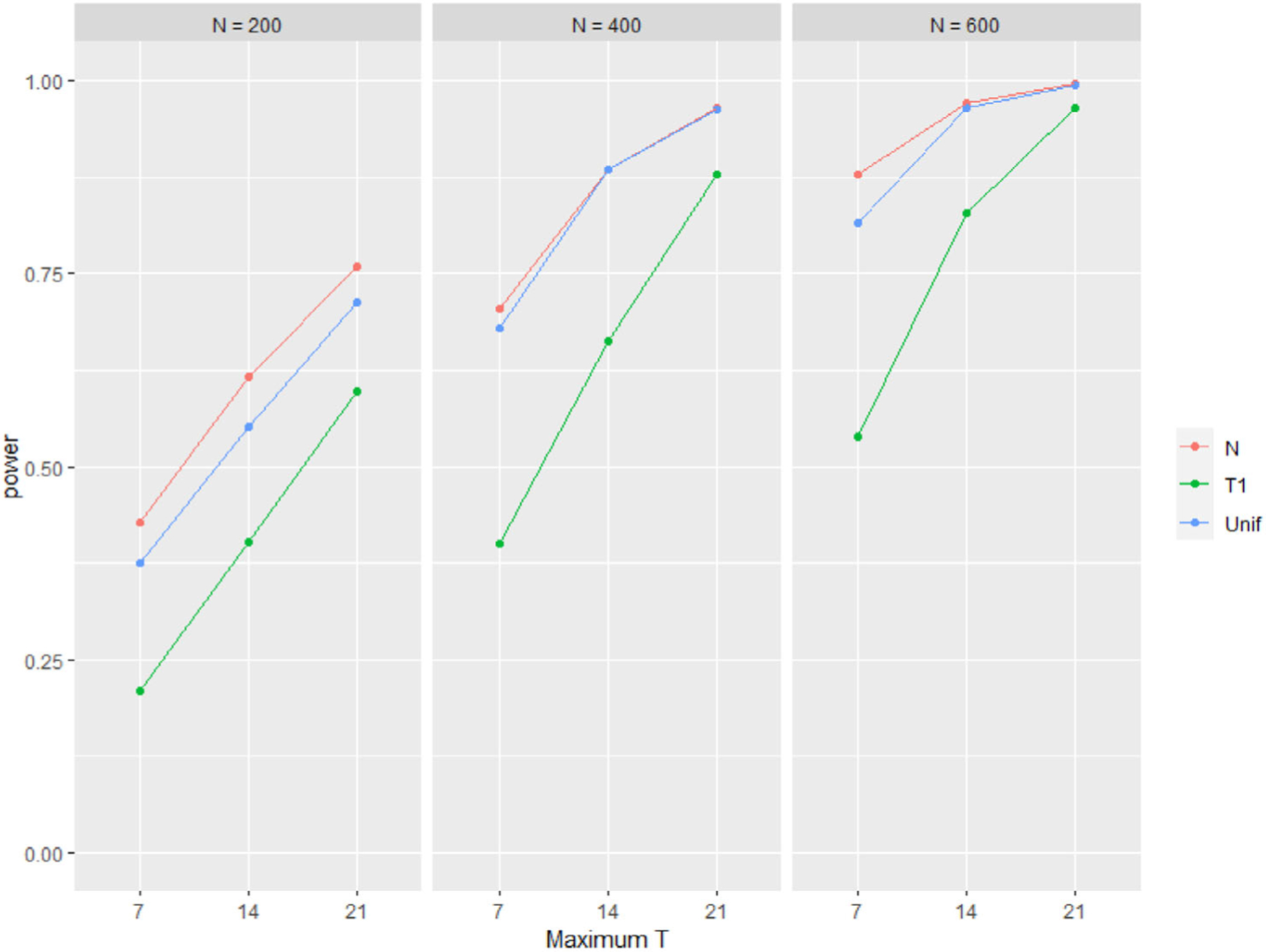
Power to detect the smallest beta coefficient (0.0309) in the Markov chain when the random effect is generated from a standard normal distribution (red), uniform distribution centered at 0 with variance 1 (blue), or Cauchy distribution (green) as a function of the number of subjects and maximum number of transitions for the th subject
4 |. APPLICATION TO COGNITIVE DATA
We analyze the cognitive data discussed by Abner et al. (2014) and Wang et al. (2021) to illustrate the proposed methodology. The data include 649 participates and the measurements are taken annually in the BRAiNs (Biologically Resilient Adults in Neurological Studies) cohort at the Alzheimer’s Disease Center of University of Kentucky (Schmitt et al., 2012). The goal of this analysis is to identify which groups are at low or high risk for the event of interest (e.g., relative risk of dementia). We assume a seven-state model where at each annual cognitive assessment a subject is placed into one and only one of the following seven state: intact cognition, A-MCI (amnestic MCI; mild cognitive impairment because of the weak performance on an annual memory test), M-MCI (mixed MCI; weak performance on a nonmemory cognitive exam; otherwise cognitively intact); MCI (mild cognitive impairment that is diagnosed by a clinician and verified by a low cognitive exam score and an informant); dropout before death or dementia; death without a diagnosis of a clinical dementia; diagnosis of clinical Alzheimer’s disease. Among these seven states, the first four are transient and the last three are absorbing, see Figure 2 for diagram illustration. That is, and . Figure 2 shows the one-step transitions possible between adjacent subject visits in this BRAiNs cohort study. The double-headed arrows indicate back transitions are possible from more impaired to less impaired states.
FIGURE 2.
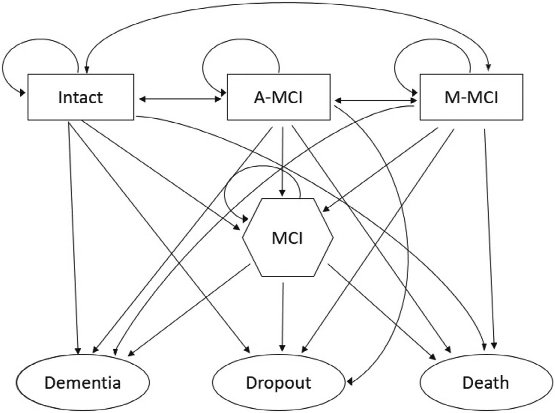
Flow diagram of one-step transitions between subjects visits. States are: intact (cognitively not impaired), A-MCI (test-based amnestic mild cognitive impairment), M-MCI (test-based nonamnestic mild cognitive impairment), MCI (clinical consensus mild cognitive impairment), dementia (clinical consensus dementia), dropout (participant drops out of study without incurring a dementia or dying), and death (participant dies without incurring a dementia)
The one-step transition probabilities among the states for the data is listed in Table 2. For each row, the number without parentheses (row 1) is the number of observed transitions and the number inside the parentheses (row 2) is the transition probability expressed as a percentage.
TABLE 2.
One-step transition matrix
| Current visit | ||||||||
|---|---|---|---|---|---|---|---|---|
| Last visit | Intact | A-MCI | M-MCI | MCI | Dementia | Dropout | Death | Total |
| Intact | 2634 (69.1) |
524 (13.8) |
464 (12.2) |
40 (1.1) |
15 (0.4) |
33 (0.9) |
101 (2.7) |
3811 (100) |
| A-MCI | 497 (57.6) |
172 (19.9) |
129 (15.0) |
23 (2.7) |
9 (1.0) |
13 (1.5) |
20 (2.3) |
863 (100) |
| M-MCI | 404 (30.7) |
97 (7.4) |
601 (45.7) |
66 (5.0) |
35 (2.7) |
30 (2.3) |
80 (6.2) |
1313 (100) |
| MCI | / / |
/ / |
/ / |
154 (61.4) |
50 (19.9) |
16 (6.4) |
31 (12.4) |
251 (100) |
Abbreviations: A-MCI, test-based amnestic mild cognitive impairment; M-MCI, test-based nonamnestic mild cognitive impairment; MCI, clinical consensus mild cognitive impairment.
To model this transition matrix, as Salazar et al. (2007) suggested, we assume the fixed effects are proportional for the transitions when the prior states are Intact cognition, A-MCI and MCI. For example, the fixed effect and are the same from our definition in Equation (4). To count for the information from the prior states, we included two indicator variables, see next paragraph for details. However, this assumption does not hold when the prior state is MCI because we have fewer transitions. Thus, the unknown parameter vector is .
We assume that the transition probabilities are dependent on baseline age (centered at age 74), gender, indication for low education (≤ 12 years) and the presence/absence of Apolipoprotein-E gene allele(s) (APOE4; a common risk factor for Alzheimer’s disease). Except these clinical covariates, we included two indicator variables printact (equals to 1 when the prior state is Intact and 0 otherwise) and pramnestic (equals to 1 when the prior state is A-MCI and 0 otherwise).
In this model we assume that for subject each transition probability relies on the fixed effects and one random effect . We further assume that for subject random effect follows a normal distribution with mean 0 and variance . We then use the step 1 in Section 2 to get the estimates for the fixed effects along with the standard errors. The resulting estimates of the fixed effects can be found in Tables 3 and 4. Along with the estimates for the fixed effects, we also estimated the standard deviation used for the random effect distribution . Since we assumed a scalar random effect with normal distribution, the PROC NLMIXED function in SAS system is used to optimize the approximated log likelihood function.
TABLE 3.
Parameter estimates with intact cognition as reference category when prior states are intact, A-MCI, M-MCI
| Risk factor | A-MCI | M-MCI | MCI | Dementia | Dropout | Death |
|---|---|---|---|---|---|---|
| Intercept | −1.225 * (0.182) |
−2.175 * (0.184) |
−4.717 * (0.391) |
−7.337 * (0.669) |
−3.613 * (0.309) |
−4.701 * (0.485) |
| Baseline age | 0.029* (0.007) |
0.073* (0.006) |
0.133* (0.014) |
0.164* (0.020) |
0.171* (0.012) |
0.056* (0.017) |
| Gender | −0.196 (0.103) |
0.121 (0.100) |
−0.185 (0.199) |
0.551 (0.317) |
−0.383 * (0.165) |
0.097 (0.257) |
| Low Education | 0.047 (0.164) |
0.597* (0.137) |
0.541* (0.265) |
−0.306 (0.478) |
0.188 (0.252) |
0.424 (0.337) |
| APOE4 | −0.081 (0.112) |
0.067 (0.105) |
0.603* (0.204) |
1.038* (0.283) |
−0.076 (0.192) |
0.171 (0.264) |
| Printact | 0.240* (0.109) |
0.060 (0.120) |
0.737* (0.272) |
0.835 (0.431) |
−0.341 (0.257) |
0.4272 (0.334) |
| Pramnestic | −0.257 (0.136) |
1.563* (0.100) |
1.723* (0.218) |
2.071* (0.322) |
0.977* (0.173) |
1.259* (0.267) |
Note: The values above the parentheses are the mle for the fixed effects and the values inside of the parentheses are the corresponding SEs.
Abbreviations: A-MCI, test-based amnestic mild cognitive impairment; M-MCI, test-based nonamnestic mild cognitive impairment; MCI, clinical consensus mild cognitive impairment.
TABLE 4.
Parameter estimates with MCI as reference category when prior states is MCI
| Risk Factor | Dementia | Dropout | Death |
|---|---|---|---|
| Intercept | −3.236 * (0.721) |
−3.263 * (0.833) |
−2.547 * (0.975) |
| Baseline age | 0.060* (0.029) |
0.110* (0.038) |
0.062 (0.049) |
| Gender | 0.708 (0.389) |
0.389 (0.459) |
−0.281 (0.573) |
| Low Education | −0.454 (0.487) |
−0.799 (0.644) |
−1.310 (1.020) |
| APOE4 | 0.823* (0.340) |
0.474 (0.0.483) |
0.300 (0.626) |
Note: The values above the parentheses are the mle for the fixed effects and the values inside of the parentheses are the corresponding SEs.
Given the estimates for the fixed effects, we are able to estimate the random effect through the method discussed in steps 2 and 3 of Section 2. All the computing work for steps 2 and 3 are conducted in . We summarize the results based on the random effects in the next paragraph.
We first notice that the probability of moving away from the reference state (intact cognitive) towards an impairment, death or drop out increases as the value for random effect increases. Based on this fact, we compare the top 5% to the bottom 5% and the middle 90% of the values. The thresholds for the division are 0.235 and −0.226. More specifically, a subject is within the top 5% if and is within the bottom 5% if and is within the middle 90% if stands between these two numbers. Table 5 shows the difference for the covariates and the number of transitions for the three groups. When comparing categories, we found that at baseline younger participants had fewer transitions than older participants (it further helps to show that the group with top random effect are quick to a terminating event). Table 6 shows the prior states distributions across the three groups and found that the Top 5% were more likely to start in the M-MCI. This results is consistent with the one-step transition matrix where the probability of a transition to dementia or death is larger when the prior state is M-MCI compared to intact cognition and A-MCI. Table 7 shows the distributions of the final states for the three comparison groups. The percentage of terminating events have large differences in these three groups (e.g., 90.9% for the bottom 5% group, 69.0% for the middle 90% group and 78.7% for the top 5% group). In addition, we found that the older subjects were more likely to dropout during follow-up.
TABLE 5.
Covariates differences based on the random effects
| Category | N | Low education (%) | Female (%) | APOE4(%) | Base age | Number of transitions |
|---|---|---|---|---|---|---|
| Bottom 5% | 33 | 6.1 | 60.6 | 21.1 | 85.4 ± 5.5 | 9.1 ± 4.7 |
| Middle 90% | 583 | 13.6 | 63.6 | 30.2 | 73.5 ± 7.0 | 9.9 ± 4.4 |
| Top 5% | 33 | 12.1 | 72.7 | 42.4 | 71.4 ± 5.8 | 5.5 ± 3.9 |
| p-Value | / | .46 | .53 | .17 | < .0001 | < .0001 |
TABLE 6.
Initial state based on the random effects
| Category/prior state | Intact cognitive | A-MCI | M-MCI |
|---|---|---|---|
| Bottom 5% | 69.7% | 12.1% | 18.2% |
| Middle 90% | 65.8% | 11.3% | 22.9% |
| Top 5% | 24.2% | 24.2% | 51.5% |
| p-value < .0001 |
Abbreviations: A-MCI, test-based amnestic mild cognitive impairment; M-MCI, test-based nonamnestic mild cognitive impairment.
TABLE 7.
Final state distributions based on the random effects
| Category/prior state | Intact cognitive | A-MCI | M-MCI | MCI | Dementia | Dropout | Death |
|---|---|---|---|---|---|---|---|
| Bottom 5% | 6.1% | 0.0% | 3.0% | 0.0% | 9.1% | 78.8% | 3.0% |
| Middle 90% | 23.5% | 1.2% | 4.8% | 5.5% | 16.8% | 38.5% | 13.7% |
| Top 5% | 0.0% | 0.0% | 21.2% | 0% | 24.2% | 21.2% | 33.3% |
| p-value <.0001 |
Abbreviations: A-MCI, test-based amnestic mild cognitive impairment; M-MCI, test-based nonamnestic mild cognitive impairment; MCI, clinical consensus mild cognitive impairment.
Besides the results here, we also checked other risk factors that are not included in the model. From the check, we found among females use of HRT (hormone replacement therapy reported at baseline) is more prevalent in the top category: 13/24 or 54.2% top, 116/371 or 31.3% middle and 3/20 or 15.5% bottom (-value = .0195 by Fisher’s Exact test). All other risk factors not in the fitted model had no relationship to the categories above; this includes indicators for smoking history, baseline diabetes, use of hypertensive medications, use of statin medications, history of head injury, and a body mass index above 25.
To determine if the normality assumption for the is reasonable, Studentized residuals defined as over the SD of were also examined. This set of 649 studentized residuals had mean value −0.096 with SD 0.569. The set passed a test for normality (e.g., Shapiro Wilk statistic is 0.997, -value = .25). Also, plots of these residuals indicate one possible outlier; see the plots in Figures 3 and 4.
FIGURE 3.
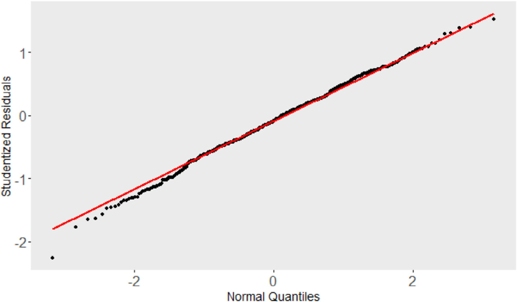
Normal quantile plot of the studentized residuals
FIGURE 4.
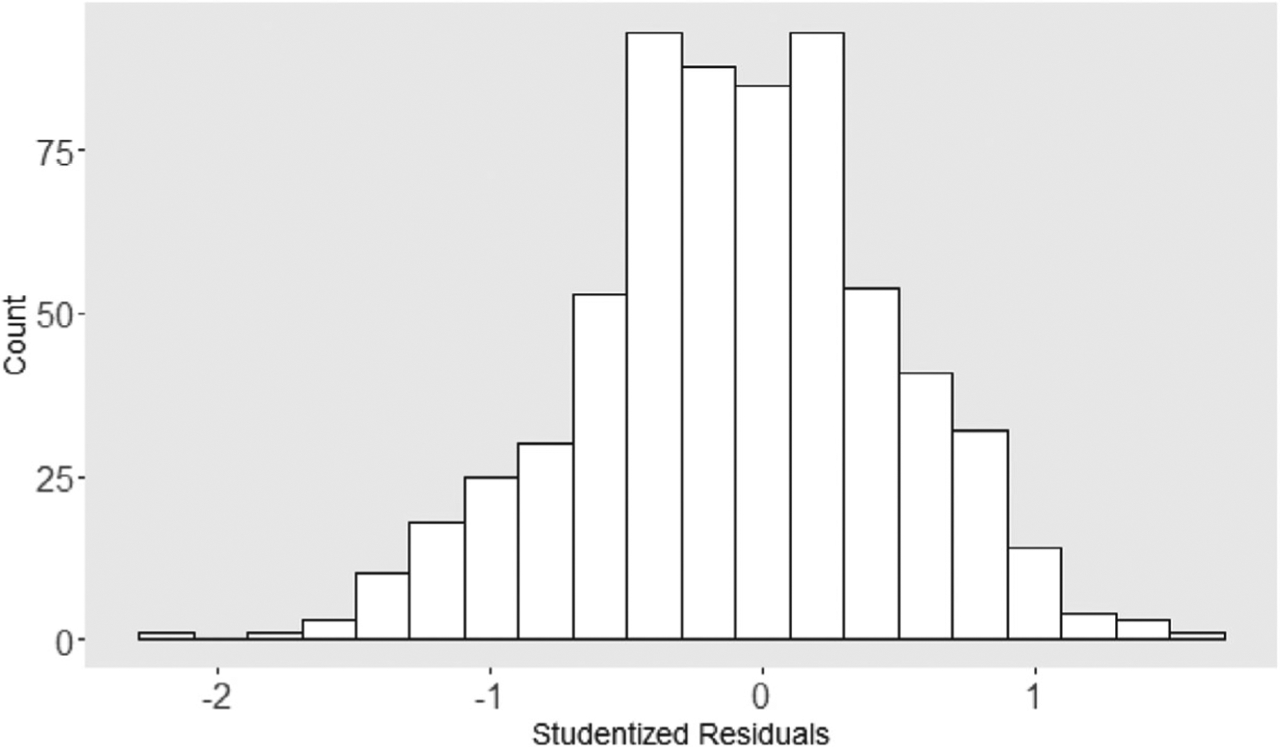
Distribution of the studentized residuals
The 95% confidence interval for the random effects are also plotted in Figure 5. From the plot, we identified the one possible outlier belongs to a subject with standardized residual −2.26 and the corresponding 95% confidence interval is (−4.22, −0.30). Upon further investigation, this subject is a male, age 68 at baseline, with 16 years of education, a non-APOE4 carrier, no diabetes, no head injury but a positive smoking history, BMI = 29.5, and taking statin and blood pressure medications (hence, cardiovascular risk). This subject had one baseline visit (declared nonamnestic MCI for age at that visit) and then (immediately) transitioned to dementia.
FIGURE 5.
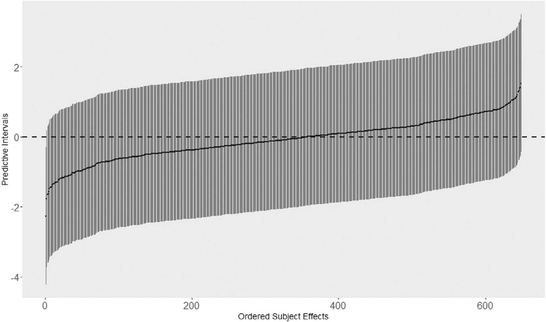
Predictive intervals (95% confidence intervals) based on ordering of the studentized residuals
5 |. DISCUSSION
In this paper we propose a h-likelihood method to estimate the fixed and random effects in a GLMM defined by a series of multinomial distributions that determine the one step transition probabilities in a finite Markov chain with transient states. The observations are a series of states in the chain visited by each experimental unit (persons at risk for a cognitive impairment in our example) which forms a cluster of correlated observations sharing a common random effect in the model. This is an example of a multistate transitional model. The estimation proceeds in steps with the first being the estimation of the fixed effects by maximizing the familiar marginal likelihood obtained after integrating out the random effects. The second step maximizes the joint likelihood to estimate the random effects by substituting the maximum likelihood estimators for the fixed effects into this joint likelihood. The third step also yields estimates of the SEs associated with each random effect allowing for the computation of studentized residuals. Using these residuals outliers are easily identified as are subsets of the experimental units that that are on a fast track or slow track for transitions into an absorbing state.
Model fitting is not necessarily straightforward at either step. When the random effect is a scalar and is normally distributed standard software may be used to do the integration needed to fit the marginal model to data. For example, PROC NLMIXED in the SAS system will fit the marginal model using an adaptive Gauss-Hermite quadrature with the option to use an importance sampling (Pinheiro & Bates, 1995). Other options include Monte-Carlo integration (Skrondal & Rabe-Hesketh, 2004) and a second-order Taylor series. Salazar et al. (2007) compared these methods in a simulation study in which the random effect was possibly nonnormally distributed. Another option is to use a probability integral transformation to normality when the random effect is nonnormally distributed (Nelson et al., 2006). As far as we know there is no software to fit the random effects to the h-likelihood once the fixed effects have been estimated.
The study of power or estimation in a GLMM usually depends on the choice of , the number of subjects, and , the number of observations for the th subject which is assumed to be of constant size. In a finite Markov chain with absorbing states multiple possible outcomes at each transition introduces additional complexities that need consideration in power/estimation studies especially if and is small. The number of transitions for a subject may be less than planned due to early absorption. Also, the occurrence of sparse or empty cells in the one step frequency matrix for the chain (Table 2) will create convergence problems when estimating the beta coefficients in Equation (6) or may lead to 0 for the estimate of the variance of the random effect. In the example presented in Section 4 the median value of is 9 (IQR: 7–21) and 91.4% of the individuals in the study have . As discussed in Lee et al. (2018) uniformly small cluster sizes can lead to biased estimates in the presence of binary responses which could be partially offset with the presence of additional covariates. It is more difficult to make equivalent summary statements in a finite Markov chain.
In this manuscript the model assumes one random effect, a random intercept. Multiple random effects are possible including the popular random intercept, random slope model. This would require integrating a two-dimensional integral in Step 1 which can still be facilitated using a multidimensional version of the Gauss quadrature algorithm. See, for example, Bartolucci et al. (2012) for a discussion of this case. When the dependent variable is assumed to be an indicator of an unobserved trait a latent Markov chain model can be assumed as well. The special case when the dependent variable is measured on an ordinal scale (e.g., a Likert scale which leads to a general logit model with an autoregressive process of order 1 over time) is discussed in the literature (Bartolucci, Montanari, & Pandolfi, 2015; Bartolucci, Bacci, & Pennoni, 2014) and has been generalized to the case where the respondent to a longitudinal survey consists of a set of indicator variables for the underlying latent response. In the latter case an additional step precedes Step 1 in which latent transition analysis is used to identify a small number of paths the cohort may follow over time (Bartolucci et al., 2015). This additional step is avoided in our application because the cognitive states and transitions among them are determined by a consensus conference that summarizes the result of a large neuropsychological battery given annually as well as supporting instruments measuring quality of life and depressive status, and reports by a close informant on the cognitive status of the participant during the previous year. An important point is that in all of this literature, the estimation of the random effects depends largely on the use of empirical Bayes which then raises additional assumptions related to choice of priors including prior distributions for the fixed effects in Step 1. For the random effects it also introduces additional notation related to posterior distributions, predictive densities, credible intervals, and caterpillar plots (Montanari, Doretti, & Bartolucci, 2018). The analytical procedure recommended in this manuscript avoids the additional Bayesian notation since all model parameters, fixed and random, are estimated by maximum likelihood.
The simulation study in Section 4 evaluated estimation and hypothesis testing for the fixed effects (Step 1 of the algorithm) under misspecification of the distribution of the random effects; that is, under a non normal distribution for the random effect (see, e.g., Litière, Alonso, & Molenberghs, 2007). It did not consider the effect of misspecification in Steps 2 and 3 because the sample residuals are noninformative on the normal distribution assumption for the random effects in hierarchical models (Alonso, Litière, & Laenen, 2010). These references relied on an empirical Bayes method to estimate the random effects and that method is well known to be subject to shrinkage toward zero. Paik, Lee, and Ha (2015) discuss using a frequentist approach to estimate the random effects when relying on maximum likelihood to produce the estimates. They showed that asymptotically these estimates are not necessarily normally distributed especially if the usual information matrix is used to estimate the standard errors of the random effects. To study random effects in GLMMs they suggest fixing the random effects across all simulations and treating these as fixed effects when evaluating estimation. This suggestion did not work well in the Markov chain model where shrinkage remained a problem.
A reviewer pointed out that the likelihood could be expanded to include the initial state which would involve using a multinomial model for determining entry into one of the transient states. This model would account for the covariates and would involve a subject specific random intercept that is shared with the random intercept in Equation (3). We followed this suggestion for the BRAiNS data example and found that it did not change the results much. Specifically, for the 31 beta coefficients that are listed as statistically significant in Tables 3 and 4 the percent error had a median value of 0.20% (IQR 5.4%) when each beta estimated without accounting for the initial state is compared to the same beta coefficients when the likelihood does account for the initial state. None of the nonsignificant betas in those tables changed to significant. This finding is consistent with that reported for the fixed effects in another dataset analyzed by Yu et al. (2010). In addition, for the 649 subjects in the BRAiNS dataset the difference between the random intercept estimated per subject which accounted for the initial state compared to that estimated by our method had a median value of 0.00024 (IQR 0.044). The entries in Tables 5–7 changed little and none of the conclusions from those tables changed. However, the inclusion of the initial state did identify one additional outlier; a 89-year-old male at baseline with 13 years of education and an APOE 4 carrier who had a severe head injury and cardiovascular risks (on a statin and blood pressure medications); that person had an intact cognition at baseline but transitioned to dementia within a year.
ACKNOWLEDGMENTS
This research was partially supported by grant UL11 TR001998 from the National Center for Advancing Translational Sciences and grants AG0386561, AG072946, and AG057191 from the National Institute on Aging.
Footnotes
CONFLICT OF INTEREST
The authors declare no potential conflicts of interest.
DATA AVAILABILITY STATEMENT
The data that support the findings of this study are available from the corresponding author upon reasonable request.
REFERENCES
- Abner EL, Nelson PT, Schmitt FA, Browning SR, Fardo DW, Wan L, … Kryscio RJ (2014). Self-reported head injury and risk of late-life impairment and ad pathology in an ad center cohort. Dementia and Geriatric Cognitive Disorders, 37(5–6), 294–306. [DOI] [PMC free article] [PubMed] [Google Scholar]
- Abramowitz M, Stegun IA, & Romer RH (1988). Handbook of mathematical functions with formulas, graphs, and mathematical tables. Maryland: American Association of Physics Teachers. [Google Scholar]
- Albert PS, & Follmann DA (2003). A random effects transition model for longitudinal binary data with informative missingness. Statistica Neerlandica, 57(1), 100–111. [Google Scholar]
- Alonso A, Litière S, & Laenen A (2010). A note on the indeterminacy of the random-effects distribution in hierarchical models. The American Statistician, 64(4), 318–324. [Google Scholar]
- Bartolucci F, Bacci S, & Pennoni F (2014). Longitudinal analysis of self-reported health status by mixture latent auto-regressive models. Journal of the Royal Statistical Society: Series C: Applied Statistics, 63(2), 267–288. [Google Scholar]
- Bartolucci F, Farcomeni A, & Pennoni F (2012). Latent Markov models for longitudinal data. Baco Raton, Florida: Chapman and Hall press. [Google Scholar]
- Bartolucci F, Montanari GE, & Pandolfi S (2015). Three-step estimation of latent markov models with covariates. Computational Statistics & Data Analysis, 83, 287–301. [Google Scholar]
- Bayarri M, DeGroot M, & Kadane J (1988). What is the likelihood function? Statistical decision theory and related topics IV (Vol. 1). New York, NY: Springer. [Google Scholar]
- Berger JO, & Wolpert RL (1988). The likelihood principle. Beachwood, Ohio: Institute of Mathematical Statistics. [Google Scholar]
- Bjørnstad JF (1996). On the generalization of the likelihood function and the likelihood principle. Journal of the American Statistical Association, 91(434), 791–806. [Google Scholar]
- Butler RW (1986). Predictive likelihood inference with applications. Journal of the Royal Statistical Society: Series B: Methodological, 48(1), 1–23. [Google Scholar]
- Chen H-HT, Yen M-F, Shiu M-N, Tung T-H, & Wu H-M (2004). Stochastic model for non-standard case-cohort design. Statistics in Medicine, 23(4), 633–647. [DOI] [PubMed] [Google Scholar]
- Gelfand AE, & Smith AF (1990). Sampling-based approaches to calculating marginal densities. Journal of the American Statistical Association, 85(410), 398–409. [Google Scholar]
- Hammersley JM, & Morton KW (1954). Poor man’s monte carlo. Journal of the Royal Statistical Society: Series B: Methodological, 16(1), 23–38. [Google Scholar]
- Lauritzen SL (1974). Sufficiency, prediction and extreme models. Scandinavian Journal of Statistics, 1(3), 128–134. [Google Scholar]
- Lee Y, & Nelder JA (1996). Hierarchical generalized linear models. Journal of the Royal Statistical Society: Series B: Methodological, 58(4), 619–656. [Google Scholar]
- Lee Y, & Nelder JA (2001). Hierarchical generalised linear models: A synthesis of generalised linear models, random-effect models and structured dispersions. Biometrika, 88(4), 987–1006. [Google Scholar]
- Lee Y, Nelder JA, & Pawitan Y (2018). Generalized linear models with random effects: Unified analysis via H-likelihood. Boca Raton, Florida: Chapman and Hall Press. [Google Scholar]
- Litière S, Alonso A, & Molenberghs G (2007). Type i and type ii error under random-effects misspecification in generalized linear mixed models. Biometrics, 63(4), 1038–1044. [DOI] [PubMed] [Google Scholar]
- Montanari GE, Doretti M, & Bartolucci F (2018). A multilevel latent markov model for the evaluation of nursing homes’ performance. Biometrical Journal, 60(5), 962–978. [DOI] [PubMed] [Google Scholar]
- Muenz LR, & Rubinstein LV (1985). Markov models for covariate dependence of binary sequences. Biometrics, 41(1), 91–101. [PubMed] [Google Scholar]
- Nelson KP, Lipsitz SR, Fitzmaurice GM, Ibrahim J, Parzen M, & Strawderman R (2006). Use of the probability integral transformation to fit nonlinear mixed-effects models with nonnormal random effects. Journal of Computational and Graphical Statistics, 15(1), 39–57. [Google Scholar]
- Paik MC, Lee Y, & Ha ID (2015). Frequentist inference on random effects based on summarizability. Statistica Sinica, 25(3), 1107–1132. [Google Scholar]
- Pinheiro JC, & Bates DM (1995). Approximations to the log-likelihood function in the nonlinear mixed-effects model. Journal of Computational and Graphical Statistics, 4(1), 12–35. [Google Scholar]
- Rosenbluth MN, & Rosenbluth AW (1955). Monte carlo calculation of the average extension of molecular chains. The Journal of Chemical Physics, 23(2), 356–359. [Google Scholar]
- Salazar JC, Schmitt FA, Yu L, Mendiondo MM, & Kryscio RJ (2007). Shared random effects analysis of multi-state markov models: Application to a longitudinal study of transitions to dementia. Statistics in Medicine, 26(3), 568–580. [DOI] [PubMed] [Google Scholar]
- Schmitt FA, Nelson PT, Abner E, Scheff S, Jicha GA, Smith C, … Kryscio RJ (2012). University of Kentucky sanders-brown healthy brain aging volunteers: Donor characteristics, procedures and neuropathology. Current Alzheimer Research, 9(6), 724–733. [DOI] [PMC free article] [PubMed] [Google Scholar]
- Skrondal A, & Rabe-Hesketh S (2004). Generalized latent variable modeling: Multilevel, longitudinal, and structural equation models. Baco Raton, Florida: Chapman and Hall/CRC. [Google Scholar]
- Song C, Kuo L, Derby CA, Lipton RB, & Hall CB (2011). Multi-stage transitional models with random effects and their application to the einstein aging study. Biometrical Journal, 53(6), 938–955. [DOI] [PMC free article] [PubMed] [Google Scholar]
- Tyas SL, Salazar JC, Snowdon DA, Desrosiers MF, Riley KP, Mendiondo MS, & Kryscio RJ (2007). Transitions to mild cognitive impairments, dementia, and death: Findings from the nun study. American Journal of Epidemiology, 165(11), 1231–1238. [DOI] [PMC free article] [PubMed] [Google Scholar]
- Vaida F, & Meng X (2004). Mixed linears models and the em algorithm in applied bayesian and causal inference from an incomplete data perspective. New York: John Wiley and Sons. [Google Scholar]
- Wang P, Abner EL, Fardo DW, Schmitt FA, Jicha GA, Van Eldik LJ, & Kryscio RJ (2021). Reduced rank multinomial logistic regression in Markov chains with application to cognitive data. Statistics in Medicine, 40(11), 2650–2664. [DOI] [PMC free article] [PubMed] [Google Scholar]
- Yu L, Griffith WS, Tyas SL, Snowdon DA, & Kryscio RJ (2010). A nonstationary markov transition model for computing the relative risk of dementia before death. Statistics in Medicine, 29(6), 639–648. [DOI] [PMC free article] [PubMed] [Google Scholar]
- Yun S, & Lee Y (2004). Comparison of hierarchical and marginal likelihood estimators for binary outcomes. Computational Statistics & Data Analysis, 45(3), 639–650. [Google Scholar]
Associated Data
This section collects any data citations, data availability statements, or supplementary materials included in this article.
Data Availability Statement
The data that support the findings of this study are available from the corresponding author upon reasonable request.