Exact Decoding of a Sequentially Markov Coalescent Model in Genetics

Abstract

In statistical genetics, the sequentially Markov coalescent (SMC) is an important family of models for approximating the distribution of genetic variation data under complex evolutionary models. Methods based on SMC are widely used in genetics and evolutionary biology, with significant applications to genotype phasing and imputation, recombination rate estimation, and inferring population history. SMC allows for likelihood-based inference using hidden Markov models (HMMs), where the latent variable represents a genealogy. Because genealogies are continuous, while HMMs are discrete, SMC requires discretizing the space of trees in a way that is awkward and creates bias. In this work, we propose a method that circumvents this requirement, enabling SMC-based inference to be performed in the natural setting of a continuous state space. We derive fast, exact procedures for frequentist and Bayesian inference using SMC. Compared to existing methods, ours requires minimal user intervention or parameter tuning, no numerical optimization or E-M, and is faster and more accurate.

1. Introduction

Probabilistic models of evolution have played a central role in genetics since the inception of the field a century ago. Beginning with foundational work by Ronald Fisher and Sewall Wright, and continuing with important contributions from P.A.P. Moran, Motoo Kimura, J.F.C. Kingman, and many others, a succession of increasingly sophisticated stochastic models were developed to describe patterns of ancestry and genetic variation found in a population. Statisticians harnessed these models to analyze genetic data, initially with the now quaint-seeming goal of understanding the evolution of a single gene. More recently, as next-generation sequencing has enabled the collection of genome-wide data from millions of people, interest has risen in methods for studying evolution using large numbers of whole genomes.

In this article, we study a popular subset of those methods which are likelihood-based; that is, these methods work by inverting a statistical model that maps evolutionary parameters to a probability distribution over genetic variation data. As we will see, exact inference in this setting is impossible owing to the need to integrate out a high-dimensional latent variable which encodes the genome-wide ancestry of every sampled individual. Consequently, a number of approximate methods have been proposed, which try to strike a balance between biological realism and computational tractability.

We focus on one such approximation known as the sequentially Markov coalescent (SMC). The sequential or “spatial” formulation of the coalescent was first derived by Wiuf and Hein (1999), and based on their ideas McVean and Cardin (2005) described an efficient Markovian algorithm for performing inference under a coalescent model with recombination. Although the term SMC is often used to refer to McVean and Cardin’s original algorithm, there are actually many methods in the literature that are simultaneously a) sequential, b) Markov, and c) approximations of the coalescent with recombination (McVean and Cardin, 2005, Marjoram and Wall, 2006, Carmi et al., 2014, Hobolth and Jensen, 2014). In this paper, we therefore use SMC more generally to refer to any method that meets these criteria. In particular, both the influential haplotype copying model of Li and Stephens (2003) and the popular program PSMC (Li and Durbin, 2011) for inferring population history are in the family of SMC methods under this definition (Paul and Song, 2010).

SMC models lead quite naturally to the use of hidden Markov models (HMMs) to analyze genetic sequence data. However, in order to bring the HMM machinery to bear on this problem, additional and somewhat awkward assumptions are needed. The latent variable in an HMM must have finite support, whereas the latent variable in SMC is a continuous tree. Therefore, the space of trees must be discretized, and, in some cases, restrictions must also be placed on the topology of each tree. In applications, the user must select a discretization scheme, a non-obvious choice which nonetheless has profound consequences for downstream inference (Parag and Pybus, 2019).

The main message of our paper is that this is not necessary: it is possible to solve a form of the sequentially Markov coalescent exactly, in its natural setting of continuous state space. We accomplish this by slightly modifying the canonical SMC model of McVean and Cardin (2005), in a way that does not greatly impact inference, but renders the problem theoretically and computationally much easier. In particular, this modification allows us to leverage recent innovations in changepoint detection, leading to algorithms which are computationally efficient and have reduced bias. Of course, some tradeoffs are necessary in order to achieve this: we must place some restrictions on the types of priors that can be used to model the instantaneous rate of coalescence, and, in contrast to existing approaches, the asymptotic running time of our algorithm is not known to us exactly. These restrictions, and their implications for inference, are explored in greater detail below.

The rest of the paper is organized as follows. In Section 2 we formally define our data and model, introduce notation, and survey related work. In Section 3 we derive our main results: exact and efficient Bayesian and frequentist algorithms for inferring genealogies from genetic variation data. In Section 4 we thoroughly benchmark our method, compare it to existing approaches, and provide an application to real data analysis. We provide concluding remarks in Section 5.

2. Background

In this section we introduce notation, formalize the problem we want to solve, and survey earlier work. We presume some familiarity with standard terminology and models in genetics; introductory texts include Hein et al. (2005) and Durrett (2008).

2.1. Motivation

Our method aims to infer a sequence of latent genealogies using genetic variation data. To motivate our interest in this, consider first a related problem with a more direct scientific application: given a matrix of DNA sequence data $\mathbf{Y}\in \{\mathrm{A},\mathrm{C},\mathrm{G},\mathrm{T}{\}}^{H\times N}$ from $H>1$ homologous chromosomes each $N$ base pairs long, and an evolutionary model $\phi$ hypothesized to have generated these data, find the likelihood $p(\mathbf{Y}\mid \phi )$. This generic formulation encompasses a wide variety of inference problems in genetics and evolutionary biology; if we could easily solve it, important new scientific insights would result.

Unfortunately, this is not possible using current methods. The difficulty lies in the fact that the relationship between the data $\mathbf{Y}$ and the scientifically interesting quantity $\phi$ is mediated through a complex, latent combinatorial structure known as the ancestral recombination graph (ARG; Griffiths and Marjoram, 1997), which encodes the genealogical relationships between every sample at every position in the genome. The ARG is sufficient for : evolution generates the ARG, and conditional on it, the data contain no further information about $\phi$. Thus, the likelihood problem requires the integration

$$p\left(Y\mid \phi \right)={\int }_{A\in 𝒜}p\left(Y\mid A\right)p\left(A\mid \phi \right),$$ (1)

where $A$ denotes an ARG, and $𝒜$ denotes the support set of ARGs for a sample of $H$ chromosomes. This is a very challenging integral; although a method for evaluating it is known (Griffiths and Marjoram, 1996), it only works for small data sets. That is because, for large $N$ and $H$, there are a huge number of ARGs that could have plausibly generated a given data set, such that the complexity of $𝒜$ explodes as $N$ and $H$ grow. Indeed, (1) cannot be computed for chromosome-scale data even for the simplest case $H=2$.

The sequentially Markov coalescent addresses this problem by decomposing the ARG into a sequence of marginal gene trees $X_1,\dots ,X_{N }$, one for each position in the chromosome, and supposing that this sequence is Markov. Then, we have

$$p\left(Y\mid \phi \right)\approx {\int }_{X_1,\dots ,X_N}\pi \left(X_1\mid \phi \right)p\left(Y_1\mid X_1\right)\prod _{n=2}^{N}p\left(Y_n\mid X_n\right)p\left(X_n\mid X_{n-1},\phi \right),$$ (2)

where $\pi (\cdot \mid \phi )$ is a stationary distribution for the Markov chain $X_1,\dots ,X_N$, the transition density $p\left(X_n\mid X_{n-1},\phi \right)$ governs the transition from one marginal tree to the next, and $\left[{\mathbf{Y}}_1|\cdots |{\mathbf{Y}}_N\right]=\mathbf{Y}$ are the data at each site.

Even under the Markov assumption, the integral (2) is challenging, since each $X_i$ represents a genealogy. To make the problem tractable, existing methods further assume that these genealogies have special structure. For example, in the widely used program PSMC (Li and Durbin, 2011), each “genealogy” has only two leaves, representing the ancestry of a pair of homologous chromosomes, so each $X_i\in {\mathbb{R}}_{\ge 0}$ can be taken to be a real number representing the height of the corresponding tree. The problem is then further simplified by discretizing time, such that the height of each tree falls into one of a pre-specified collection of discrete intervals. Similarly, the foundational Li-Stephens copying model (Li and Stephens, 2003) allows for more than two chromosomes to be analyzed, but assumes that the tree height is fixed to a single, pre-specified value and has a distinctive, “forest-of-trunks” structure (Paul and Song, 2010). In both cases, once the state space of the $X_i$ has been made finite, inference methods for hidden Markov models can be employed. Typically these are used to infer $\phi$ via the EM or Baum-Welch algorithm, which requires computing the posterior distribution

$$p\left(X_1,\dots ,X_N\mid Y,\phi \right).$$ (3)

2.2. Applications of the sequentially Markov coalescent

A number of noteworthy methods in statistical genetics and evolutionary biology depend on this model. Among the most widely used are methods for performing phasing and imputation (Scheet and Stephens, 2006, Marchini et al., 2007, Howie et al., 2009). Imputation methods leverage the fact that closely related members of a population tend to share genetic material to fill in missing genotype calls, and are an essential pre-processing step for improving power in genomewide association studies (Huang et al., 2015, Rubinacci et al., 2021). Phasing seeks to resolve diploid genotype calls, which, for technological reasons, are cheapest and easiest to produce, into constituent haplotypes. Phased haploid data is a necessary precursor for most evolutionary studies, and is also used to improve imputation accuracy (Howie et al., 2012). Crucially, through their underlying use of the Li-Stephens haplotype copying model (Li and Stephens, 2003), most existing phasing and imputation methods rely on accurate posterior estimates of local ancestry, $p\left(X_i\mid \mathbf{Y},\phi \right)$ in the notation of (3). We discuss this connection in further in Section 4.4.2.

Haplotype copying models are also directly used to study evolution, for example to estimate rates of recombination and gene conversion (Li and Stephens, 2003, Gay et al., 2007, Chan et al., 2012), to detect signatures of recent positive selection (Voight et al., 2006, Palamara et al., 2018), or to infer local ancestry (Price et al., 2009, Lawson et al., 2012). These methods aim to fit a particular evolutionary model $\phi$ to data using, essentially, equations (2) and (3), and frequentist or Bayesian model fitting procedures. For example, in their original paper Li and Stephens defined $\phi$ to be a sequence of local recombination rates (which enter into the likelihood through the transition density $p\left(X_n\mid X_{n-1},\phi \right)$ in (2)) and estimated $\hat{\phi }$ using the EM algorithm. Similarly, Palamara et al. (2018) compared local posterior distributions $p\left(X_i\mid \mathbf{Y},\phi \right)$, where $i$ indexes a particular location in the genome, to a genomewide null distribution in order to detect signatures of local adaptation within the last $~{10}^4$ years.

A problem of particular interest is so-called demographic inference (Spence et al., 2018), where $\phi$ represents historical fluctuations in population size. In this case, we can identify $\phi$ with a function $N_e:[0,\mathrm{\infty })\to (0,\mathrm{\infty })$, such that $N_e\left(t\right)$ is the coalescent effective population size $t$ generations before the present (Durrett, 2008, §4.4). This function governs the marginal distribution of coalescence time at a particular locus in a sample of two chromosomes. Specifically, setting $\eta \left(t\right)=1/N_e\left(t\right)$, the density of this time is

$$\pi \left(t\right)=\eta \left(t\right)e^{-{\int }_0^t\eta \left(s\right)ds}.$$ (4)

Note that $\eta \left(t\right)=1$ recovers the well-known case of Kingman’s coalescent, $\pi \left(t\right)=e^{-t}$, which we treat as the default prior in what follows.

Apart from intrinsic interest in learning population history, it is important to get a sharp estimate of $N_e\left(t\right)$ as unmodeled variability in $N_e\left(t\right)$ confound attempts to study some of evolutionary phenomena mentioned above, such as natural selection, or mutation rate variation. Many demographic inference methods have been proposed, using various underlying models and sources of data. One class (Gutenkunst et al., 2009, Bhaskar et al., 2015, Jouganous et al., 2017, Kamm et al., 2017, 2020) infers demographic history using so-called site frequency spectrum data, which is a low-dimensional summary statistic that is computed from mutation data assuming free recombination between markers. A second class of models, which includes ours, are designed to analyze whole-genome sequence data, and extract additional demographic signal from patterns of linkage disequilibrium. These methods are usually based on some form of the sequentially Markov coalescent (Li and Durbin, 2011, Sheehan et al., 2013, Rasmussen et al., 2014, Terhorst et al., 2017, Schiffels and Durbin, 2014, Steinrücken et al., 2019). Another recent development is the emergence of algorithms for inferring complete ancestral recombination graphs using large amounts of sequence data (Speidel et al., 2019, Kelleher et al., 2019), from which the demographic history can be estimated. Finally, there has been significant parallel work in phylogenetics on so-called skyline models, which are Bayesian procedures designed to infer population history under the assumption of a nonrecombining genealogy (Pybus et al., 2000, Drummond et al., 2005, Minin et al., 2008, Gill et al., 2013).

2.3. Our contribution

As discussed in Section 1, discretizing $X_i$ is unnatural and results in bias. In this work, we derive efficient methods for computing the posterior distribution $p\left(X_1,\dots ,X_N\mid \mathbf{Y}\right)$, or its maximum a posteriori estimate

$$\underset{X_1,\dots ,X_N}{\text{arg\hspace{0.17em}max\hspace{0.17em}}}p\left(X_1,\dots ,X_N\mid Y\right)$$

when each $X_i$ is a tree with continuous branch lengths. (To simplify the formulas, we suppress dependence on the evolutionary model $\phi$ until turning to inference in Section 4.4.) That is, unlike existing methods, we do not assume that the set of possible $X_i$ is discrete or finite. For the important case of $H=2$ chromosomes, our method is “exact” in the sense that it is devoid of further approximations (beyond the standard ones which we outline in the next section). In this case, the gene tree $X_i$ is completely described by the coalescence time of the two chromosomes. For $H>2$ our method makes additional assumptions about the topology of each $X_i$, but still retains the desirable property of operating in continuous time.

2.4. Notation and model

We now fix necessary notation and define the model that is used to prove our results. For simplicity, we first focus on the case of analyzing just one pair of chromosomes ($H=2$ in the notation of the previous section). In Section 3.4 we describe how to extend our results to larger sample sizes.

Assume that we have sampled a pair of homologous chromosomes each consisting of $N$ non-recombining loci. Meiotic recombination occurs between loci with rate $\rho$ per unit time, and does not occur within each locus. The number of generations backwards in time until the two chromosomes meet at a common ancestor (TMRCA) at locus $i$ is denoted $X_i\in {\mathbb{R}}_{>0}$. The number of positions where the two chromosomes differ at locus $i$ is denoted by $Y_i$. Under a standard assumption known as the infinite sites model (Durrett, 2008, §1.4), $Y_i$ has the conditional distribution

$$Y_i\mid X_i~\text{Poisson}\left(\theta X_i\right),$$

where $\theta$ is the mutation rate. We assume that both $\theta$ and $\rho$ are small. In particular, some of our proofs rely on the fact that $\rho \ll 1$. These are fairly mild assumptions which hold in many settings of interest. For example, in humans, the population-scaled rates of mutation and recombination per nucleotide are $O\left({10}^{-4}\right)$. Conversely, if recombinations are frequent, then there is little advantage in employing the methods we describe here, which depend on the presence of linkage disequilibrium between nearby loci.

The sequentially Markov coalescent is a generative model for the sequence $X_1,\dots ,X_{N }$, which we abbreviate as $X_{1:N}$ henceforth (and similarly for $Y_{1:N}$). SMC characterizes how shared ancestry changes when moving from one locus to the next. Assuming there is at most one recombination between adjacent loci, and we can specify an SMC model by the conditional density

$$f_{X_{n+1}\mid X_n}\left(t\mid s\right)≔p\left(X_{n+1}\in \left(t,t+dt\right)\mid X_n=s\right)=\delta \left(t-s\right)e^{-\rho s}+\left(1-e^{-\rho s}\right)q\left(t\mid s\right),$$ (5)

where $\delta (\cdot )$ is the Dirac delta function, and $q(t\mid s)$ is the conditional density of $t$ given that a recombination occurred and that the existing TMRCA equals $s$. Various proposals for $q(t\mid s)$ exist in the literature, each with slightly different properties (McVean and Cardin, 2005, Marjoram and Wall, 2006, Paul et al., 2011, Li and Durbin, 2011, Carmi et al., 2014). Importantly, they share the common feature that (5) is (approximately, in the case of Li and Durbin, 2011) reversible with respect to the coalescent. That is,

$$\pi \left(s\right)f_{X_{n+1}\mid X_n}\left(t\mid s\right)=\pi \left(t\right)f_{X_{n+1}\mid X_n}\left(s\mid t\right),$$ (6)

where $\pi$ is the stationary measure in equation (4). This can be verified in each of the above models by checking the detailed balance condition (Hobolth and Jensen, 2014).

2.5. Connection to changepoint detection

Our work is motivated by the observation that (5) is essentially a changepoint model. Indeed, SMC can be viewed as a prior over the space of piecewise constant functions spanning the interval $\left[0,N\right)$; conditional on realizing one such function, say $\xi :[0,N)\to [0,\mathrm{\infty })$, each $X_i=\xi (i-1)$, and the data $Y_{1:N}$ are independent Poisson draws with mean $\mathbb{E}\left(Y_i\mid X_i\right)=\theta X_i$. In genetics, each contiguous segment where $X_i=X_{i+1}=\cdots =X_{i+k-1}=\tau$, say, is known as an identity by descent (IBD) tract, with time to most recent common ancestor (TMRCA) $T$; the flanking positions where $X_{i-1}\ne X_i$ and $X_{i+k}\ne X_{i+k-1}$ are called recombination breakpoints. In changepoint detection, these are called segments, segment heights (or just heights), and changepoints, respectively. In what follows, we use these terms interchangeably depending on what is most descriptive in a given context.

A common assumption in changepoint detection is that neighboring segment heights are independent, which is to say that $X_i\perp X_{i+1}$ for any $i$ such that $X_i\ne X_{i+1}$. As we will see, this enables fast and accurate algorithms for inferring the sequence $X_{1:N }$. SMC violates this assumption through the conditional density $q(\mathrm{ }t \mid \mathrm{ }s )$ : the correlation between $t$ and $s$ in (5) makes the problem non-standard from a changepoint perspective. Although there has been recent work on detecting changepoints in data with dependence between segments (e.g., Fearnhead and Liu, 2011, Chan et al., 2021, Shi et al., 2022), particularly in time series, to the best of our knowledge the running time of these methods scales at least quadratically in the length of the underlying sequence.

In our application, sequence length is extremely long (a typical genetic sequence contains millions of observations), so methods with linear running time are essential. Perhaps the simplest way to achieve this is to approximate prior evolutionary model by one which ignores correlations in segment height. Indeed, if $q (\mathrm{ }t \mid \mathrm{ }s )$ were replaced by some function $\underset{\_}{\pi }\left(t\right)$ which did not depend on $s$, then (5) would become a so-called product partition model (PPM; Barry and Hartigan, 1992). In a PPM, a sequence of observations $y_1,\dots ,y_n$ is randomly partitioned into disjoint blocks $\left(y_1,\dots ,y_{b_1}\right),\left(y_{b_1+1},\dots ,y_{b_2}\right),\dots ,\left(y_{b_{k-1}+1},\dots ,y_{b_k}\right)$, such that the observations in each block are independent of all others. In the identity-by-descent problem described above, each block corresponds to an IBD segment, and the random partition has break points wherever recombinations occurred. PPMs are well-understood, and linear-time approximate methods have been developed to analyze them in both Bayesian (Barry and Hartigan, 1993, Fearnhead, 2006) and frequentist (Jackson et al., 2005, Killick et al., 2012) settings.

2.6. A renewal approximation

In biological applications, the orientation of the data sequence $Y_{1:N}$ is arbitrary; we could equivalently work with the reversed sequence $Y_N,Y_{N-1},\dots ,Y_1$ instead.

Additionally, both theoretical and empirical evidence overwhelmingly support that Kingman’s coalescent is a robust and accurate description of ancestry at a particular gene. For these reasons, it is important that any SMC model maintain the detailed balance condition (6). Given this desideratum, the obvious choice for $\underset{\_}{\pi }$ becomes

$$\underset{\_}{\pi }\left(t\right)\propto t\pi \left(t\right),$$ (7)

leading to the modified transition density

$$f_{X_{n+1}\mid X_n}^R\left(t\mid s\right)=\delta \left(t-s\right)e^{-\rho s}+\left(1-e^{-\rho s}\right)\underset{\_}{\pi }\left(t\right).$$ (8)

Checking the detailed balance condition (6), we obtain

$$\pi \left(s\right)\left(1-e^{-\rho s}\right)t\pi \left(t\right)\stackrel{?}{=}\pi \left(t\right)\left(1-e^{-\rho t}\right)s\pi \left(s\right),s\ne t.$$ (9)

Though (9) is not true in general, equality holds when both sides are expanded to first-order in $\rho$, which suffices for the applications we consider here.

The renewal approximation preserves an important piece of prior information concerning the nature of identity-by-descent: an IBD tract with TMRCA $x$ experiences recombination at rate $\rho x$, so more recent tracts are longer, a familiar fact to geneticists. On the other hand, prior information on the correlation between neighboring segment heights is dropped. We hypothesized that, for inference, it is more important that the prior capture the former effect than the latter. This is similar to the observation in changepoint detection that identifying changepoint locations tends to be harder than identifying the corresponding segment heights. Conditional on a given segmentation, finding the most likely segment heights is usually trivial, with a solution that depends mostly on the data and very little on the prior. Thus, it seems most important to encode prior information about the nature of the segmentation itself.

2.7. Prior work

The Markov chain defined by (8) was previously studied by Carmi et al. (2014), who coined the term renewal approximation. Carmi et al. derived theoretical results and performed simulations to study identity-by-descent patterns produced by SMC models. They found that the renewal approximation is comparable to other variants of SMC with some inaccuracy mainly in the tails of the IBD distribution. Importantly, these results pertain to the accuracy of these methods as priors; they do not necessarily imply that the renewal approximation is inferior for inference. Indeed, generally one hopes that “the data overwhelm the prior,” so that inferences do not depend strongly on the choice of prior model.

There have been a few papers specifically devoted to improving the efficiency of SMC. Harris et al. (2014) and Palamara et al. (2018) derived $O\left(MN\right)$ decoding algorithms for certain SMC models, where $M$ is the number of hidden states (time discretizations) used in the underlying hidden Markov model. Separately, Lunter (2019) recently showed that MAP estimation can be performed for the Li and Stephens model in $O\left(N\right)$ time irrespective of the size $H$ of the underlying copying panel, after a preprocessing step that costs $O\left(HN\right)$ time (Durbin, 2014).

3. Methods

In this section we derive exact representations for the sequence of marginal posterior distributions $p\left(X_n\mid Y_{1:N}\right),n=1, 2,\dots ,N$, and efficient algorithms for sampling paths from the posterior density $p\left(X_{1:N}\mid Y_{1:N}\right)$ and for computing the MAP path

$$X_{1:N}^{*}=\underset{X_{1:N}}{\text{arg\hspace{0.17em}max\hspace{0.17em}}}p\left(X_{1:N}\mid Y_{1:N}\right).$$

To save space, proofs are deferred to Appendices S1–S4 in the supplementary material. For the reader’s convenience, the various notations introduced in this section are listed in Table S1.

3.1. Exact marginal posterior

In what follows, we write $f\left(x\right)\in {ℳ}_{\mathrm{\Gamma }}\left(K\right)$ to signify a the probability density $f$ is a mixture of $K$ gamma distributions, with the mixing weights, scale and shape parameters left unspecified. By abuse of notation, we also write $X~{ℳ}_{\mathrm{\Gamma }}\left(K\right)$ to signify that the random variable $X$ is distributed according to such a mixture.

Let $\alpha \left(X_n\right)=p\left(X_n\mid Y_{1:n}\right)$ denote the (rescaled) forward function from the standard forward-backward algorithm for inferring hidden Markov models (Bishop, 2006, § 13.2.4). Our first result shows that, under the renewal approximation, $\alpha \left(X_n\right)$ is a mixture of gamma distributions.

Proposition 1. Suppose that $\pi \left(x\right)\in {ℳ}_{\mathrm{\Gamma }}\left(K\right)$. Then $\alpha \left(X_n\right)=p\left(X_n\mid Y_{1:n}\right)\in {ℳ}_{\mathrm{\Gamma }}\left(nK\right)$.

Using this result, we can derive a representation for the marginal posterior distribution.

Proposition 2. If $\pi \left(x\right)\in M_{\mathrm{\Gamma }}\left(K\right)$ then there exists $f\left(X_n\right)\in {ℳ}_{\mathrm{\Gamma }}\left(Kn\right)$ and $g\left(X_n\right)\in {ℳ}_{\mathrm{\Gamma }}\left(K\right(N-n\left)\right)$ such that

$$p\left(X_n\mid Y_{1:N}\right)=\frac{f\left(X_n\right)g\left(X_n\right)}{\pi \left(X_n\right)}.$$ (10)

We can also derive exact expressions for the mixing proportions, shape, and scale parameters for $p\left(X_n\mid Y_{1:n}\right)$, and by extension, the exact algebraic expression for $p\left(X_n\mid Y_{1:N}\right)$. This requires substantial additional notation and is deferred to Appendix S5.

3.2. Efficient posterior sampling

The exact posterior formula derived in Proposition 2 is useful for visualization, or numerically evaluating functionals (e.g., the posterior mean) of the posterior distribution. However, it is less suited to sampling since the denominator does not divide the numerator except when $K=1$; and even then, sampling requires expanding the numerator in (3) into (as many as) $O\left(K^2{N}^2\right)$ mixture components.

Instead, we provide an algorithm for efficiently sampling entire paths from $p\left(X_{1:N}\mid Y_{1:N}\right)$. This idea is due to Fearnhead (2006) (see also Barry and Hartigan (1992)), with necessary modifications to accommodate our model’s dependence between segment length and height.

Let $R_v$ denote the event that a new IBD segment begins at position $v$, let ${\overline{R}}_{u:v}≔{\left(\underset{i=u+1}{\overset{v-1}{\cup }}{R}_i\right)}^C$ denote the event that there is not a recombination event between positions $u$ and $v$ (exclusive), and set ${\overline{Y}}_{u:v}:=\sum _{i=u}^v{Y}_i$ The joint likelihood of the data $Y_{u:v}$ and the event that an IBD segment starts at position $u$ and extends $\mathrm{\Delta }=v-u+1$ positions before terminating at position $v$ is

$$p\left(Y_{u:v},{\overline{R}}_{u:v},R_v\right)={\int }_x{x}^{1_{\{u>1\}}}\pi (x)\rho x{e}^{-\rho \Delta x}\prod _{i=u}^v{e}^{-\theta x}{(\theta x)}^{Y_i}/Y_i!=:P(u,v).$$ (11)

A special case for $u=1$ is necessary because the initial segment height is sampled from the stationary distribution $\pi$, while successive segments heights are distributed according to $\underset{\_}{\pi }$; cf. equations 2 and 8.

For the last segment, we know only that it extended past position $N$, so we make the special definition

$$P_{-1}\left(u,N\right)=p\left(Y_{u:N},{\overline{R}}_{u:N}\right)={\int }_x{x}^{1_{\left\{u>1\right\}}}\pi \left(x\right)e^{-\rho \Delta x}\prod _{i=u}^N{e}^{-\theta x}{(\theta x)}^{Y_i}/Y_i!.$$ (12)

Our algorithm can be used whenever (11) can be efficiently evaluated, in particular when $\pi \left(t\right)$ is a gamma mixture.

Defining $Q\left(u\right)=p\left(Y_{u:N}\mid R_u\right)$ and integrating over the location $v$ where the segment originating at position $u$ terminates, we have (Fearnhead, 2006, Theorem 1)

$$Q\left(u\right)=\sum _{v=u}^{N-1}P\left(u,v\right)Q\left(v+1\right)+P_{-1}\left(u,N\right)$$ (13)

which can be solved by dynamic programming starting from $v=N-1$ in $O\left(N^2\right)$ time. When $v-u$ is large, $P(u,\mathrm{ }\mathrm{ }v)$ tends to be extremely small, so the summation in (13) can be truncated without loss of accuracy to obtain an algorithm which is effectively linear in $N$. Except when noted otherwise, we followed Fearnhead’s original suggestion, and truncated the summation as soon as $P(u,v)Q (v+1)$ was less than ${10}^{-4}$.

To sample the next recombination breakpoint ${\tau }^{\mathrm{\text{'}}}$ from the posterior given that the previous breakpoint occurred at location $\tau$, note that

$$\begin{gathered} p\left({\tau }^{\prime }\mid \tau ,Y_{1:N}\right)=\frac{p\left(Y_{1:N},R_{\tau },R_{{\tau }^{\prime }},{\overline{R}}_{\tau ,{\tau }^{\prime }}\right)}{p\left(Y_{1:N},R_{\tau }\right)} \\ =\frac{p\left(Y_{1:\tau -1},R_{\tau }\right)p\left(Y_{\tau :{\tau }^{\text{'}}-1},R_{{\tau }^{\text{'}}},{\overline{R}}_{\tau :{\tau }^{\text{'}}}\mid R_{\tau }\right)Q\left({\tau }^{\prime }\right)}{p\left(Y_{1:\tau -1},R_{\tau }\right)Q\left(\tau \right)} \\ =P\left(\tau ,{\tau }^{\prime }-1\right)Q\left({\tau }^{\prime }\right)/Q\left(\tau \right) \end{gathered}$$

for ${\tau }^{\mathrm{\text{'}}}=\tau +1,\dots ,N-1\mathrm{ }$, with the remaining probability mass placed on the event that there are no more changepoints. If sampling the first changepoint we set $T=1.$

Having sampled a segmentation $0<{\tau }_1,\dots ,{\tau }_K<N$ from the posterior, we then sample heights conditional on this segmentation. Given that observations $u,u+1,\dots ,v-1,v$ are all on the same segment and are flanked by recombinations, the joint probability of the data $Y_{u:v}$, the segment length $\mathrm{\Delta }$, and the segment height $x$, is the integrand in (11). Hence, the posterior distribution of the segment height $x$ conditional on the underlying segmentation is

$$p\left(x\mid {\overline{Y}}_{u:v},R_{u:v},R_v\right)\propto x^{1_{\{u>1\}}}\pi \left(x\right)\rho x{e}^{-\rho \text{Δ}x}{e}^{-\theta x}x\sum _{i=u}^v{Y}_i.$$ (14)

If $\pi \left(x\right)$ is a gamma (mixture), then (14) is also a gamma mixture, and hence easy to sample.

3.3. Exact frequentist inference

To complement the Bayesian results in the preceding section, we also derive an efficient frequentist method for inferring the maximum a posteriori (MAP) hidden state path,

$$X_{1:N}^{\text{*}}≔\underset{X_{1:N}}{\text{arg\hspace{0.17em}max\hspace{0.17em}}}p\left(X_{1:N},Y_{1:N}\right).$$ (15)

When $X_1,\dots ,X_N\in 𝒳$ have discrete support, $\mid 𝒳\mid =M$, the MAP path can be found in $O \left(N{M }^{2\mathrm{ }}\right)$ time using the Viterbi algorithm (Bishop, 2006), and in some cases in $O\left(NM\right)$ time by exploiting the special structure of the SMC (Harris et al., 2014, Palamara et al., 2018). Our goal is to efficiently solve the optimization problem (15) when $𝒳=ℝ>0$.

To accomplish this, we start by defining the recursive sequence of functions

$$V_1\left(t\right)=\text{log\hspace{0.17em}}\pi \left(t\right)+e_1\left(t\right)$$

$$V_n\left(t\right)=\underset{s}{\text{max\hspace{0.17em}}}{V}_{n-1}\left(s\right)+\varphi \left(t\mid s\right)+e_n\left(t\right),n\ge 2$$

$$V_n^{\text{*}}=\underset{t}{\text{max\hspace{0.17em}}}{V}_n\left(t\right)$$

where $e_i\left(t\right)=\text{log\hspace{0.17em}}p\left(Y_i\mid X_i=t\right)$, and

$$\begin{gathered} \varphi \left(t\mid s\right)=\text{log\hspace{0.17em}\hspace{0.17em}}p\left(X_{i+1}=t\mid X_i=s\right) \\ =\{\begin{array}{ll}-\rho t,\hfill & t=s\hfill \\ \text{log\hspace{0.17em}}\left(1-e^{-\rho s}\right)+\text{log\hspace{0.17em}\hspace{0.17em}}\underset{\_}{\pi }\left(t\right),\hfill & \text{ otherwise }\hfill \end{array} \\ \approx \{\begin{array}{ll}-\rho t,\hfill & t=s\hfill \\ \text{log\hspace{0.17em}}\left(\rho s\right)+\text{log\hspace{0.17em}}\underset{\_}{\pi }\left(t\right),\hfill & \text{ otherwise, }\hfill \end{array}\left(\rho \ll 1\right) \end{gathered}$$

This is the usual Viterbi dynamic program, but defined over a continuous instead of discrete domain. By standard arguments (Bishop, 2006, §13.2.5), we have

$$X_N^{\text{*}}=V_N^{\text{*}}=\underset{X_N}{\text{arg\hspace{0.17em}max}}\left[\underset{x_{1:N-1}}{\text{max}}p\left(X_{1:N},Y_{1:N}\right)\right],$$

and the full path $X_{1:N}^{\mathrm{*}}$ can be recovered by backtracing.

Thus, if we could calculate $V_n\left(t\right)$ then the optimization problem (15) would be solved. In general, it is not obvious how to accomplish this, since $V_n\left(t\right)$ is a function, i.e. an infinite-dimensional object which cannot be represented by a computer program. However, our next theorem shows that, in fact, each $V_n\left(t\right)$ has a finite-dimensional representation.

Definition 1. Let ${𝒱}_K$ be the space of all functions $f:[0,\mathrm{\infty })\to \mathbb{R}$ which can be piecewise defined by $K$ functions of the form $t\mapsto at+b\text{\hspace{0.17em}log\hspace{0.17em}}t+c$. That is, $f\in {𝒱}_K$ if and only if there exists there exists an integer $K$, a vector $\tau \in {\mathbb{R}}^{K+1}$ satisfying

$$0={\tau }_1<{\tau }_2<\cdots <{\tau }_{K+1}=\infty ,$$

and vectors $\mathbf{a},\mathbf{b},\mathbf{c}\in {\mathbb{R}}^K$ such that

$$f=a_{k}t+b_k\text{log\hspace{0.17em}}t+c_k,t\in \left[{\tau }_{k-1},{\tau }_k\right).$$

Proposition 3. Suppose that $N_e\left(t\right)\in {𝒱}_K$ is piecewise constant. Then for each $n=1,\dots ,N$, there exists $K_n<\mathrm{\infty }$ such that $V_n\left(t\right)\in {𝒱}_{K_n}$.

The proof of the theorem (Appendix S3) shows that in order to efficiently compute $V_n\mathrm{ }\left(t\right)$ we need to be able to take the pointwise maximum between any two functions in ${𝒱}_K$. We provide an $O\left(K\right)$ procedure for doing this in Appendix S6.

Our next result establishes the functional form of $V_n\left(t\right)$. Each piece of $V_n\left(t\right)$ comprises an interval $I\subset \mathbb{R}$ where, conditional on the TMRCA at position $n$ being $t\in I$, the most probable recombination event occurred a certain number of positions ago. In the statement and proof of the theorem, we use double brackets, $\left[\right[·\left]\right]$, to refer to individual entries of subscripted vectors.

Proposition 4. For each $V_n\left(t\right)$ , with breakpoints ${\tau }_n\in \mathbb{R} k_n+1$, there exists vectors $i_n\in {\mathbb{Z}}^{K_n}\ge 0$ and $C_n\in {ℝ}^{K_n}$ such that, for $t\in \left[{\tau }_n[[k]],{\tau }_n[[k+1]]\right)$,

$$V_n\left(t\right)=C_n\left[\left[k\right]\right]+\text{log\hspace{0.17em}}\underset{\_}{\pi }\left(t\right)+{\overline{Y}}_{i_n[\left[k\right]]:n}\text{\hspace{0.17em}log}\left(\theta t\right)-t\left(\theta +\rho \right)\left(n-i_n\left[\left[k\right]\right]\right)-\theta t.$$

Hence, up to the constant ${\mathbf{C}}_n\left[\right[k\left]\right],V_n\left(t\right)$ equals the log-likelihood of ${\overline{Y}}_{{\text{i}}_n\left[\left[k\right]\right]:n}$ given that the most recent recombination event occurred at position $\left.{\text{i}}_n\left[\right[k]\right]$ and $X_{\left.{\text{i}}_n\left[\right[k]\right]}=\cdots =X_n=t$.

Complete pseudocode for our algorithm, based on Propositions 3 and 4, is given in the supplement (Algorithm S1).

In Section 4.2, it will be seen that the posterior distribution is sometimes not centered over the MAP path: the latter tends to oversmooth, missing many changepoints, whereas the posterior mode/mean is generally close to the truth (Figure S5). This is a known feature of the Viterbi decoding of a hidden Markov model, and is not specific to our problem setting (Yau and Holmes, 2013, Lember and Koloydenko, 2014). In Appendix S7 we derive a generalization of Proposition 3 which allows us to efficiently compute other paths which are suboptimal with respect to (15), but have better pointwise accuracy, thus enabling a range of possible decodings.

3.4. Extension to larger sample sizes

The preceding sections focused on inferring the sequence of TMRCAs in a pair of sampled chromosomes. In modern applications where hundreds or thousands of samples have been collected, methods that can analyze larger sample sizes are desirable.

We can generalize the problem of decoding the pairwise TMRCA amongst two chromosomes by treating one of the chromosomes as a fixed genealogy, and considering where the other chromosome joins onto this genealogy at each position. Then, more generally, given a “panel” of $H\ge 1$ chromosomes, we can ask where at each position an additional “focal” chromosome joins onto the panel genealogy.

Extending sequentially Markov coalescent methods to larger sample sizes is not trivial for the simple reason that there is more than one possible tree topology to consider when $n>2$. Instead of inferring a sequence of numbers $X_{1:N}$ (representing the height of a tree with two leaves), as in the preceding sections, one must consider as hidden states the space of edge-weighted binary trees on $n$ leaves. To circumvent this difficulty, we employ a so-called trunk approximation (Paul and Song, 2010), which supposes that the underlying ancestral recombination graph is a disconnected forest of $H$ trunks extending infinitely far back into the past. The state space of this model is $\left\{1,\dots ,H\right\}\times ℝ>0$, where the first, discrete coordinate describes the panel haplotype onto which a focal haplotype is currently coalesced, and the second, continuous coordinate gives them time at which that coalescence occurrred. Although the trunk assumption is strong, it has proved useful in a variety of settings (Sheehan et al., 2013, Spence et al., 2018, Steinrücken et al., 2019).

Modifying our methods to utilize the trunk approximation is straightforward and amounts to, essentially, replacing the coalescence measure $p(X\in [t,t+dt\left)\right)=\pi \left(t\right)dt$ with the product measure $p\left(\right(X,h)\in ([t,t+dt),\left\{i\right\}\left)\right)=\pi \left(Ht\right)dt$ in all of our formulas. (Note that this measure is properly normalized.) In other words, coalescence occurs with each haplotype at rate 1, and conditional on coalescence, it occurs uniformly onto each haplotype.

4. Results

In this section we compare our method to existing ones, benchmark its speed and accuracy, and conclude with some applications.

4.1. Local ancestry inference is comparable to existing methods

As described in the introduction, our initial hypothesis was that posterior inferences for the haplotype decoding problem are relatively insensitive to the choice of prior model on the way that the sequentially Markov coalescent transitions from one position to the next. Here we confirm this hypothesis. To study the relationship between the posterior and prior, we compared the the renewal model developed above to the conditional Simonsen-Churchill (CSC) model of Hobolth and Jensen (2014). The CSC is the most accurate sequentially Markovian model known in the literature, and other models such as SMC (McVean and Cardin, 2005) and SMC’ (Marjoram and Wall, 2006) are further approximations of it. Hence, CSC and the renewal model can be viewed as the least and most approximative SMC methods, respectively.

To compare models, we used the procedure described in Hobolth and Jensen (2014, §4.4) to compute the transition probability matrix $T$, where

$$T_{ij}=p\left(X_{\ell +1}\in \left[t_j,t_{j+1}\right)\mid X_{\ell }\in \left[t_i,t_{i+1}\right)\right)$$

is the probability that the TMRCA at site $\ell +1$ is in the interval $\left[t_j,t_{j+1}\right)$ given that the TMRCA of an adjacent site is in $\left[t_i,t_{i+1}\right)$. We then used this transition matrix to perform posterior decoding in a discrete-state coalescent HMM as previously described (Li and Durbin, 2011). We compared the CSC and renewal prior under both constant population size and varying population size, as well as when the recombination rate is equal to the mutation rate and when it is lower. Taking all the combinations of the different population size histories and the recombination rate gives us a total of 4 scenarios. Scenarios 1 and 3 have constant population size, and scenarios 2 and 4 have the variable population size. Scenarios 1 and 2 have recombination rate $r={10}^{-9}$, and scenarios 3 and 4 have recombination rate $r=1.4\times {10}^{-8}$ per base-pair per generation. We bucketed consecutive base pairs into groups of size $w=100$ and assume that the recombinations occur between these groups. Additional details of our simulation can be found in Appendix S8.1.

Supplemental Figures S1 and S2 show the Viterbi path and the posterior heatmap for one run of each scenario of the simulation. From Figure S1, there is little difference in the Viterbi plot between the CSC and renewal priors. Both priors produce a Viterbi path very similar to the true sequence of TMRCAs. When the recombination rate increases, the Viterbi paths produced by the two priors fail to capture all the recombination events, but are still very similar in their outputs. We performed a similar analysis for the posterior decoding (Figure S2). Again, it is hard to discern any meaningful difference in all scenarios between the two priors. This is especially the case in scenarios 1 and 2 where the recombination rate is lower.

Confirming these qualitative observations, Table 1 shows the average absolute error for the two priors over the 25 simulations. In terms of absolute error, the renewal prior does about as well as the more correct CSC prior. In fact, the renewal prior outperforms CSC under scenarios 3 and 4, the scenarios with higher recombination rate. A potential explanation for this surprising result, suggested by visually inspecting the posterior decoding obtained from the two methods (e.g., Figure S2, bottom panel), is that the signal-to-noise level in the high recombination regime is low enough that ignoring correlations between (noisily) inferred adjacent segments can actually improve estimation. Provisionally, we hypothesize that the renewal approximation acts as a sort of shrinkage prior in the high-noise regime, trading some bias for lower average risk. However, we observed this effect in only a small number of high-recombination settings, and it is not as pronounced when considering relative error (Table S2).

Table 1.

Mean absolute error $\left(E{rr}_A\right)$ over 25 runs under each scenario. CSC results were obtained from the conditional Simonsen-Churchill model. Renewal results are from our method. Both methods were discretized. Standard error in parentheses.

Scenario	Constant Ne	Variable Ne	Constant Ne	Variable Ne
	Low ρ (1)	Low ρ (2)	High ρ (3)	High ρ (4)
CSC	5686.79 (198.96)	5201.35 (228.23)	12207.96 (316.49)	11949.15 (146.20)
Renewal	5683.52 (192.43)	5212.97 (226.64)	11660.02 (303.80)	11427.61 (147.19)

To better understand these results, we also stratified the error measure by quarter of the true TMRCA distribution (Tables 2 and S3). We expected to see a greater difference between the two priors for larger values of the true TMRCA since, under the CSC prior, the distribution of tree height of the current segment conditioned on the tree height of the previous segment, $q (t \mid \mathrm{ }s )$ is approximately uniform in $t$ for large $s$, i.e. $q \left(\mathrm{ }t ∣\mathrm{ }s \right)\approx 1\mathrm{ }/\mathrm{ }s$ when $s \gg \mathrm{ }t$, where under the renewal prior $\pi \left(t\right)={e }^{-t}$ has an exponential tail. Conversely, since $\underset{s\to 0}{\text{lim\hspace{0.17em}}}q(t\mid s)=e^{-t}$, the methods should be comparable for recent TMRCAs.

Table 2.

Mean absolute error $\left({\mathrm{E}\mathrm{r}\mathrm{r}}_A\right)$ over 25 runs under each scenario stratified by quartile. Other details are as in Table 1.

Scenario	Qtr.	Constant Ne	Variable Ne	Constant Ne	Variable Ne
		Low ρ (1)	Low ρ (2)	High ρ (3)	High ρ (4)
CSC	Q1	2676.74 (115.50)	2271.89 (126.87)	6932.49 (242.41)	6550.15 (118.46)
Renewal	Q1	2714.53 (117.88)	2330.01 (127.42)	5365.78 (184.23)	5168.37 (77.63)
CSC	Q2	5961.49 (111.73)	6263.63 (159.11)	13407.48 (60.54)	13255.75 (45.30)
Renewal	Q2	6061.91 (98.98)	6289.53 (147.09)	11575.83 (44.20)	11549.62 (29.92)
CSC	Q3	9679.44 (148.74)	9770.56 (259.23)	18853.84 (41.04)	18811.84 (58.56)
Renewal	Q3	9569.68 (156.41)	9673.67 (283.39)	19620.79 (71.97)	19470.72 (52.02)
CSC	Q4	15833.47 (265.34)	15968.86 (426.23)	33105.92 (170.73)	33412.66 (200.11)
Renewal	Q4	15439.84 (322.81)	15760.62 (527.12)	40368.10 (208.78)	39760.70 (241.19)

Table 2 contains the mean absolute error over the 25 simulations after stratification. Under scenarios 1 and 2 where the recombination rate is lower, again we see virtually no difference between the two priors across all quarters. Under scenarios 3 and 4 where the recombination rate is higher, we see that in the first and second quarters, the renewal prior actually has lower error compared to CSC. The results are reversed in the third and fourth quarters where the Markov approximation is more accurate than the renewal prior. This trend is mostly mirrored in Table S3 with the mean relative errors. The renewal prior does just slightly worse than the Markov prior under scenarios 1 and 2 across all quarters. Under scenarios 3 and 4 as the underlying true TMRCA increases, so too does the difference in ${\mathrm{E}\mathrm{r}\mathrm{r}}_B.$

Next, we studied the extent to which the demographic prior $\pi \left(t\right)$ affects the resulting estimates. We simulated data under three different demographic models and then measured the resulting accuracy of the posterior when each model was used as a prior to infer TMRCAs on data generated from the other models (details in Appendix S8.2).

We display the posterior of one pair of chromosomes for all 9 pairs of demographies used as data generation and demographic priors in Figure S4. The plots show that regardless of which demographic prior was used, the resulting posteriors all had the same shape. Table S5 shows that in terms of mean absolute error, all three demographic models perform similarly when used as prior, regardless of which one of them in fact generated the data. Relative error measurements (Table S6) tell a similar story. Given the large differences between the three demographic models (Figure S3), if the posterior were sensitive to the demographic model we would expect each column in the table to be quite different from one another. However, this does not seem to be the case; using the correct prior results in an average improvement of a few percent in most cases.

In conclusion, our results suggest that, as long as the chosen prior is not pathological, its effect on inference will be limited.

4.2. Comparison of Bayesian and frequentist inferences

In Section 3 we derived various methods for inferring tree heights. Here we compare the Bayesian method where we sample from the posterior and the frequentist method where we take the MAP path. We apply these two methods to the same simulated data from the first simulation in Section 4.1. For the Bayesian method we sample 200 paths from the posterior and take the median to compare against the MAP path.

Figure S5 shows the results of running the two methods on one set of simulated chromosomes under each scenario. The top two panels of the figure show that when the recombination rate is an order of magnitude lower than the mutation rate, both methods give a faithful approximation of the true sequence of TMRCAs. However, the bottom two panels where the recombination rate is larger displays the key difference between the two methods: the MAP path fails to detect many recombination events, whereas the posterior median is an average over many paths so it can detect recombination events that the MAP path cannot.

We use the same measures of absolute and relative we used in the previous sections. For this simulation, we look at the error at each position so $N/w=N$. The results in Tables S7 and S8 show that the posterior median dominates the MAP path. Again, since the MAP path is the most likely single path whereas in the Bayesian method we take the pointwise median of many paths, the MAP path has inferior pointwise accuracy. This result is expected, but it should be noted that when compared to Tables 1 and S2, the MAP path performs similarly to, and the Bayesian method outperforms, the posterior decoding of the discretized SMC models used in Section 4.1.

4.3. Empirical time complexity

In Section 3.2, we suggested that by pruning the state space of our methods in certain ways, their running time could be effectively linear in the number of decoded positions. In this section we confirm this by simulations.

We benchmarked our methods on simulated sequences of length $N={10}^4$ to $N={10}^8$. For each length, we simulated 10 pairs of chromosomes. Figure S6 confirms that there is a linear relationship between chromosome length and running time for both the Bayesian sampler method and the MAP decoder. Note that, if decoding against a larger panel of chromosomes (cf. Section 3.4), the amount of work performed by our algorithms scales linearly in the panel size $H$. We further verified (Figure S7) that the scaling is linear in both panel size $\left(H\right)$ and chromosome length $\left(N\right)$; in Figure S8, we tracked the quantity $K_n$ defined in Proposition 3, that is the average number of pieces needed to represent the function $V_n\left(t\right)$ for each $1\le n\le N$, and found that it too appears to be bounded on average.

We confirmed a similar empirical scaling for the Bayesian algorithm by tracking the number of summands considered in summation (13) before the truncation threshold was met (Figure S9). On average, the number seems to be bounded by a small constant as the dynamic program (13) proceeds from $u=N$ to $u=1$. It is possible that this truncation strategy could perform poorly for closely related haplotypes which are cosanguineous over long intervals. To investigate this, we simulated 50 chromosomes and selected the two most closely-related pairs of haplotypes in terms of overall IBD sharing. We benchmarked the accuracy and runtime of our sampler using various settings for the truncation cutoff. The results (Table S9) suggest that absolute accuracy is fairly unaffected, but relative accuracy does continue to decline as we decrease the threshold from ${10}^{-2}$ to ${10}^{-6}$. This is attributable to the fact that we the TMRCA between two closely-related chromosomes is small on average, which inflates relative error.

4.4. Applications

We tested our method on the two most common real-world applications of the sequentially Markov coalescent.

4.4.1. Exact SMC

The pairwise sequentially Markov coalescent (PSMC; Li and Durbin, 2011) is a method for inferring the historical population size (i.e., the function $N_e\left(t\right)$ defined in Section 2.2) using genetic variation data from a single diploid individual. Although in some settings PSMC has been superseded by more advanced methods which can analyze larger sample sizes (Schiffels and Durbin, 2014, Terhorst et al., 2017), it remains very widely used in many areas of genetics, ecology and biology, because it is fairly robust, and does not require phased data, which can be difficult to obtain for species that have not been studied as intensively as humans. SMC++ (Terhorst et al., 2017) is a generalization of PSMC that does not require phased data which scales to larger sample sizes. Additionally, SMC++ utilizes the more accurate CSC model (cf. Section 4.1), whereas PSMC is based on SMC.

As noted in Section 1, both PSMC and SMC++ use an HMM to infer a discretized sequence of genealogies. The discretization grid is a tuning parameter which is challenging to set properly—finer grids inflate both computation time and the variance of the resulting estimate, and for a fixed level of discretization, the optimal grid depends on the unknown quantity of interest $N_e\left(t\right)$. A poorly chosen discretization can have serious repercussions for inference (Parag and Pybus, 2019).

One potential solution to this problem is to employ general algorithms designed to perform inference in continuous state-spaces. Particle filtering is one such example. The sequential Monte Carlo for the sequentially Markov coalescent (SMCSMC; Henderson et al., 2021) is another method that performs demographic inference using particle filtering. However, a potential downside is that it is simulation-based, and potentially very computationally intensive.

Our method proceeds differently from either of these approaches. Recalling equation (4), we see that inference of $N_e\left(t\right)$ is tantamount to estimating (the reciprocal of) $\eta \left(t\right)$. In survival analysis, $\eta$ is known as the hazard rate function, and a variety of methods have been developed to infer it (Wang, 2014). Thus, if we could somehow sample directly from $\pi$, then inference of $N_e\left(t\right)$ would reduce to a fairly well-understood problem. While this is impossible in practice, the simulated results shown in the preceding sections inspire us to believe that samples drawn from the posterior $p\left(X_{1:N}\mid Y_{1:N}\right)$ could serve the same purpose. Concretely, we suppose that a random sample $x_1,\dots ,x_k$ drawn from the product measure

$$p\left(X_{i_1}\mid Y_{1:N}\right)\times p\left(X_{i_2}\mid Y_{1:N}\right)\times \cdots \times p\left(X_{i_k}\mid Y_{1:N}\right),$$ (16)

where the index sequence $i_1,\dots ,i_k\in \left[N\right]$ is sufficiently separated to minimize correlations between the posteriors, is distributed as $k$ i.i.d. samples from coalescent density. We then use a kernel-smoothed version of Nelson-Aalen estimator (Wang, 2014) in order to estimate $N_e\left(t\right)$. As a hyperprior on the coalescent intensity function, we simply used Kingman’s coalescent, $\pi \left(t\right)=e^{-t}$.

We first compared the performance of our method with PSMC, SMC++, and SMCSMC on simulated data. Figure 1 compares the results of running our method, which we call XSMC (eXact SMC), and the three competing methods on data simulated from three size history functions (plotted as dashed grey lines). We simulated a chromosome of length $N=5\times {10}^7$ base pairs for 25 diploid individuals (total of 50 chromosomes), and then ran both methods on all 25 pairs. For XSMC, we drew 100 random paths from the posterior distribution, and then sampled marginal TMRCAs from each path according to (16) with 50,000 base pair spacing between sampling locations. The plots show the pointwise median, with the interquartile range (distance between the 25th and 75th percentiles) plotted as an opaque band around the median. For the first two simulations we assumed that the mutation and recombination rates were equal, $\mu =r=1.4\times {10}^{-8}$ per base pair per generation. For reasons discussed below, we assumed in the third simulation that $r={10}^{-9}$. Both methods were run with their default parameters and provided with the true ratio $r/\mu$ used to generate the data.

Fig. 1.

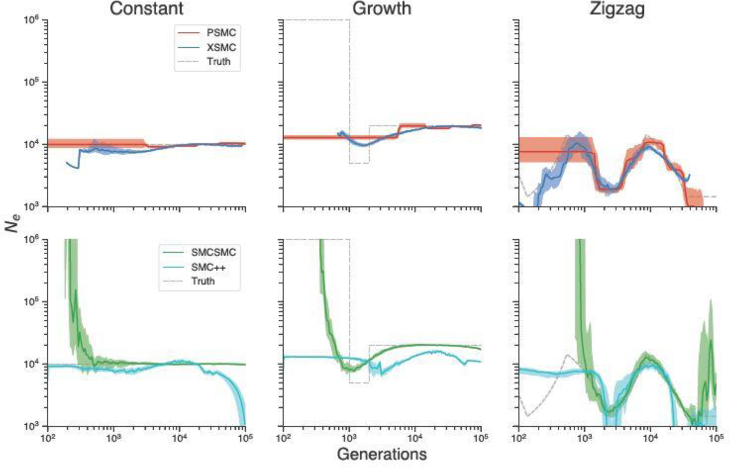
Comparison of XSMC, PSMC, SMCSMC, SMC++ on various simulated size histories.

The left column of the figure (“Constant”) depicts the most basic scenario, where the population size is unchanged over time. While all methods do an acceptable job, PSMC and XSMC exhibit less bias. For PSMC, there is some bias from the piecewise-constant model class it uses to perform estimation. (We note that with its default settings, PSMC actually initializes to the true model in this scenario.) XSMC has a slight downward bias in the recent past, but is otherwise centered over the true values $N_e={10}^4$. Both methods appear slightly biased in the period ${10}^3-{10}^4$ generations, though in opposite directions. SMCSMC performs well after ${10}^3$ about generations, however it incorrectly estimates a large increase in $N_e$ towards the present. SMC++ exhibits a slight downward bias towards the recent past and also incorrectly estimates a population crash further back in time.

In the center column (“Growth”), we simulated a cartoon model of recent expansion, in which the population experiences a brief bottleneck from 2,000–1,000 generations ago, before suddenly increasing in size by two hundredfold. This model is more difficult to correctly infer using only diploid data, because the large recent population size prevents samples from coalescing during this time, depriving methods of the ability to learn size history in the recent past. Nevertheless, XSMC does an acceptable job of showing that the population experienced a dip followed by a sharp increase, though the estimates are oversmoothed. In contrast, PSMC estimates size history that is nearly flat, with no acknowledgement of the bottleneck. SMC++ estimates a similar trajectory as XSMC, but is slightly more downward biased at all points in time. At an initial glance, SMCSMC looks to have most faithfully estimated the population size history. However, the results from the other two scenarios indicate that SMCSMC tends to infer a recent growth in population whether or not it actually occurred. Even so, without considering this feature of the model, SMCSMC returns a similar result to XSMC. This result also illustrates another benefit of the nonparametric approach: XSMC only returns an answer where it actually observes data. Because no coalescence times were observed before $~{10}^3$ generations when sampling from the posterior, our method does not plot anything outside of that region. This compares favorably with PSMC and related parametric methods (e.g., Schiffels and Durbin, 2014, Terhorst et al., 2017, Steinrücken et al., 2019), which have to model $N_e\left(t\right)$ over all $0\le t<\mathrm{\infty }$ in order to perform an analysis, even when the data contain no signal outside of a limited region.

Lastly, in the right-hand column we examined a difficult demography known in the literature as the zigzag model (Schiffels and Durbin, 2014). This is a pathological model of repeated exponential expansions and contractions, and is designed to benchmark various demographic inference procedures. We found that with the default setting $\rho =\theta$ used in the preceding two examples, the methods failed to produce good results on the zigzag. We therefore lowered the rate of recombination to $r={10}^{-9}$ /bp/generation in order to create more linkage disequilibrium for the methods to exploit. Here, a fairly substantial difference emerges between the two methods. XSMC does the best job of inferring this difficult size history, with accurate results to almost ${10}^2$ generations in the past, and almost no discernible bias. It is also the only method to successfully infer the final population crash in the recent past. In contrast, PSMC and SMC++ return similar results where the methods are able to recover the true value accurately after ${10}^3$ generations. SMCSMC also returns similar results to PSMC and SMC++, but again the method incorrectly infers a population increase both towards the present and further back in the past.

Table 3 displays the total running time in minutes of the four methods of the 75 total simulations across the three different demographies. Each method was parallelized across the simulations and run on a 32-core machine. XSMC and PSMC completed the simulations significantly faster than SMC++ and SMCSMC, and between the two methods, XSMC outperformed PSMC computationally by a relatively large margin. The simulation results show that XSMC can deliver high quality estimates of demography more quickly than competing methods.

Table 3.

Total running time of XSMC, PSMC, SMCSMC, and SMC++ in minutes of 75 total simulations on various simulated size histories.

Method	Minutes
SMC++	519.865721
SMCSMC	1840.547969
XSMC	0.891570
PSMC	1.401326

Encouraged by these results, we next turned to analyzing real data. We performed a simple analysis where we analyzed whole genome data from 20 individuals from each of the five superpopulations (African, European, East Asian, South Asian, and Admixed American) in the 1000 Genomes dataset (The 1000 Genomes Project Consortium, 2015). Results are shown in Figure 2. Broadly speaking, our method agrees with other recently-published estimates (Li and Durbin, 2011, Terhorst et al., 2017), and succeeds in capturing major recent events in human history such as an out-of-Africa event 100–200kya, a bottleneck experienced by non-African populations, and explosive recent growth beginning around 20kya. On the other hand, certain features that have been found in previous analyses (e.g. the peak and drop before 100Kya in Figure 3a of Li and Durbin, 2011) are smoothed out by our method, likely due to the novel use of kernel methods here. These estimates could probably be improved with fine-tuning and the use of additional data, but we did not attempt this, the message being that our method has moderate data requirements and produces reasonable results with minimal user intervention. Finally, we note that our method is highly efficient: to analyze all $20\times 5\times \left(3\times {10}^9\mathrm{\hspace{0.17em}M}\mathrm{b}\mathrm{p}\right)\approx 300\mathrm{G}\mathrm{b}\mathrm{p}$ of sequence data took approximately 40 minutes on a 12-core workstation. A single human genomes (all 22 autosomes) can be analyzed in about 30 seconds.

Fig. 2.

Result of fitting XSMC to 1000 Genomes data. For each superpopulation, 20 samples were chosen. Solid line denotes the median across all samples, and shaded bands denote the interquartile range.

4.4.2. Phasing and Imputation

The Li and Stephens (2003) haplotype copying model (hereafter, LS) is an approximation to the conditional distribution of a “focal” haplotype (e.g., a chromosome) given a set of other “panel” haplotypes. It supposes that the focal haplotype copies with error from different members of panel, occasionally switching to a new template due to recombination. Genealogically, this can be interpreted as finding the local genealogical nearest neighbor (GNN) of the focal haplotype within the panel. LS has been used extensively in applications, for example phasing diploid genotype data into haplotypes (Stephens and Scheet, 2005) and imputing missing data (Scheet and Stephens, 2006, Marchini et al., 2007, Howie et al., 2009). The method’s undeniable success is actually somewhat surprising, since it assumes an extremely simple genealogical relationship between the focal and panel haplotypes which ignores time completely (Paul and Song, 2010). Hence, while we motivated XSMC as a fast and slightly more approximate SMC prior, it can also be seen as a more biologically faithful version of LS.

We wondered whether our method could be used to improve downstream phasing and imputation. Fully implementing a phasing or imputation pipeline is beyond the scope of this paper, so we settled for checking in simulations whether decoding results produced by XSMC were more genealogically accurate than those obtained using LS. We simulated data using realistic models of human chromosomes 10 and 13 (Adrion et al., 2019). We chose these two because chromosome 10 is estimated to have an average ratio of recombination to mutation slightly above $1(\rho /\theta =1.07)$, while in chromosome 13 the ratio is slightly below $1(\rho /\theta =0.87)$. The ratio of recombination to mutation affects the difficulty of phasing and imputation, with higher ratios leading to less linkage disequilibrium and thus less accurate results. We also explored the effects of varying the size of the haplotype panel. For each chromosome, we simulated 10 data sets with panels of size $H=\mathrm{2,4},\mathrm{10,25,100}\mathrm{ }$.

As a proxy for phasing and imputation accuracy, we studied which method identified a genealogical nearer neighbor on average. The GNN at a given position is defined to be any panel haplotype that shares the earliest common ancestor with the focal haplotype. In other words, any panel haplotype that has the smallest TMRCA with the focal haplotype is a GNN. (Note that there may be more than one GNN.) For purposes of accurate phasing and imputation, it is desirable to identify the GNN as closely as possible.

For each simulation we computed the Viterbi path from XSMC and LS, as well as the posterior modal haplotype, and studied the proximity of those paths to the true GNN at each segregating site. Table S10 shows the proportion of segregating sites where XSMC and LS both estimated the same haplotype to be the GNN. For the MAP path, there is a high level of agreement, 80–90%, between the two methods for both small and large panel sizes. When the panel size is small $(H=2)$, there are few possible choices, and when the panel size is large $(H=100)$ the decoding consists mostly of long, recent stretches of IBD which are fairly easy to estimate. Disagreement is highest for intermediate values $H=4, 10, 25$ where neither of these effects dominates. At sample size $H=10$ the methods only agree at about half of segregating sites. The posterior mode appears to be less stable, with the agreement between the two methods decreasing monotonically as the panel size increases, down to agreement at only abouth 1/3rd of sites when $H=100$.

At the 10–66% of sites where the methods disagree, the results indicate a statistically significant gain for XSMC compared to LS. Table S11 shows that conditional on the two methods inferring different haplotypes as the GNN at that site, XSMC finds a genealogical nearer neighbor more often except in one case (chromosome 10, $H=10$, MAP path.) Using MAP estimation, the advantage of using XSMC increases, as the panel size increases, up to a roughly 6–10% advantage on chromosome $H=100$. For the posterior mode, the methods perform more comparably, and the largest difference is on the order of a few percentage points. The performance difference is significantly different from equal odds in almost every case.

5. Conclusion

In this article, we studied the sequentially Markov coalescent, a framework for approximating the likelihood of genetic data under various evolutionary models. We proposed a new inference method which supposes that the heights of neighboring identity-by-descent segments are independent. We showed that this led to decoding algorithms which are faster and have less bias than existing algorithms.

There are several possible extensions to our work. It is straightforward to extend our techniques to allow for position-specific rates of recombination and mutation, which could then be used to infer spatial or motif-specific variation in these processes.

Although we focused here on analyzing data from a single, panmictic population, we can also use posterior samples or MAP estimates to infer more complicated models of population structure. It is also possible to extend some of our techniques to other priors which model correlations between adjacent IBD segments. For the Viterbi decoder, we were able to implement a version of the algorithm in Section 3.3 which works for McVean and Cardin’s original SMC model. This could be useful, for example, if analyzing data from a structured population, to the extent that adjacent segments of identity by descent are more likely to derive from members of the same subpopulation. However, the resulting procedure is much more complicated. The Viterbi function $V_n\left(t\right)$ no longer has the tractable form derived in Proposition 3. Consequently, we cannot use a simple method like the one in Appendix S6 to perform the pointwise maximization in equation (4). Instead, numerical optimization must be used instead, resulting in a slower algorithm.

Another interesting possibility is to use our method to estimate ancestral recombination graphs. Recently, there has been a resurgence of interest in inferring ARGs using large samples of cosmopolitan genomic data (Kelleher et al., 2019, Speidel et al., 2019). Although these represent an impressive breakthrough, they rely on heuristic estimation procedures that do not directly model the underlying genealogical process that generates ancestry. Our method provides a new possibility for ARG estimation, by iteratively adding samples onto a sequence of estimated genealogies, but without the need to discretize those genealogies. These and other extensions are the subjects of ongoing work.

References

- Adrion JR, Cole CB, Dukler N, Galloway JG, Gladstein AL, Gower G, Kyriazis CC, Ragsdale AP, Tsambos G, Baumdicker F, Carlson J, Cartwright RA, Durvasula A, Kim BY, McKenzie P, Messer PW, Noskova E, Vecchyo DO-D, Racimo F, Struck TJ, Gravel S, Gutenkunst RN, Lohmeuller KE, Ralph PL, Schrider DR, Siepel A, Kelleher J, and Kern AD (2019), “A community-maintained standard library of population genetic models,” bioRxiv,. [DOI] [PMC free article] [PubMed] [Google Scholar]
- Barry D, and Hartigan JA (1992), “Product partition models for change point problems,” The Annals of Statistics, pp. 260–279. [Google Scholar]
- Barry D, and Hartigan JA (1993), “A Bayesian analysis for change point problems,” Journal of the American Statistical Association, 88(421), 309–319. [Google Scholar]
- Bhaskar A, Wang YXR, and Song YS (2015), “Efficient inference of population size histories and locus-specific mutation rates from large-sample genomic variation data,” Genome Research, 25(2), 268–279. [DOI] [PMC free article] [PubMed] [Google Scholar]
- Bishop CM (2006), Pattern Recognition and Machine Learning, Berlin, Heidelberg: Springer-Verlag. [Google Scholar]
- Carmi S, Wilton PR, Wakeley J, and Pe’er I (2014), “A renewal theory approach to IBD sharing,” Theoretical population biology, 97, 35–48. [DOI] [PMC free article] [PubMed] [Google Scholar]
- Chan AH, Jenkins PA, and Song YS (2012), “Genome-Wide Fine-Scale Recombination Rate Variation in Drosophila melanogaster,” PLoS Genetics, 8(12), e1003090. [DOI] [PMC free article] [PubMed] [Google Scholar]
- Chan NH, Ng WL, Yau CY, and Yu H (2021), “Optimal change-point estimation in time series,” The Annals of Statistics, 49(4), 2336–2355. [Google Scholar]
- Drummond AJ, Rambaut A, Shapiro B, and Pybus OG (2005), “Bayesian coalescent inference of past population dynamics from molecular sequences,” Molecular biology and evolution, 22(5), 1185–1192. [DOI] [PubMed] [Google Scholar]
- Durbin R (2014), “Efficient haplotype matching and storage using the positional Burrows-Wheeler transform (PBWT),” Bioinformatics, 30(9), 1266–1272. [DOI] [PMC free article] [PubMed] [Google Scholar]
- Durrett R (2008), Probability Models for DNA Sequence Evolution, 2nd edn Springer, New York. [Google Scholar]
- Fearnhead P (2006), “Exact and efficient Bayesian inference for multiple changepoint problems,” Statistics and computing, 16(2), 203–213. [Google Scholar]
- Fearnhead P, and Liu Z (2011), “Efficient Bayesian analysis of multiple changepoint models with dependence across segments,” Statistics and Computing, 21(2), 217–229. [Google Scholar]
- Gay JC, Myers S, and McVean G (2007), “Estimating meiotic gene conversion rates from population genetic data,” Genetics, 177, 881–894. [DOI] [PMC free article] [PubMed] [Google Scholar]
- Gill MS, Lemey P, Faria NR, Rambaut A, Shapiro B, and Suchard MA (2013), “Improving Bayesian population dynamics inference: a coalescent-based model for multiple loci,” Molecular biology and evolution, 30(3), 713–724. [DOI] [PMC free article] [PubMed] [Google Scholar]
- Griffiths RC, and Marjoram P (1997), “An ancestral recombination graph,” in Progress in population genetics and human evolution, eds. Donnelly P, and Tavaré S, Vol. 87 Springer-Verlag, Berlin, pp. 257–270. [Google Scholar]
- Griffiths R, and Marjoram P (1996), “Ancestral inference from samples of DNA sequences with recombination,” Journal of Computational Biology, 3(4), 479–502. [DOI] [PubMed] [Google Scholar]
- Gutenkunst RN, Hernandez RD, Williamson SH, and Bustamante CD (2009), “Inferring the Joint Demographic History of Multiple Populations from Multidimensional SNP Frequency Data,” PLoS Genetics, 5(10), e1000695. [DOI] [PMC free article] [PubMed] [Google Scholar]
- Harris K, Sheehan S, Kamm JA, and Song YS (2014), Decoding coalescent hidden Markov models in linear time,, in Proc. 18th Annual Intl. Conf. on Research in Computational Molecular Biology (RECOMB), Vol. 8394 of LNBI, Springer, pp. 100–114. (NIHMSID 597680, PMC Pending). [DOI] [PMC free article] [PubMed] [Google Scholar]
- Hein J, Schierup MH, and Wiuf C (2005), Gene genealogies, variation and evolution Oxford University Press. [Google Scholar]
- Henderson D, Zhu SJ, Cole CB, and Lunter G (2021), “Demographic inference from multiple whole genomes using a particle filter for continuous Markov jump processes,” PLoS One, 16(3), e0247647. [DOI] [PMC free article] [PubMed] [Google Scholar]
- Hobolth A, and Jensen JL (2014), “Markovian approximation to the finite loci coalescent with recombination along multiple sequences,” Theoretical population biology, 98, 48–58. [DOI] [PubMed] [Google Scholar]
- Howie B, Fuchsberger C, Stephens M, Marchini J, and Abecasis GR (2012), “Fast and accurate genotype imputation in genome-wide association studies through pre-phasing,” Nat. Genet, 44(8), 955–959. [DOI] [PMC free article] [PubMed] [Google Scholar]
- Howie BN, Donnelly P, and Marchini J (2009), “A flexible and accurate genotype imputation method for the next generation of genome-wide association studies,” PLoS Genet, 5(6), e1000529. [DOI] [PMC free article] [PubMed] [Google Scholar]
- Huang J, Howie B, McCarthy S, Memari Y, Walter K, Min JL, Danecek P, Malerba G, Trabetti E, Zheng H-F, UK10K Consortium, Gambaro G, Richards JB, Durbin R, Timpson NJ, Marchini J, and Soranzo N (2015), “Improved imputation of low-frequency and rare variants using the UK10K haplotype reference panel,” Nat. Commun, 6, 8111. [DOI] [PMC free article] [PubMed] [Google Scholar]
- Jackson B, Scargle JD, Barnes D, Arabhi S, Alt A, Gioumousis P, Gwin E, Sangtrakulcharoen P, Tan L, and Tsai TT (2005), “An algorithm for optimal partitioning of data on an interval,” IEEE Signal Processing Letters, 12(2), 105–108. [Google Scholar]
- Jouganous J, Long W, Ragsdale AP, and Gravel S (2017), “Inferring the Joint Demographic History of Multiple Populations: Beyond the Diffusion Approximation,” Genetics, 206(3), 1549–1567. [DOI] [PMC free article] [PubMed] [Google Scholar]
- Kamm JA, Terhorst J, and Song YS (2017), “Efficient computation of the joint sample frequency spectra for multiple populations,” J. Comput. Graph. Stat, 26(1), 182–194. [DOI] [PMC free article] [PubMed] [Google Scholar]
- Kamm J, Terhorst J, Durbin R, and Song YS (2020), “Efficiently inferring the demographic history of many populations with allele count data,” J. Am. Stat. Assoc, 115(531), 1472–1487. [DOI] [PMC free article] [PubMed] [Google Scholar]
- Kelleher J, Wong Y, Wohns AW, Fadil C, Albers PK, and McVean G (2019), “Inferring whole-genome histories in large population datasets,” Nature Genetics, 51(9), 1330–1338. [DOI] [PMC free article] [PubMed] [Google Scholar]
- Killick R, Fearnhead P, and Eckley IA (2012), “Optimal detection of changepoints with a linear computational cost,” Journal of the American Statistical Association, 107(500), 1590–1598. [Google Scholar]
- Lawson D, Hellenthal G, Myers S, and Falush D (2012), “Inference of Population Structure using Dense Haplotype Data,” PLoS Genetics, 8(1), e1002453. [DOI] [PMC free article] [PubMed] [Google Scholar]
- Lember J, and Koloydenko AA (2014), “Bridging Viterbi and posterior decoding: a generalized risk approach to hidden path inference based on hidden Markov models, “ The Journal of Machine Learning Research, 15(1), 1–58. [Google Scholar]
- Li H, and Durbin R (2011), “Inference of human population history from individual whole-genome sequences,” Nature, 475, 493–496. [DOI] [PMC free article] [PubMed] [Google Scholar]
- Li N, and Stephens M (2003), “Modeling Linkage Disequilibrium and Identifying Recombination Hotspots Using Single-Nucleotide Polymorphism Data,” Genetics, 165, 2213–2233. [DOI] [PMC free article] [PubMed] [Google Scholar]
- Lunter G (2019), “Haplotype matching in large cohorts using the Li and Stephens model,” Bioinformatics, 35(5), 798–806. [DOI] [PMC free article] [PubMed] [Google Scholar]
- Marchini J, Howie B, Myers SR, McVean G, and Donnelly P (2007), “A new multipoint method for genome-wide association studies by imputation of genotypes,” Nat Genet, 39(7), 906–13. [DOI] [PubMed] [Google Scholar]
- Marjoram P, and Wall JD (2006), “Fast “coalescent” simulation,” BMC Genet, 7,16. [DOI] [PMC free article] [PubMed] [Google Scholar]
- McVean GA, and Cardin NJ (2005), “Approximating the coalescent with recombination,” Philosophical Transactions of the Royal Society B: Biological Sciences, 360(1459), 1387–1393. [DOI] [PMC free article] [PubMed] [Google Scholar]
- Minin VN, Bloomquist EW, and Suchard MA (2008), “Smooth skyride through a rough skyline: Bayesian coalescent-based inference of population dynamics,” Molecular biology and evolution, 25(7), 1459–1471. [DOI] [PMC free article] [PubMed] [Google Scholar]
- Palamara PF, Terhorst J, Song YS, and Price AL (2018), “High-throughput inference of pairwise coalescence times identifies signals of selection and enriched disease heritability,” Nature Genetics, 50(9), 1311–1317. [DOI] [PMC free article] [PubMed] [Google Scholar]
- Parag KV, and Pybus OG (2019), “Robust design for coalescent model inference,” Systematic biology, 68(5), 730–743. [DOI] [PubMed] [Google Scholar]
- Paul JS, and Song YS (2010), “A Principled Approach to Deriving Approximate Conditional Sampling Distributions in Population Genetics Models with Recombination,” Genetics, 186, 321–338. [DOI] [PMC free article] [PubMed] [Google Scholar]
- Paul JS, Steinrücken M, and Song YS (2011), “An accurate sequentially Markov conditional sampling distribution for the coalescent with recombination,” Genetics, 187, 1115–1128. (PMC3070520). [DOI] [PMC free article] [PubMed] [Google Scholar]
- Price AL, Tandon A, Patterson N, Barnes KC, Rafaels N, Ruczinski I, Beaty TH, Mathias R, Reich D, and Myers SR (2009), “Sensitive detection of chromosomal segments of distinct ancestry in admixed populations,” PLoS Genet, 5(6), e1000519. [DOI] [PMC free article] [PubMed] [Google Scholar]
- Pybus OG, Rambaut A, and Harvey PH (2000), “An integrated framework for the inference of viral population history from reconstructed genealogies,” Genetics, 155(3), 1429–1437. [DOI] [PMC free article] [PubMed] [Google Scholar]
- Rasmussen MD, Hubisz MJ, Gronau I, and Siepel A (2014), “Genome-wide inference of ancestral recombination graphs,” PLoS Genetics, 10(5), e1004342. [DOI] [PMC free article] [PubMed] [Google Scholar]
- Rubinacci S, Ribeiro DM, Hofmeister RJ, and Delaneau O (2021), “Efficient phasing and imputation of low-coverage sequencing data using large reference panels,” Nat. Genet, 53(1), 120–126. [DOI] [PubMed] [Google Scholar]
- Scheet P, and Stephens M (2006), “A fast and flexible statistical model for large-scale population genotype data: Applications to inferring missing genotypes and haplotypic phase,” Am. J. Hum. Genet, 78, 629–644. [DOI] [PMC free article] [PubMed] [Google Scholar]
- Schiffels S, and Durbin R (2014), “Inferring human population size and separation history from multiple genome sequences,” Nature Genetics, 46, 919–925. [DOI] [PMC free article] [PubMed] [Google Scholar]
- Sheehan S, Harris K, and Song YS (2013), “Estimating variable effective population sizes from multiple genomes: A sequentially Markov conditional sampling distribution approach,” Genetics, 194(3), 647–662. [DOI] [PMC free article] [PubMed] [Google Scholar]
- Shi X, Gallagher C, Lund R, and Killick R (2022), “A comparison of single and multiple changepoint techniques for time series data,” Comput. Stat. Data Anal, 170, 107433. [Google Scholar]
- Speidel L, Forest M, Shi S, and Myers SR (2019), “A method for genome-wide genealogy estimation for thousands of samples,” Nature Genetics, 51(9), 1321–1329. [DOI] [PMC free article] [PubMed] [Google Scholar]
- Spence JP, Steinrücken M, Terhorst J, and Song YS (2018), “Inference of population history using coalescent HMMs: Review and outlook,” Current opinion in genetics & development, 53, 70–76. [DOI] [PMC free article] [PubMed] [Google Scholar]
- Steinrücken M, Kamm J, Spence JP, and Song YS (2019), “Inference of complex population histories using whole-genome sequences from multiple populations,” Proceedings of the National Academy of Sciences, 116(34), 17115–17120. [DOI] [PMC free article] [PubMed] [Google Scholar]
- Stephens M, and Scheet P (2005), “Accounting for decay of linkage disequilibrium in haplotype inference and missing-data imputation,” Am. J. Hum. Genet, 76(3), 449–62. [DOI] [PMC free article] [PubMed] [Google Scholar]
- Terhorst J, Kamm JA, and Song YS (2017), “Robust and scalable inference of population history from hundreds of unphased whole genomes,” Nature genetics, 49(2), 303–309. [DOI] [PMC free article] [PubMed] [Google Scholar]
- The 1000 Genomes Project Consortium (2015), “A global reference for human genetic variation,” Nature, 526(7571), 68–74. [DOI] [PMC free article] [PubMed] [Google Scholar]
- Voight BF, Kudaravalli S, Wen X, and Pritchard JK (2006), “A Map of Recent Positive Selection in the Human Genome,” PLoS Biology, 4, e72. [DOI] [PMC free article] [PubMed] [Google Scholar]
- Wang J-L (2014), “Smoothing hazard rates,” Wiley StatsRef: Statistics Reference Online,. [Google Scholar]
- Wiuf C, and Hein J (1999), “Recombination as a point process along sequences,” Theor. Popul. Biol, 55, 248–259. [DOI] [PubMed] [Google Scholar]
- Yau C, and Holmes CC (2013), “A decision-theoretic approach for segmental classification,” The Annals of Applied Statistics, pp. 1814–1835. [Google Scholar]
Associated Data
This section collects any data citations, data availability statements, or supplementary materials included in this article.