Diffuse optical tomography of the brain: effects of inaccurate baseline optical parameters and refinements using learned post-processing

Abstract

Diffuse optical tomography (DOT) uses near-infrared light to image spatially varying optical parameters in biological tissues. In functional brain imaging, DOT uses a perturbation model to estimate the changes in optical parameters, corresponding to changes in measured data due to brain activity. The perturbation model typically uses approximate baseline optical parameters of the different brain compartments, since the actual baseline optical parameters are unknown. We simulated the effects of these approximate baseline optical parameters using parameter variations earlier reported in literature, and brain atlases from four adult subjects. We report the errors in estimated activation contrast, localization, and area when incorrect baseline values were used. Further, we developed a post-processing technique based on deep learning methods that can reduce the effects due to inaccurate baseline optical parameters. The method improved imaging of brain activation changes in the presence of such errors.

1. Introduction

Diffuse optical tomography (DOT) is a non-invasive technique for imaging spatially varying optical parameters in biological tissues [1–3]. The distribution of these optical parameters provides tissue biochemical and structural information with applications in early diagnosis and imaging of breast cancer, monitoring neonatal brains, and preclinical imaging of small animals [2,4]. Brain activity increases local blood flow, which can be localized using DOT to study task-evoked and resting-state networks in the brain [5,6]. In general, DOT is non-ionizing and non-invasive, and its instrumentation is relatively simple, low-cost, and portable, compared to conventional medical tomographic techniques [6].

Nevertheless, the image reconstruction problem in DOT is ill posed. The ill-posedness means that even small errors in measurements or modeling can cause large errors in the reconstructions [1]. Furthermore, DOT of the human adult brain is challenging due to light attenuation by the thick scattering skull, and the lateral spreading of light by the low-scattering cerebro-spinal fluid (CSF) layer, restricting light penetration into the gray and white matter [6,7]. A subject-specific model of the different brain compartments obtained using magnetic resonance imaging (MRI) or computed tomography (CT) has been shown to significantly improve the DOT image reconstruction [8,9]. In the absence of such complementary information, fitting a general head template to the location of optodes and other fiducial points has also shown promising improvements [10,11]. As regards to the modeling of light transport in the brain, the radiative transport equation (RTE) is the most accurate model and its solution can be obtained using Monte Carlo simulations [12]. Hybrid modeling techniques utilising the RTE for the low-diffusive CSF region and a diffusion approximation for the diffusive scalp, skull, and brain tissue regions, have also been proposed [13–15]. Nevertheless, since the CSF region is relatively thin and highly convoluted, it has been demonstrated that the diffusion approximation can be used as a reasonable model for the image reconstruction [16,17]. Apart from these, earlier research has also addressed the problems of removing interference by superficial physiological processes (pulse, respiration, and blood pressure oscillations) from brain activity [18,19], calibration of optode positions on the brain [20], and marginalizing errors due to unknown shape of the brain [21].

Recently, deep learning methods have shifted the focus of tomographic techniques from purely model-based techniques to data-driven approaches [22–24]. Initial deep learning methods in DOT directly learned the non-linear mapping of the surface measurements to the spatially distributed optical coefficients, utilising classical or convolutional neural networks (CNNs) [25–27]. More recently, model-based learning approaches that combine deep learning with classical model equations have been proposed in DOT [28–30]. Model-based learning can overcome some inherent limitations of the pure learning approaches, such as biases due to training samples and requirements of large training datasets [31–33]. These computational developments have progressed with improvements in experimental brain imaging systems, that use novel spatial, temporal, and frequency encoding strategies [6]. For more information on DOT of the brain and related methodologies, see e.g. [2,4–6].

DOT functional brain imaging utilises a perturbation model where changes in measured signals due to brain activity, are considered as a linear function of the changes in the optical parameters [6]. The perturbation model utilises baseline optical parameters of the human brain, to estimate the optical parameter changes. Since the actual baseline optical parameters are unknown, those are usually based on literature-reported values [6,10]. However, this procedure can lead to errors as the baseline optical parameters of the human brain have been shown to vary extensively across different subjects [34,35]. For example, the results presented by Choi et al. [34] show that the optical parameters in the adult brain (20 to 50 years) vary around 20% from the cross-subject average values. Farina et al. [35] reported up to 50% inter-subject variations in optical parameters, including variations due to the use of different types of optical instruments. These large variations can also be noted in the reported optical properties of the brain in other studies [36–38]. The effects of unknown baseline optical parameters in DOT of the neonatal brain were simulated by Heiskala et al. [39] using one neonatal brain atlas. The study reported errors in peak contrast and localization when erroneous baseline optical parameters were used in the image reconstruction. To our knowledge, the impact of unknown baseline optical parameters in adult brain imaging and methods to alleviate such errors has not been reported yet. Since the DOT image reconstruction is highly ill posed, the effect of these errors could be significant [39]. As it is practically infeasible to obtain the actual optical parameter distributions of an adult brain, an alternative is to carry out simulations with realistic brain atlases.

In this work, we study and report the errors due to the use of inaccurate baseline optical parameters in DOT using brain atlases from four adult subjects. Further, we follow the model-based learning approach to develop a post-processing technique that can marginalize the resulting errors. The remainder of the paper is organized as follows. In Section 2, we review the light transport model, the conventional image reconstruction model, and describe our proposed post-processing technique. Simulations are described in Section 3. Results are presented in Section 4. Finally, the conclusions are given in Section 6.

2. Methods

2.1. Diffuse optical tomography

In a DOT measurement setup, near-infrared light is introduced into an object from its boundary. Let $\mathrm{\Omega }\subset {\mathbb{R}}^3$ denote the three-dimensional object domain with boundary $\mathrm{\partial }\mathrm{\Omega }$ . A commonly used light transport model for DOT is the diffusion approximation to the radiative transfer equation [40]. Here, we consider the steady-state version of the diffusion approximation [1,41]

$$-\mathrm{\nabla }\cdot \frac{1}{3({\mu }_{\text{a}}(r)+{\mu }_{\text{s}}^{\prime }(r))}\mathrm{\nabla }\mathrm{\Phi }(r)+{\mu }_{\text{a}}(r)\mathrm{\Phi }(r)=0,r\in \mathrm{\Omega },$$ (1)

$$\mathrm{\Phi }(r)+\frac{1}{3({\mu }_{\text{a}}(r)+{\mu }_{\text{s}}^{\prime }(r))}\alpha \frac{\mathrm{\partial }\mathrm{\Phi }(r)}{\mathrm{\partial }\hat{n}}=\{\begin{array}{cc}q,& r\in s\\ 0,& r\in \mathrm{\partial }\mathrm{\Omega }\setminus s\end{array},$$ (2)

where $\mathrm{\Phi }(r)$ is the photon fluence, ${\mu }_{\text{a}}(r)$ is the absorption coefficient and ${\mu }_{\text{s}}^{\prime }(r)$ is the (reduced) scattering coefficient. The reduced scattering coefficient is a property incorporating the scattering coefficient ${\mu }_{\mathrm{s}}$ and the scattering anisotropy $-1<g<1$ , given by ${\mu }_{\text{s}}^{\prime }={\mu }_{\mathrm{s}}(1-g)$ . The parameter $q$ is the strength of the continuous-wave light source at location $s\subset \mathrm{\partial }\mathrm{\Omega }$ . Further, $\alpha$ is a function of the effective reflection coefficient owing to Fresnel reflection at the boundary $\mathrm{\partial }\mathrm{\Omega }$ , and $\hat{n}$ is an outward unit vector normal to the boundary. The measurable data on the boundary of the object, exitance $\gamma (r)$ , is given by

$$\gamma (r)=-\frac{1}{3({\mu }_{\text{a}}(r)+{\mu }_{\text{s}}^{\prime }(r))}\frac{\mathrm{\partial }\mathrm{\Phi }(r)}{\mathrm{\partial }\hat{n}}=\frac{1}{\alpha }\mathrm{\Phi }(r).$$ (3)

The numerical approximation of the forward model (1)–(3) is typically based on a finite element (FE) approximation [1]. In the FE-approximation, the domain $\mathrm{\Omega }$ is divided into ${\mathrm{N}}_{\mathrm{e}}$ non-overlapping elements joined at ${\mathrm{N}}_{\mathrm{n}}$ vertex nodes. We write the finite-dimensional approximations for $\mathrm{\Phi }(r)$ , ${\mu }_{\text{a}}(r)$ and ${\mu }_{\text{s}}^{\prime }(r)$ as

$$\mathrm{\Phi }(r)\approx \sum _{k=1}^{{\text{N}}_{\mathrm{n}}}{\varphi }_k{\psi }_k(r),{\mu }_{\mathrm{a}}(r)\approx \sum _{k=1}^{{\text{N}}_{\mathrm{n}}}{\mu }_{\text{a},k}{\psi }_k(r),{\mu }_{\text{s}}^{\prime }(r)\approx \sum _{k=1}^{{\text{N}}_{\mathrm{n}}}{\mu }_{\text{s},k}^{\prime }{\psi }_k(r),$$ (4)

where ${\psi }_k$ are the nodal basis functions of the FE-mesh, ${\varphi }_k$ is photon fluence and ${\mu }_{\text{a},k}$ , ${\mu }_{\text{s},k}^{\prime }$ denote the absorption and scattering at the nodes of the FE-discretisation. In this work, the FE-approximation was utilized with the Galerkin formulation [42].

A typical data type for continuous-wave DOT is the logarithm of amplitude, which is obtained from the logarithm of exitance, as

$$y=\log (\gamma ),$$ (5)

where $y\in {\mathbb{R}}^{{\mathrm{N}}_{\mathrm{m}}}$ is the data vector, and ${\mathrm{N}}_{\mathrm{m}}$ is the number of measurements. The FE-approximation of (1)–(3) is denoted by operator $A$ and the observation model is written as

$$y=A({\mu }_{\text{a}},{\mu }_{\text{s}}^{\prime })+e,$$ (6)

where $e\in {\mathbb{R}}^{{\mathrm{N}}_{\mathrm{m}}}$ models the random noise in measurements, ${\mu }_{\text{a}}=[{\mu }_{\mathrm{a},1},\dots ,{\mu }_{\mathrm{a},{\mathrm{N}}_{\mathrm{n}}}]\in {\mathbb{R}}^{{\mathrm{N}}_{\mathrm{n}}}$ and ${\mu }_{\text{s}}^{\prime }=[{\mu }_{\mathrm{s},1}^{\prime },\dots ,{\mu }_{\mathrm{s},{\mathrm{N}}_{\mathrm{n}}}^{\prime }]\in {\mathbb{R}}^{{\mathrm{N}}_{\mathrm{n}}}$ are discretized absorption and scattering coefficients.

2.2. Conventional difference imaging

Functional DOT brain imaging utilizes changes in the measurements due to corresponding changes in brain absorption, to monitor cerebral haemodynamics [6,10]. Consider data $y_1$ and $y_2$ of two log-intensity measurements obtained from a target with optical parameters at two different time instances as ( ${\mu }_{\text{a},1},{\mu }_{\text{s},1}^{\prime }$ ) and ( ${\mu }_{\text{a},2},{\mu }_{\text{s},2}^{\prime })$ , respectively. These two measurements are represented by the model, Eq. (6) as

$$y_1=A({\mu }_{\text{a},1},{\mu }_{\text{s},1}^{\prime })+e_1,$$ (7)

$$y_2=A({\mu }_{\text{a},2},{\mu }_{\text{s},2}^{\prime })+e_2.$$ (8)

Considering the change in measurements is purely due to the change in absorption ( ${\mu }_{\text{s},2}^{\prime }={\mu }_{\text{s},1}^{\prime }$ ), the change in measurements $\delta y=y_2-y_1$ , due to the change in absorption $\delta {\mu }_{\text{a}}$ = ${\mu }_{\text{a},2}-{\mu }_{\text{a},1}$ , is given by the linear perturbation model [6,10]

$$\delta y=J\delta {\mu }_{\text{a}}+\delta e$$ (9)

where the change in absorption $\delta {\mu }_{\text{a}}$ = ${\mu }_{\text{a},2}-{\mu }_{\text{a},1}$ , and Jacobian $J=\frac{\mathrm{\partial }A}{\mathrm{\partial }{\mu }_{\text{a}}}$ is the discrete representation of the Fréchet derivative of the nonlinear operator $A$ , evaluated at the baseline (or initial) optical parameters $({\mu }_{\text{a},1},{\mu }_{\text{s},1}^{\prime })$ . Here, $\delta e=e_2-e_1$ is the error, or noise in the difference measurements. Considering Gaussian distributed absorption parameter changes and noise

$$\delta {\mu }_{\text{a}}\sim \mathcal{N}(0,{\mathrm{\Gamma }}_{\delta {\mu }_{\mathrm{a}}}),\delta e\sim \mathcal{N}(0,{\mathrm{\Gamma }}_{\delta e}),$$

where ${\mathrm{\Gamma }}_{\delta {\mu }_{\mathrm{a}}}$ is the prior covariance and ${\mathrm{\Gamma }}_{\delta e}$ is the noise covariance, the maximum a posteriori (MAP) estimate for difference imaging is given by the following closed-form expression

$$\delta {\mu }_{\mathrm{a}}^{\mathrm{r}\mathrm{e}\mathrm{c}\mathrm{o}\mathrm{n}}=\underset{\delta {\mu }_{\text{a}}}{\arg min}\Vert \delta y-J\delta {\mu }_{\text{a}}{\Vert }_{{\mathrm{\Gamma }}_{\delta e}^{-1}}^2+\Vert \delta {\mu }_{\text{a}}{\Vert }_{{\mathrm{\Gamma }}_{\delta {\mu }_a}^{-1}}^2={(J^{\mathrm{T}}{\mathrm{\Gamma }}_{\delta e}^{-1}J+{\mathrm{\Gamma }}_{\delta {\mu }_{\text{a}}}^{-1})}^{-1}\cdot \left(J^{\mathrm{T}}{\mathrm{\Gamma }}_{\delta e}^{-1}\delta y\right).$$ (10)

When considering the difference data $\delta y$ , at least part of the systematic errors in the models/measurements are subtracted. However, the approach is based on the global linearisation of the non-linear observation model (6), which can lead to images that are qualitative and/or with weak spatial resolution [43]. Moreover, the estimates depend on the selection of the baseline optical parameters $({\mu }_{\text{a},1},{\mu }_{\text{s},1}^{\prime })$ , used in computing the Jacobian $J$ . Typically, the baseline parameters $({\mu }_{\text{a},1},{\mu }_{\text{s},1}^{\prime })$ for the different tissue compartments are based on previous findings [6,10]. This choice can lead to errors if the actual parameters differ from the assumed parameters.

2.3. Learned post-processing of the estimated images

In this work, we have developed a post-processing technique to improve the conventional estimate of optical parameters (10), in presence of erroneous baseline optical parameters $({\mu }_{\text{a},1},{\mu }_{\text{s},1}^{\prime })$ . For this, we extend a model-based iterative learning approach that we earlier proposed for absolute imaging [30] to the difference imaging problem. In this approach, we aim to learn an update function for the ‘model-based’ estimates (10) as

$$\delta {\mu }_{\mathrm{a}}^{\mathrm{p}\mathrm{o}\mathrm{s}\mathrm{t}}=G_{\theta }(\delta {\mu }_{\mathrm{a}}^{\mathrm{r}\mathrm{e}\mathrm{c}\mathrm{o}\mathrm{n}})$$ (11)

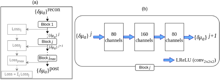
The update function $G_{\theta }$ corresponds to a CNN with network parameters $\theta$ learned from a set of training data. The function $G_{\theta }$ uses sequential CNN blocks as shown in Fig. 1. We have considered five blocks of CNNs, i.e., $j_{\mathrm{m}\mathrm{a}\mathrm{x}}=5$ . As shown in Fig. 1, the estimated absorption coefficients are given as an input to a pipeline. In each CNN block, the images are expanded to 80 and then 160 channels by a convolutional layer with kernel size of 2 pixels, and dimension $3$ , including bias and equipped with a ‘leaky’ rectified linear unit (LReLU) as non-linearity, that was defined for an input image $\mu$ as

$$\mathrm{L}\mathrm{R}\mathrm{e}\mathrm{L}\mathrm{U}(\mu )=\mathrm{m}\mathrm{a}\mathrm{x}(\mu ,0.1\mu ).$$

Fig. 1.

(a) Diagram of the CNN used to post-process the reconstructed absorption images ( ${\mu }_{\mathrm{a}}^{\mathrm{r}\mathrm{e}\mathrm{c}\mathrm{o}\mathrm{n}}$ ) consisting of processing blocks $1,\dots .,j_{\mathrm{m}\mathrm{a}\mathrm{x}}$ . (b) The structure of a processing block is shown. Here, the blue arrows denote a convolutional layer with 2 $\times$ 2 $\times$ 2 kernel for a 3D image, bias and followed by a LReLU. The resulting channels in each layer are indicated in the squares.

The expansive part of the network serves as a feature extractor (encoder) and the contracting part feature fusion (decoder).

The network was trained by simulations utilising a set of absorption and scattering distributions, i.e. ‘ground-truth images’ $\{{\mu }_{\mathrm{a},1}^{\mathrm{t}\mathrm{r}\mathrm{u}\mathrm{e}},{\mu }_{\mathrm{s},1}^{\prime \mathrm{t}\mathrm{r}\mathrm{u}\mathrm{e}},\delta {\mu }_{\mathrm{a}}^{\mathrm{t}\mathrm{r}\mathrm{u}\mathrm{e}}{\}}^i,i=1,\dots ,{\mathrm{N}}_{\mathrm{s}\mathrm{a}\mathrm{m}\mathrm{p}}$ . For these sample distributions, measurement data with change in absorption were computed using Eqs. (7), (8). Thereafter, the conventional difference estimates $\{\delta {\mu }_{\mathrm{a}}^{\mathrm{r}\mathrm{e}\mathrm{c}\mathrm{o}\mathrm{n}}{\}}^i$ were computed using Eq. (10), using the difference data $\delta y$ and incorrect values of baseline optical parameters. Meaning that, the difference estimates (10) were computed with a Jacobian matrix $J$ that was computed with incorrect baseline optical coefficients. The subsequent operation by the post-processing network (11) was to correct the errors in the estimated images caused by the incorrect baseline optical parameters. For this, the network parameters were trained by minimizing a ‘ ${\mathrm{L}}_2$ -loss’ cost function. The cost function for $i$ ’th sample and $j$ ’th CNN block was

$${\mathrm{C}\mathrm{o}\mathrm{s}\mathrm{t}}_j=\underset{{\theta }_j}{min}\sum _i\Vert G_{{\theta }_j}{(\{\delta {\mu }_{\mathrm{a}}{\}}^j)}^i-\{\delta {\mu }_{\mathrm{a}}^{\mathrm{t}\mathrm{r}\mathrm{u}\mathrm{e}}{\}}^i\Vert ,i=1,\dots ,{\mathrm{N}}_{\mathrm{s}\mathrm{a}\mathrm{m}\mathrm{p}}$$ (12)

The minimisation of the total cost from all the CNN blocks (Cost = $\sum _j{\mathrm{C}\mathrm{o}\mathrm{s}\mathrm{t}}_j$ ), as shown in Fig. 1 reduce the artifacts in the post-processed image by training the network parameters $\theta =\{{\theta }_j{\}}_{j=1\dots j_{\mathrm{m}\mathrm{a}\mathrm{x}}}$ . Requiring local optimality by (12), instead of only a final loss function for $\{\delta {\mu }_{\mathrm{a}}{\}}^{j_{\mathrm{m}\mathrm{a}\mathrm{x}}}$ , showed to reduce artifacts and improved training stability of the model.

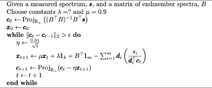
Training of the $\theta$ ’s was carried out by minimising (12) with the TensorFlow’s implementation of the Adam optimiser [44] using ${\mathrm{N}}_{\mathrm{s}\mathrm{a}\mathrm{m}\mathrm{p}}=2000$ , with batches of size 2, using 20 epochs and step size of ${10}^{-3}$ (learning rate). Since CNNs operate on uniform pixel domains, the ground-truth and reconstructed images in the mesh basis were interpolated to the image basis of size 25 $\times$ 25 $\times$ 25 for the application of the CNN. An application on meshes would be possible by using graph convolution [45,46]. The procedure for training the CNNs and obtaining the post-processed image ${\mu }_{\mathrm{a}}^{\mathrm{p}\mathrm{o}\mathrm{s}\mathrm{t}}$ , is summarised below in Algorithm 1.

Algorithm 1. Training the post-processing step.

2.4. Evaluating the post-processing step

After training the parameter sets $\theta$ ’s, the post-processing scheme was evaluated for a separate set of evaluation images $\{{\mu }_{\mathrm{a},1}^{\mathrm{t}\mathrm{r}\mathrm{u}\mathrm{e}},{\mu }_{\mathrm{s},1}^{\prime \mathrm{t}\mathrm{r}\mathrm{u}\mathrm{e}},\delta {\mu }_{\mathrm{a}}^{\mathrm{t}\mathrm{r}\mathrm{u}\mathrm{e}}{\}}^i,i=1,\dots ,{\mathrm{N}}_{\mathrm{e}\mathrm{v}\mathrm{a}\mathrm{l}}$ by applying the trained post-processing network $G_{\theta }$ . This procedure was equivalent to Algorithm 1, starting by drawing ${\mathrm{N}}_{\mathrm{e}\mathrm{v}\mathrm{a}\mathrm{l}}$ evaluation sets, computing the measurement data $\delta y$ and corresponding $\delta {\mu }_{\mathrm{a}}^{\mathrm{r}\mathrm{e}\mathrm{c}\mathrm{o}\mathrm{n}}$ , skipping the function ‘TRAIN’ and computing the post-processed image ${\mu }_{\mathrm{a}}^{\mathrm{p}\mathrm{o}\mathrm{s}\mathrm{t}}$ using the trained network $G_{\theta }$ . In this work, we evaluated the networks using ${\mathrm{N}}_{\mathrm{e}\mathrm{v}\mathrm{a}\mathrm{l}}=400$ samples using four different measurement domains. Details of these measurement domains are mentioned below in Section 3.1.

3. Simulations

The Toast++ software [47] was utilised in the FE-solution of the diffusion equation using MATLAB (R2017b, Mathworks, Natick, MA). A Python library, Tensorflow (version 2.10) [48] was utilised in implementation and training of the CNNs. The simulations, were carried out in a Fujitsu Celcius W550 desktop workstation, with IntelXeon W-2125 CPU @ 4.00GHz $\times$ 8cores, and operating system Ubuntu 22.04.2. The training of the CNNs was carried out on an NVIDIA Volta V100 GPU (Tesla V100-SXM2-32GB) with 1290MHz frequency, and operating system Red Hat Enterprise Linux, version 8.6.

3.1. Data generation

In our numerical studies, the domains $\mathrm{\Omega }\subset {\mathbb{R}}^3$ were four brain models from the open-source brain mesh library [49]. Subjects numbers 4, 18, 41, 54 of the library, which visually demonstrated the most significant structural differences, were chosen in this work. These subjects were normal adults with an age range of 24–37 years [50]. We refer to these four subjects as Subjects 1-4 and show the finite-element meshes of their brain atlases below in Fig. 2(a)-(d).

Fig. 2.

Finite-element meshes of the four adult subject brain atlases used in the study. The meshes are displayed to reveal the inner compartments of scalp (skin color), skull (white), CSF (blue) and grey matter (grey). Axes units are in mm.

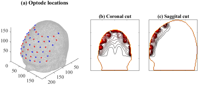
The measurement setup consisted of $27$ sources and $31$ detectors modelled as Gaussian surface patches of $2\mathrm{m}\mathrm{m}$ width located in interlaced fashion on the boundary, as shown in Fig. 3(a). Since the sources and detectors were located on the forehead, the brain regions with highest sensitivities to DOT imaging are immediately below the forehead, as shown in Fig. 3(b),(c). The baseline optical parameters of the different brain regions, with which parameter variations were studied are shown in Table 1. The measurement data sets $y_1$ and $y_2$ were simulated using the FE-approximation of the diffusion approximation (7), (8).

Fig. 3.

(a) Location of sources and detectors on the brain mesh of subject 1. The resulting sensitivity (Jacobian) values due to all sources and detectors were added and shown as contour plots along the (b) coronal and (c) sagittal plane of the domain.

Table 1. Optical parameters of the brain compartments chosen in this study, based on Refs. [51,52]. White matter (WM) and gray matter (GM) were chosen to have the same values. Units are in ${\mathrm{mm}}^{-1}$ .

Scalp		Skull		CSF		WM+GM
${\mu }_{\text{a}}$	${\mu }_{\text{s}}^{\prime }$	${\mu }_{\text{a}}$	${\mu }_{\text{s}}^{\prime }$	${\mu }_{\text{a}}$	${\mu }_{\text{s}}^{\prime }$	${\mu }_{\text{a}}$	${\mu }_{\text{s}}^{\prime }$
0.0191	0.66	0.0136	0.86	0.0026	0.01	0.0186	1.10

3.2. Noise model

We considered photon shot noise and dark current noise, since realistic modeling of the physiological noise remains a challenge. Dark current arises at the detectors even when no photons are detected. The current amplitude ( $A_{\mathrm{D}\mathrm{C}}$ ) can be measured when all light sources are off and it can be converted to an equivalent input optical noise equivalent power (NEP) at a certain bandwidth (BW) in units [W/ $\sqrt{\mathrm{H}\mathrm{z}}$ ] using the known responsivity ( $R$ ) in [A/W] of the detector [53,54], defined as

$$R=\frac{\eta e}{E_{\lambda }},$$ (13)

where $\eta$ is the quantum efficiency of the detector, $e$ is the elementary charge, and $E_{\lambda }$ is the energy of a photon at the selected wave length $\lambda$ [55]. The corresponding noise equivalent power for the selected source-wise single measurement time $t$ and BW ( $\mathrm{B}\mathrm{W}=1/(2t)$ ) is [53–55]

$$P_{\mathrm{N}\mathrm{E}\mathrm{P}}=\mathrm{N}\mathrm{E}\mathrm{P}\cdot \sqrt{\mathrm{B}\mathrm{W}}=\frac{A_{\mathrm{D}\mathrm{C}}}{R}.$$ (14)

This gives the dark current amplitude at the detector as

$$A_{\mathrm{D}\mathrm{C}}=\frac{\eta e{P}_{\mathrm{N}\mathrm{E}\mathrm{P}}}{E_{\lambda }}.$$

The corresponding mean current $(X_{\mathrm{D}\mathrm{C}})$ can be computed by setting to zero the detected photon current $X_{\mathrm{p}\mathrm{h}\mathrm{o}\mathrm{t}\mathrm{o}\mathrm{n}}$ in the definition of the total shot noise amplitude for a simple photodiode, without gain and shot noise dominating over thermal noise [55–57]

$$A_{\mathrm{t}\mathrm{o}\mathrm{t}\mathrm{a}\mathrm{l}\mathrm{n}\mathrm{o}\mathrm{i}\mathrm{s}\mathrm{e}}=\sqrt{2e(X_{\mathrm{p}\mathrm{h}\mathrm{o}\mathrm{t}\mathrm{o}\mathrm{n}}+X_{\mathrm{D}\mathrm{C}})\mathrm{B}\mathrm{W}}.$$ (15)

We get (see Eq. (3) in [58]; compare to first part of Eq. (12) in [59])

$$X_{\mathrm{D}\mathrm{C}}=\frac{{A_{\mathrm{D}\mathrm{C}}}^2}{2e\mathrm{B}\mathrm{W}}=\frac{{\eta }^2{e}^2{P}_{\mathrm{N}\mathrm{E}\mathrm{P}}^2}{2e\mathrm{B}\mathrm{W}{E}_{\lambda }^2}=\frac{{\eta }^{2}e{\mathrm{N}\mathrm{E}\mathrm{P}}^2}{2E_{\lambda }^2}.$$ (16)

Now the signal-to-noise ratio (SNR) at the detector for any SDS-dependent incident optical power $P$ and corresponding recorded electric current $I_{\mathrm{p}\mathrm{h}\mathrm{o}\mathrm{t}\mathrm{o}\mathrm{n}}=R\cdot P$ can be computed as [57]

$$\mathrm{S}\mathrm{N}\mathrm{R}=\frac{X_{\mathrm{p}\mathrm{h}\mathrm{o}\mathrm{t}\mathrm{o}\mathrm{n}}}{A_{\mathrm{t}\mathrm{o}\mathrm{t}\mathrm{a}\mathrm{l}\mathrm{n}\mathrm{o}\mathrm{i}\mathrm{s}\mathrm{e}}}=\frac{\eta Pt/E_{\lambda }}{\sqrt{\eta Pt/E_{\lambda }+X_{\mathrm{D}\mathrm{C}}t/e}}.$$

By the definition of SNR, the estimate for the corresponding standard deviation (SD) of additive zero-mean Gaussian noise for the absolute intensity measurements can be computed as

$$\mathrm{S}{\mathrm{D}}_{\mathit{I}}=\frac{I}{\mathrm{S}\mathrm{N}\mathrm{R}},$$ (17)

where $I$ is the simulated intensity value. Assuming that the $\mathrm{S}\mathrm{D}$ values are small compared to the absolute data, and that the standard deviations of the intensities at two time instances are similar in magnitude, the corresponding SD for additive noise in log-intensity difference data can be obtained using (17) as

$${\mathrm{S}\mathrm{D}}_{\mathrm{\Delta }\ln I}={\mathrm{S}\mathrm{D}}_{\ln I_2-\ln I_1}=\sqrt{{\mathrm{S}\mathrm{D}}_{\ln I_2}^2+{\mathrm{S}\mathrm{D}}_{\ln I_1}^2}\approx \sqrt{2}{\mathrm{S}\mathrm{D}}_{\ln I}\approx \sqrt{2}\frac{{\mathrm{S}\mathrm{D}}_I}{I}=\sqrt{2}\frac{1}{\mathrm{S}\mathrm{N}\mathrm{R}}.$$ (18)

In the second last step above, we used a linear approximation to the logarithm of the intensity, and assumed the additive noise as small $n\approx 0$ , to obtain $\ln (I+n)\approx \ln (I)+n/I$ , or ${\mathrm{S}\mathrm{D}}_{\ln I}\approx {\mathrm{S}\mathrm{D}}_I/I$ . In this work, we considered avalanche photodiode (APD) detectors with quantum efficiency $\eta$ = 0.8, $\mathrm{N}\mathrm{E}\mathrm{P}$ = 20 fW/ $\sqrt{\mathrm{H}\mathrm{z}}$ [6], and single wavelength $\lambda$ = 800 nm. The single measurement time per source, $t$ was selected as 1/(27/1.1) s $\approx$ 0.04 s. The idea is that we have 27 sources, and a total measurement time of 1.1 s, repeating each measurement 30 times. According to Fig. 1(f) in Eggebrecht et al. (2014) [60], the incident optical power at SDS of 3 cm is on average approximately 1 nW. This was used to scale simulated intensity values into linearly dependent optical powers for estimating the SNR values.

Random noise for the difference measurements $\delta y$ , denoted as $\delta e$ in (9), was then drawn from the zero-mean Gaussian distribution

$$\pi (\delta e)=\mathcal{N}(0,{\mathrm{\Gamma }}_{\delta e}),{\mathrm{\Gamma }}_{\delta e}=\mathrm{d}\mathrm{i}\mathrm{a}\mathrm{g}({\sigma }_{\delta e,1}^2,\dots ,{\sigma }_{\delta e,{\mathrm{N}}_{\mathrm{m}}}^2),$$ (19)

with the standard deviations ${\sigma }_{\delta e,i}={\mathrm{S}\mathrm{D}}_{\mathrm{\Delta }\ln I(i)}$ for each measurement $i$ , and added to the difference data $\delta y$ .

3.3. Training of neural-networks

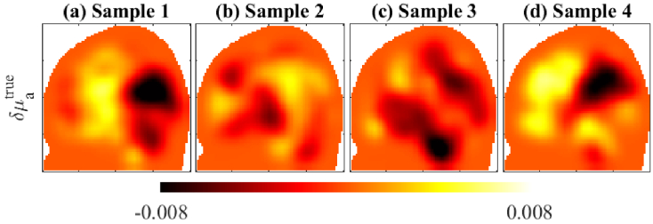
To train the neural-networks, we drew ${\mathrm{N}}_{\mathrm{s}\mathrm{a}\mathrm{m}\mathrm{p}}=2000$ ground-truth samples of $\{{\mu }_{\mathrm{a},1}^{\mathrm{t}\mathrm{r}\mathrm{u}\mathrm{e}},{\mu }_{\mathrm{s},1}^{\prime \mathrm{t}\mathrm{r}\mathrm{u}\mathrm{e}},\delta {\mu }_{\mathrm{a}}^{\mathrm{t}\mathrm{r}\mathrm{u}\mathrm{e}}{\}}^i$ . In these samples, the baseline optical parameters for the different brain compartments $\{{\mu }_{\mathrm{a},1}^{\mathrm{t}\mathrm{r}\mathrm{u}\mathrm{e}},{\mu }_{\mathrm{s},1}^{\prime \mathrm{t}\mathrm{r}\mathrm{u}\mathrm{e}}\}$ were specified by drawing random values from a uniform random distribution. The uniform distribution has its lower limit as the values specified in Table 1, and its upper limit as 40% higher than those. Meaning that the network training was intended to correct up to 40% variations to the values specified in Table 1. The absorption perturbations $\{\delta {\mu }_{\mathrm{a}}^{\mathrm{t}\mathrm{r}\mathrm{u}\mathrm{e}}\}$ were specified as smoothly varying distributions, by drawing samples from a Gaussian (Orstein-Uhlenbeck) prior distribution [30]. To prevent the CNNs from over-fitting the training images to noise, those training samples were smoothed by a 3-D Gaussian smoothing kernel, using MATLAB function ‘imgaussfilt3’. This process reduces noise and emphasizes important features of the image [61]. In this case, the spread and distribution of the absorption changes were emphasized over the noisy pixel-to-pixel variations. A few example samples are shown in Fig. 4. The training time for one subject model is displayed in Table 2. The training times were similar across all the subjects because the meshes were of similar sizes and their training used the same number of image samples, basis, and epochs.

Fig. 4.

Four samples of absorption perturbations ( $\delta {\mu }_{\mathrm{a}}^{\mathrm{t}\mathrm{r}\mathrm{u}\mathrm{e}}$ ) used in training. Parameters units are in ${\mathrm{mm}}^{-1}$ .

Table 2. Training time of the learned post-processing step for one subject and evaluation times for the reference, conventional and post-processed estimate for one sample, in hours (h) or seconds (s).

Subject	Training time	Evaluation time for one sample
	( ${\mathrm{N}}_{\mathrm{s}\mathrm{a}\mathrm{m}\mathrm{p}}=2000$ )	Reference	Conventional	Post-processed
1	98h	163s	162s	165s

3.4. Estimation

For computing MAP estimates (10), the simulated measurement data corrupted with noise (19) was used. The noise covariances were assumed known. The estimates were computed in the same mesh that was used to generate the data, to avoid model errors due to discretisation. To compare the estimated absorption changes with the (true) target absorption change, we computed three kinds of estimates:

Reference estimate: The reference estimate used the target baseline optical parameters ( ${\mu }_{\mathrm{a},1}^{\mathrm{t}\mathrm{r}\mathrm{u}\mathrm{e}},{\mu }_{\mathrm{s},1}^{\prime \mathrm{t}\mathrm{r}\mathrm{u}\mathrm{e}}$ ), to compute the Jacobian and MAP estimate, Eq. (10). These estimates present the most accurate estimates, without errors due to inaccurate baseline optical parameters.

Conventional estimate: The conventional estimates used the optical parameters mentioned in Table 1 to compute the Jacobian and MAP estimate, Eq. (10). This led to modeling errors when the measurement data was generated with target baseline parameters ( ${\mu }_{\mathrm{a},1}^{\mathrm{t}\mathrm{r}\mathrm{u}\mathrm{e}},{\mu }_{\mathrm{s},1}^{\prime \mathrm{t}\mathrm{r}\mathrm{u}\mathrm{e}}$ ) different from the values mentioned in Table 1.

Post-processed estimate: The post-processed estimates $\delta {\mu }_{\mathrm{a}}^{\mathrm{p}\mathrm{o}\mathrm{s}\mathrm{t}}$ were obtained by applying the trained CNNs on the conventional estimate, Eq. (11). The trained CNNs compensate the model errors in the conventional estimates.

3.4.1. Evaluation metrics

To evaluate the accuracy of the three estimates in terms of contrast and localisation, we used the following three metrics, utilised in earlier brain imaging studies [11]:

Contrast error: The error in the contrast of an estimated image $\delta {\hat{\mu }}_{\mathrm{a}}$ was quantified using the relative percentage error

$$\mathrm{E}(\delta {\mu }_{\text{a}})=\frac{\Vert \delta {\hat{\mu }}_{\mathrm{a}}-\delta {\mu }_{\mathrm{a}}^{\mathrm{t}\mathrm{r}\mathrm{u}\mathrm{e}}\Vert }{\Vert \delta {\mu }_{\mathrm{a}}^{\mathrm{t}\mathrm{r}\mathrm{u}\mathrm{e}}\Vert }\times 100\mathrm{\%},$$ (20)

where $\delta {\mu }_{\mathrm{a}}^{\mathrm{t}\mathrm{r}\mathrm{u}\mathrm{e}}$ is the (true) target image of the absorption parameter change.

Position error: The position error was quantified by computing the Euclidean distance between the center of mass of the estimated image from the center of mass of the target image.

Area error: The area error was quantified by computing the dice coefficient between the estimated image and the target image. The dice coefficient was the ratio of the overlapping voxels between estimated and target activation to the total number of activated voxels [11]. The activation voxels in an image were specified as the areas displaying values higher than 1% of the peak (maximum) values.

4. Results

4.1. Effects on estimated images

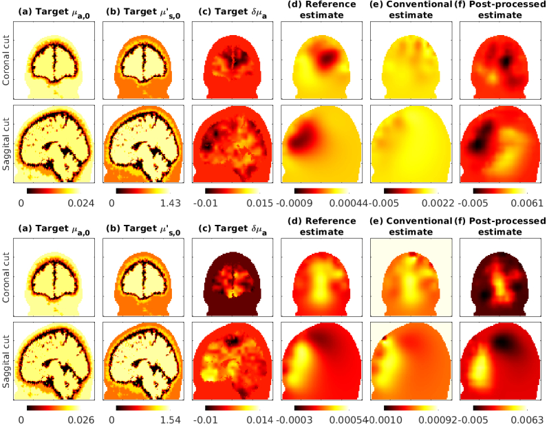
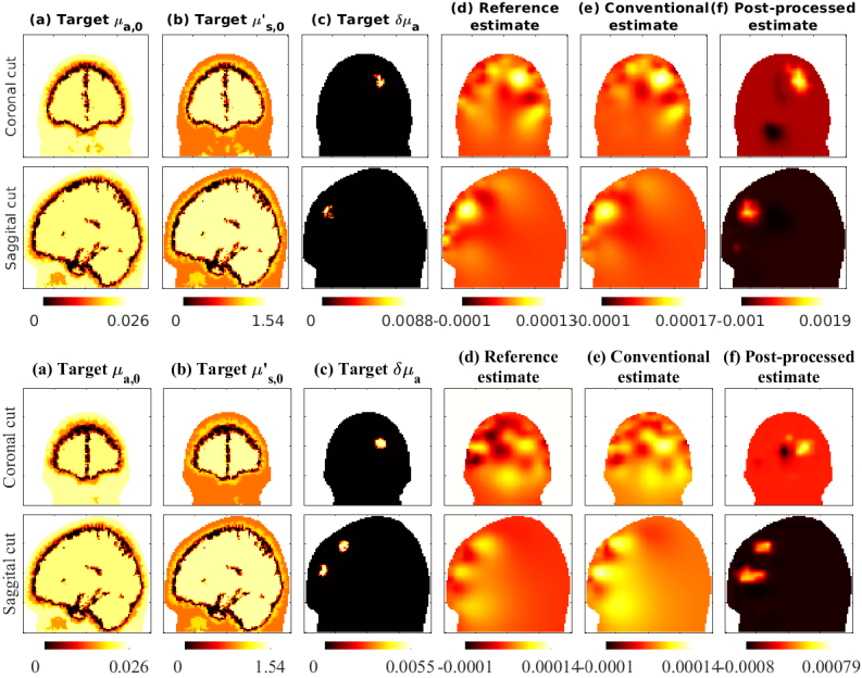
In Fig. 5 we show the estimates obtained with the subject 1 atlas. As seen in the reference estimates, the changes in absorption in the forehead region, which are closer to the sources and detectors are estimated more accurately. This was expected as the sources and detectors were placed near the forehead (Fig. 3). We also show conventional estimates obtained with 30% and 40% errors in the assumed baseline optical parameters, that show distortion and reduced contrast. The post-processed images using CNNs trained with 40% errors show improved contrast and spatial distribution.

Fig. 5.

Subject 1 evaluation with 30% errors (top two rows) and 40% errors (bottom two rows). The post-processing network was trained with up to 40% errors. Coronal (top) and Saggital (bottom) views of parameters are shown. The columns show: (a) baseline target absorption coefficient, (b) scattering coefficient, and (c) change in absorption coefficient, followed by (d) reference estimate, (e) conventional estimate in presence of errors and (f) post-processed images.

In Fig. 6 we show estimates obtained with targets that had distinct (spherical) activation regions below the forehead. Figure 6(top two rows) shows a target with an activation area specified in grey matter. Figure 6(bottom two rows) shows a target with two spherical activation areas, that contained both grey and white matter. The conventional images show distortion of the activation spot shape and location, due to the errors in assumed baseline optical parameters. The post-processed images show improved shape and localisation of the activation spot. Note that these evaluations are ‘out-of-distribution’ cases, as the training of the CNNs were performed with absorption image samples with Gaussian spatial distribution (Fig. 4), while the evaluation cases had distinct regions of activation. This show that the training the CNNs using the Gaussian spatial distribution, can also apply to other possible absorption distributions.

Fig. 6.

Evaluation with ‘out-of-distribution’ targets showing distinct activation regions. Top two rows demonstrates a case with one activation region, and bottom two rows demonstrates a case with two activation regions. Subject 1 was used in this evaluation case. Conventional and post-processed cases had 40% errors in optical parameters. The post-processing network was trained with up to 40% errors.

4.2. Statistics of estimation errors

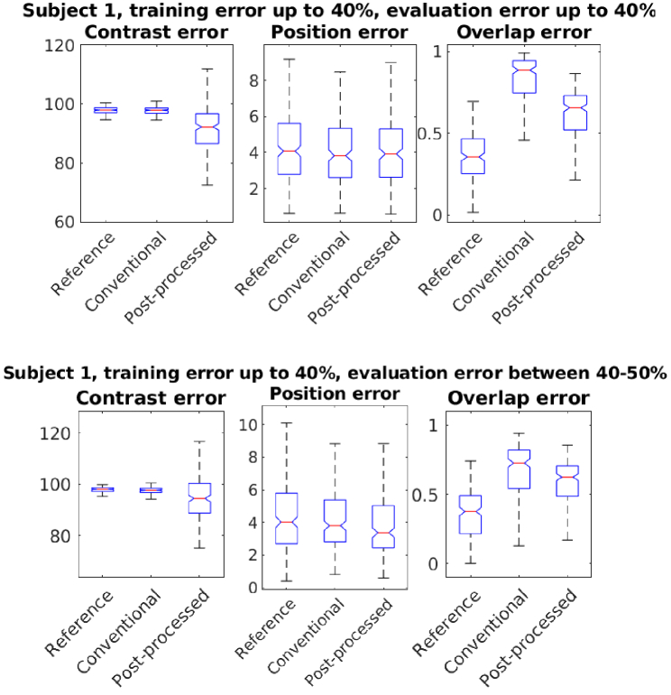
In Fig. 7 we show the statistics of errors from 400 evaluation cases, that had varying target baseline optical parameters and absorption change distributions. The training and evaluation was carried out on the Subject 1 atlas. As shown, we obtain improvement in the contrast and overlap area of the estimated images, using the proposed post-processing technique. The method show improvements when the evaluation was carried out with same level of errors (40% variation) or higher errors (40%-50% variation) in baseline parameters. This show that the method has some tolerance to errors higher than errors used in its training.

Fig. 7.

Statistics of errors in contrast, position and overlap of activation regions using reference, conventional and post-processed methods. The post-processing network was trained with up to 40% errors. Conventional and post-processed cases had up to 40% errors (top row), 40%-50% errors (bottom row) in optical parameters.

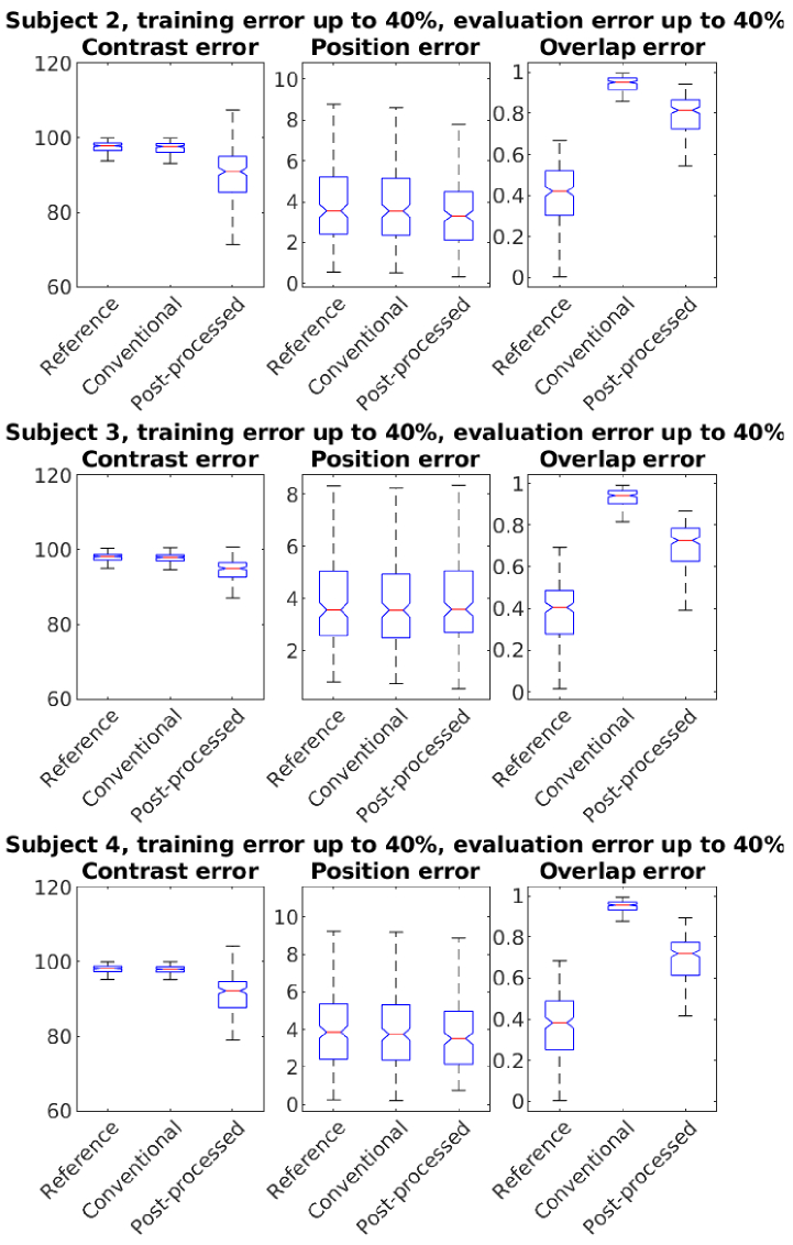
In Fig. 8 we show the statistics of errors using the atlases of Subjects 2-4. As seen in Figs. 7, 8, the proposed post-processing technique reduces the errors in the conventional estimates. The error values and their improvements vary across the different subjects, possibly due to their structural differences.

Fig. 8.

Statistics of errors in subjects 2-4 (top to bottom). The post-processing network was trained with up to 40% errors. Conventional and post-processed cases had up to 40% errors in baseline optical parameters.

We observed clear improvements in overlapping voxels (Dice coefficient). Improvements in the center of mass position were negligible for Subjects 1 and 3. Post-processing improved image contrast, but errors remained wide. Training data variability, drawn from a Gaussian prior, likely caused varying contrast in CNN outputs. This variability, however, helps the model adapt to out-of-distribution targets, which is beneficial.

5. Discussion

We studied the effects of erroneously specified baseline optical parameters in DOT brain imaging with simulations on four adult brain atlases shown in Fig. 2. The images of the estimates shown in Figs. 5, 6 and the statistics of errors shown in Figs. 7, 8 show that errors in optical base line parameters can cause large errors in the estimates.

We also developed and tested a post-processing technique to compensate for the modeling errors caused by choosing approximate baseline optical parameters. The proposed technique improved the DOT estimates, as shown in Figs. 5–8. The presented method does not require significant computational resources to carry out the post-processing, as shown in Table 2. However, the (off-line) training of the neural networks required around four days.

In this work, we have not considered other errors or uncertainties related to DOT brain imaging, such as motion artifacts, mixing of signals due to scalp blood flow, the unknown shape of the brain, or the approximately known locations of sources and detectors. Modeling and marginalization of such errors has been considered using the ‘Bayesian approximation error (BAE) method’ earlier in Refs. [21,62,63]. In our tests, the BAE method proved unsuccessful in marginalization of errors due to baseline optical parameters. The BAE method assumes errors to be normally distributed, which can be restrictive in certain cases to describe complicated errors [64] .

We have considered the segmentation of the head into four tissue types with constant optical properties. This is a strong simplification of the very complex heterogeneous anatomy of the brain, where the optical properties change constantly, for example, due to the pulsation of blood.

When trained on limited datasets, CNNs may not learn the full complexity of the data distribution. Hence, increasing the diversity of training data to improve generalization, for example, using generalized Gaussian field distributions, can help the method adapt to out-of-distribution cases.

Here, we carried out simulations in adult head models where the light propagation is severely attenuated. We note that the severity of the errors might be lower in infants’ or children’s brains. The CNNs used in this work and their training procedure could be further optimised, for example using more GPUs in parallel, which can possibly improve the training times and results. However, these choices also depend on other factors such as the measurement geometry, the chosen optical parameters, noise, etc. In the future, we will consider these factors as we extend the proposed methods to real data.

6. Conclusions

Our results show that errors in baseline optical parameters can cause large errors in DOT brain imaging. Post-processing of the estimates using pre-trained CNNs can reduce these errors, improving contrast and localisation of brain activation. We have reported the statistics of errors in estimated images, and improvements using the trained CNNs, from four subject atlases. The practical implication of this work is the improvement in robustness and accuracy of DOT brain imaging. In the future, the proposed post-processing technique can be trained using data from other subjects and applied to enhance brain imaging with real-world data.

Funding

Research Council of Finland10.13039/501100002341 (320166, 338408, 353086, 353093, 358944, 359186); European Union’s Horizon 2020 research and innovation program (101001417); EU's research and innovation funding programme (INFRAIA-2016-1-730897); Ministerio de Economía y Competitividad10.13039/501100003329 (PID2020-115088RB-I00); Finnish Cultural Foundation10.13039/501100003125 (00200746).

Disclosures

The authors declare no conflicts of interest.

Data availability

Data underlying the results presented in this paper are not publicly available at this time but may be obtained from the authors upon reasonable request.

References

- 1.Arridge S. R., “Optical tomography in medical imaging,” Inverse Problems 15(2), R41–R93 (1999). 10.1088/0266-5611/15/2/022 [DOI] [Google Scholar]
- 2.Gibson A., Hebden J., Arridge S. R., “Recent advances in diffuse optical imaging,” Phys. Med. Biol. 50(4), R1–R43 (2005). 10.1088/0031-9155/50/4/R01 [DOI] [PubMed] [Google Scholar]
- 3.Durduran T., Choe R., Baker W. B., et al. , “Diffuse optics for tissue monitoring and tomography,” Rep. Prog. Phys. 73(7), 076701 (2015). 10.1088/0034-4885/73/7/076701 [DOI] [PMC free article] [PubMed] [Google Scholar]
- 4.Hoshi Y., Yamada Y., “Overview of diffuse optical tomography and its clinical applications,” J. Biomed. Opt. 21(9), 091312 (2016). 10.1117/1.JBO.21.9.091312 [DOI] [PubMed] [Google Scholar]
- 5.Hernandez-Martin E., Gonzalez-Mora J. L., “Diffuse optical tomography in the human brain: a briefly review from the neurophysiology to its applications,” Brain Science Advances 6(4), 289–305 (2020). 10.26599/BSA.2020.9050014 [DOI] [Google Scholar]
- 6.Wheelock M. D., Culver J. P., Eggebrecht A. T., “High-density diffuse optical tomography for imaging human brain function,” Rev. Sci. Instrum. 90(5), 051101 (2019). 10.1063/1.5086809 [DOI] [PMC free article] [PubMed] [Google Scholar]
- 7.Okada E., Delpy D. T., “Near-infrared light propagation in an adult head model. I. Modeling of low-level scattering in the cerebrospinal fluid layer,” Appl. Opt. 42(16), 2906–2914 (2003). 10.1364/AO.42.002906 [DOI] [PubMed] [Google Scholar]
- 8.Schweiger M., Arridge S., “Optical tomographic reconstruction in a complex head model using a priori region boundary information,” Phys. Med. Biol. 44(11), 2703–2721 (1999). 10.1088/0031-9155/44/11/302 [DOI] [PubMed] [Google Scholar]
- 9.Zhan Y., Eggebrecht A. T., Culver J. P., et al. , “Image quality analysis of high-density diffuse optical tomography incorporating a subject-specific head model,” Front. Neuroenerg. 4, 6 (2012). 10.3389/fnene.2012.00006 [DOI] [PMC free article] [PubMed] [Google Scholar]
- 10.Custo A., Boas D. A., Tsuzuki D., et al. , “Anatomical atlas-guided diffuse optical tomography of brain activation,” NeuroImage 49(1), 561–567 (2010). 10.1016/j.neuroimage.2009.07.033 [DOI] [PMC free article] [PubMed] [Google Scholar]
- 11.Ferradal S. L., Eggebrecht A. T., Hassanpour M., et al. , “Atlas-based head modeling and spatial normalization for high-density diffuse optical tomography: in vivo validation against fmri,” NeuroImage 85, 117–126 (2014). 10.1016/j.neuroimage.2013.03.069 [DOI] [PMC free article] [PubMed] [Google Scholar]
- 12.Boas D. A., Culver J. P., Stott J. J., et al. , “Three dimensional Monte Carlo code for photon migration through complex heterogeneous media including the adult human head,” Opt. Express 10(3), 159–170 (2002). 10.1364/OE.10.000159 [DOI] [PubMed] [Google Scholar]
- 13.Firbank M., Arridge S. R., Schweiger M., et al. , “An investigation of light transport through scattering bodies with non-scattering regions,” Phys. Med. Biol. 41(4), 767–783 (1996). 10.1088/0031-9155/41/4/012 [DOI] [PubMed] [Google Scholar]
- 14.Ripoll J., Nieto-Vesperinas M., Arridge S. R., et al. , “Boundary conditions for light propagation in diffusive media with nonscattering regions,” J. Opt. Soc. Am. A 17(9), 1671–1681 (2000). 10.1364/JOSAA.17.001671 [DOI] [PubMed] [Google Scholar]
- 15.Tarvainen T., Vauhkonen M., Kolehmainen V., et al. , “Coupled radiative transfer equation and diffusion approximation model for photon migration in turbid medium with low-scattering and non-scattering regions,” Phys. Med. Biol. 50(20), 4913–4930 (2005). 10.1088/0031-9155/50/20/011 [DOI] [PubMed] [Google Scholar]
- 16.Ripoll J., Nieto-Vesperinas M., Arridge S. R., “Effect of roughness in nondiffusive regions within diffusive media,” J. Opt. Soc. Am. A 18(4), 940–947 (2001). 10.1364/JOSAA.18.000940 [DOI] [Google Scholar]
- 17.Custo A., Wells Iii W. M., Barnett A. H., et al. , “Effective scattering coefficient of the cerebral spinal fluid in adult head models for diffuse optical imaging,” Appl. Opt. 45(19), 4747–4755 (2006). 10.1364/AO.45.004747 [DOI] [PubMed] [Google Scholar]
- 18.Prince S., Kolehmainen V., Kaipio J. P., et al. , “Time-series estimation of biological factors in optical diffusion tomography,” Phys. Med. Biol. 48(11), 1491–1504 (2003). 10.1088/0031-9155/48/11/301 [DOI] [PubMed] [Google Scholar]
- 19.Gregg N. M., White B. R., Zeff B. W., et al. , “Brain specificity of diffuse optical imaging: improvements from superficial signal regression and tomography,” Front. Neuroenerg. 2, 14 (2010). 10.3389/fnene.2010.00014 [DOI] [PMC free article] [PubMed] [Google Scholar]
- 20.Culver J. P., Siegel A. M., Stott J. J., et al. , “Volumetric diffuse optical tomography of brain activity,” Opt. Lett. 28(21), 2061–2063 (2003). 10.1364/OL.28.002061 [DOI] [PubMed] [Google Scholar]
- 21.Mozumder M., Tarvainen T., Kaipio J. P., et al. , “Compensation of modeling errors due to unknown domain boundary in diffuse optical tomography,” J. Opt. Soc. Am. A 31(8), 1847–1855 (2014). 10.1364/JOSAA.31.001847 [DOI] [PubMed] [Google Scholar]
- 22.Jin K. H., McCann M. T., Froustey E., et al. , “Deep convolutional neural network for inverse problems in imaging,” IEEE Trans. Imag. Process. 26(9), 4509–4522 (2017). 10.1109/TIP.2017.2713099 [DOI] [PubMed] [Google Scholar]
- 23.Kang E., Min J., Ye J. C., “A deep convolutional neural network using directional wavelets for low-dose X-ray CT reconstruction,” Med. Phys. 44(10), e360–e375 (2017). 10.1002/mp.12344 [DOI] [PubMed] [Google Scholar]
- 24.Adler J., Öktem O., “Solving ill-posed inverse problems using iterative deep neural networks,” Inverse Problems 33(12), 124007 (2017). 10.1088/1361-6420/aa9581 [DOI] [Google Scholar]
- 25.Feng J., Sun Q., Li Z., et al. , “Back-propagation neural network-based reconstruction algorithm for diffuse optical tomography,” J. Biomed. Opt. 24(05), 1 (2018). 10.1117/1.JBO.24.5.051407 [DOI] [PMC free article] [PubMed] [Google Scholar]
- 26.Fan Y., Ying L., “Solving optical tomography with deep learning,” arXiv, (2019). 10.48550/arXiv.1910.04756 [DOI]
- 27.Sabir S., Cho S., Kim Y., et al. , “Convolutional neural network-based approach to estimate bulk optical properties in diffuse optical tomography,” Appl. Opt. 59(5), 1461–1470 (2020). 10.1364/AO.377810 [DOI] [PubMed] [Google Scholar]
- 28.Yoo J., Sabir S., Heo D., et al. , “Deep learning diffuse optical tomography,” IEEE Trans. Med. Imag. 39(4), 877–887 (2019). 10.1109/TMI.2019.2936522 [DOI] [PubMed] [Google Scholar]
- 29.Zou Y., Zeng Y., Li S., et al. , “Machine learning model with physical constraints for diffuse optical tomography,” Biomed. Opt. Express 12(9), 5720–5735 (2021). 10.1364/BOE.432786 [DOI] [PMC free article] [PubMed] [Google Scholar]
- 30.Mozumder M., Hauptmann A., Nissilä I., et al. , “A model-based iterative learning approach for diffuse optical tomography,” IEEE Trans. Med. Imaging 41(5), 1289–1299 (2021). 10.1109/TMI.2021.3136461 [DOI] [PubMed] [Google Scholar]
- 31.Maier A. K., Syben C., Stimpel B., et al. , “Learning with known operators reduces maximum error bounds,” Nature machine intelligence 1(8), 373–380 (2019). 10.1038/s42256-019-0077-5 [DOI] [PMC free article] [PubMed] [Google Scholar]
- 32.Aggarwal H. K., Mani M. P., Jacob M., “MoDL: model-based deep learning architecture for inverse problems,” IEEE Trans. Med. Imaging 38(2), 394–405 (2018). 10.1109/TMI.2018.2865356 [DOI] [PMC free article] [PubMed] [Google Scholar]
- 33.Hauptmann A., Lucka F., Betcke M., et al. , “Model-based learning for accelerated, limited-view 3-D photoacoustic tomography,” IEEE Trans. Med. Imag. 37(6), 1382–1393 (2018). 10.1109/TMI.2018.2820382 [DOI] [PMC free article] [PubMed] [Google Scholar]
- 34.Choi J. H., Wolf M., Toronov V. Y., et al. , “Noninvasive determination of the optical properties of adult brain: near-infrared spectroscopy approach,” J. Biomed. Opt. 9(1), 221–229 (2004). 10.1117/1.1628242 [DOI] [PubMed] [Google Scholar]
- 35.Farina A., Torricelli A., Bargigia I., et al. , “In-vivo multilaboratory investigation of the optical properties of the human head,” Biomed. Opt. Express 6(7), 2609–2623 (2015). 10.1364/BOE.6.002609 [DOI] [PMC free article] [PubMed] [Google Scholar]
- 36.Bevilacqua F., Piguet D., Marquet P., et al. , “In vivo local determination of tissue optical properties: applications to human brain,” Appl. Opt. 38(22), 4939–4950 (1999). 10.1364/AO.38.004939 [DOI] [PubMed] [Google Scholar]
- 37.Franceschini M. A., Fantini S., Thompson J. H., et al. , “Hemodynamic evoked response of the sensorimotor cortex measured noninvasively with near-infrared optical imaging,” Psychophysiology 40(4), 548–560 (2003). 10.1111/1469-8986.00057 [DOI] [PMC free article] [PubMed] [Google Scholar]
- 38.Bartlett M. F., Jordan S. M., Hueber D. M., et al. , “Impact of changes in tissue optical properties on near-infrared diffuse correlation spectroscopy measures of skeletal muscle blood flow,” J. Appl. Physiol. 130(4), 1183–1195 (2021). 10.1152/japplphysiol.00857.2020 [DOI] [PMC free article] [PubMed] [Google Scholar]
- 39.Heiskala J., Hiltunen P., Nissilä I., “Significance of background optical properties, time-resolved information and optode arrangement in diffuse optical imaging of term neonates,” Phys. Med. Biol. 54(3), 535–554 (2009). 10.1088/0031-9155/54/3/005 [DOI] [PubMed] [Google Scholar]
- 40.Ishimaru A., Wave Propagation and Scattering in Random Media (Academic, 1978). [Google Scholar]
- 41.Schweiger M., Arridge S. R., Hiraoka M., et al. , “The finite element method for the propagation of light in scattering media: boundary and source conditions,” Med. Phys. 22(11), 1779–1792 (1995). 10.1118/1.597634 [DOI] [PubMed] [Google Scholar]
- 42.Arridge S., Schweiger M., Hiraoka M., et al. , “A finite element approach for modeling photon transport in tissue,” Med. Phys. 20(2), 299–309 (1993). 10.1118/1.597069 [DOI] [PubMed] [Google Scholar]
- 43.Mozumder M., Tarvainen T., Seppänen A., et al. , “Nonlinear approach to difference imaging in diffuse optical tomography,” J. Biomed. Opt. 20(10), 105001 (2015). 10.1117/1.JBO.20.10.105001 [DOI] [PubMed] [Google Scholar]
- 44.Kingma D. P., Ba J., “Adam: a method for stochastic optimization,” arXiv, (2014). 10.48550/arXiv.1412.69800 [DOI]
- 45.Herzberg W., Rowe D. B., Hauptmann A., et al. , “Graph convolutional networks for model-based learning in nonlinear inverse problems,” IEEE Trans. Comput. Imaging 7, 1341–1353 (2021). 10.1109/TCI.2021.3132190 [DOI] [PMC free article] [PubMed] [Google Scholar]
- 46.Herzberg W., Hauptmann A., Hamilton S. J., “Domain independent post-processing with graph u-nets: applications to electrical impedance tomographic imaging,” Physiol. Meas. 44(12), 125008 (2023). 10.1088/1361-6579/ad0b3d [DOI] [PMC free article] [PubMed] [Google Scholar]
- 47.Schweiger M., Arridge S. R., “The Toast++ software suite for forward and inverse modeling in optical tomography,” J. Biomed. Opt. 19(4), 040801 (2014). 10.1117/1.JBO.19.4.040801 [DOI] [PubMed] [Google Scholar]
- 48.Abadi M., Barham P., Chen J., et al. , “Tensorflow: a system for large-scale machine learning,” in 12th USENIX Symposium on Operating Systems Design and Implementation (OSDI 16) (2016), pp. 265–283. [Google Scholar]
- 49.Tran A. P., Yan S., Fang Q., “Improving model-based functional near-infrared spectroscopy analysis using mesh-based anatomical and light-transport models,” Neurophotonics 7(01), 1 (2020). 10.1117/1.NPh.7.1.015008 [DOI] [PMC free article] [PubMed] [Google Scholar]
- 50.Aubert-Broche B., Griffin M., Pike G. B., et al. , “Twenty new digital brain phantoms for creation of validation image data bases,” IEEE Trans. Med. Imag. 25(11), 1410–1416 (2006). 10.1109/TMI.2006.883453 [DOI] [PubMed] [Google Scholar]
- 51.Strangman G., Franceschini M. A., Boas D. A., “Factors affecting the accuracy of near-infrared spectroscopy concentration calculations for focal changes in oxygenation parameters,” NeuroImage 18(4), 865–879 (2003). 10.1016/S1053-8119(03)00021-1 [DOI] [PubMed] [Google Scholar]
- 52.Franceschini M. A., Boas D. A., “Noninvasive measurement of neuronal activity with near-infrared optical imaging,” NeuroImage 21(1), 372–386 (2004). 10.1016/j.neuroimage.2003.09.040 [DOI] [PMC free article] [PubMed] [Google Scholar]
- 53.https://www.rp-photonics.com/noise_equivalent_power.html. [Online; accessed 22.5.2024].
- 54.https://www.thorlabs.com/images/TabImages/Noise_Equivalent_Power_White_Paper.pdf. [Online; accessed 22.5.2024].
- 55.https://www.osioptoelectronics.com/media/pages/knowledgebase/b954012b64-1675100541/an-photodiode-parameters-and-characteristics.pdf. [Online; accessed 22.5.2024].
- 56.Nissilä I. T., “Instrumentation for medical optical tomography with applications,” Ph.D. thesis, Helsinki University of Technology, Department of Engineering Physics and Mathematics (2004).
- 57.Rogalski A., Bielecki Z., “Detection of optical radiation,” Bull. Pol. Acad. Sci.: Tech. Sci. 52(1), 1 (2004). 10.4064/ba52-1-1 [DOI] [Google Scholar]
- 58.Korneev A., Matvienko V., Minaeva O., et al. , “Quantum efficiency and noise equivalent power of nanostructured, nbn, single-photon detectors in the wavelength range from visible to infrared,” IEEE Trans. Appl. Supercond. 15(2), 571–574 (2005). 10.1109/TASC.2005.849923 [DOI] [Google Scholar]
- 59.Richards P., “Bolometers for infrared and millimeter waves,” J. Appl. Phys. 76(1), 1–24 (1994). 10.1063/1.357128 [DOI] [Google Scholar]
- 60.Eggebrecht A. T., Ferradal S. L., Robichaux-Viehoever A., et al. , “Mapping distributed brain function and networks with diffuse optical tomography,” Nat. Photonics 8(6), 448–454 (2014). 10.1038/nphoton.2014.107 [DOI] [PMC free article] [PubMed] [Google Scholar]
- 61.Kusrini K., Yudianto M. R. A., Al Fatta H., “The effect of Gaussian filter and data preprocessing on the classification of Punakawan puppet images with the convolutional neural network algorithm,” International Journal of Electrical and Computer Engineering 12, 3752 (2022). 10.11591/ijece.v12i4.pp3752-3761 [DOI] [Google Scholar]
- 62.Heiskala J., Kolehmainen V., Tarvainen T., et al. , “Approximation error method can reduce artifacts due to scalp blood flow in optical brain activation imaging,” J. Biomed. Opt. 17(9), 0960121 (2012). 10.1117/1.JBO.17.9.096012 [DOI] [PubMed] [Google Scholar]
- 63.Mozumder M., Tarvainen T., Arridge S. R., et al. , “Compensation of optode sensitivity and position errors in diffuse optical tomography using the approximation error approach,” Biomed. Opt. Express 4(10), 2015–2031 (2013). 10.1364/BOE.4.002015 [DOI] [PMC free article] [PubMed] [Google Scholar]
- 64.Lunz S., Hauptmann A., Tarvainen T., et al. , “On learned operator correction in inverse problems,” SIAM J. Imaging Sci. 14(1), 92–127 (2021). 10.1137/20M1338460 [DOI] [Google Scholar]
Associated Data
This section collects any data citations, data availability statements, or supplementary materials included in this article.
Data Availability Statement