Neural network-based reconstruction of steady-state temperature systems with unknown material composition

Abstract

Effective thermal management is crucial for the performance and longevity of devices such as computer chips and batteries. A fundamental challenge in this field is accurately determining temperature distributions, which are often limited by incomplete observations. We introduce a neural-network-based approach to overcome these challenges. Specifically, a physics-informed fully convolutional auto-encoder coupled with a preceding spatial propagator network module is used to reconstruct complete temperature fields from partial observations, without requiring additional information about the spatial distribution of materials with varying thermal properties. This paper details the development and validation of our model, demonstrating its effectiveness in virtual sensing setups for both simulated and real-world thermal systems. The reconstruction capabilities for different sampling strategies are investigated. The most challenging of which is the “grid-edge” sampling where only discrete temperature sensors on the periphery of the systems are taken as input, amounting to a sampling ratio as low as 3.12%. The presented method is able to reconstruct the full temperature field with a relative average error of 1.1%. The NN-based approach outperforms the standard Kriging method in predicting the maximum temperature in a system, and proves more robust when the available measurements contain little information.

Introduction

In the realm of electronic device optimization, understanding and controlling thermal properties is crucial. Devices like power electronic chips or batteries are particularly sensitive to temperature variations, as these can lead to energy inefficiencies, heat leakages, and accelerated material degradation. Traditionally, obtaining a comprehensive picture of temperature fields within these devices has been a challenge. Measurement techniques are often limited by practical constraints, leading to partial or incomplete temperature data. This lack of complete thermal information hinders the ability to optimize devices for better performance and longevity.

Computational methods in the area of virtual sensing address these challenges by inferring or estimating quantities of interest from the available information. Virtual sensing has been traditionally based on a combination of classical regression and statistical techniques^1–4. Motivated by the success of machine learning (ML) in many scientific and engineering domains, there has been a surge of works applying a variety of ML techniques to approximate physical fields. For instance, ML has been successfully applied as fast alternative to physics-based simulations for specific sets of geometries, material properties and boundary conditions^5–8. While these contributions aim for the direct approximation of the physical field based on known input parameters, virtual sensing focuses on an incompletely defined problems where the inputs are only partially known, for instance, the exact boundary conditions or distribution of materials might be unknown, but additionally some measurement points of the physical field of interest are available. This lack of information makes the application of standard physics-based methods, e.g. the finite element method, infeasible or requires numerous optimization iterations. However, it has been demonstrated in numerous cases that ML methods can efficiently solve inverse problems, where for instance the conductivity distribution in simple geometries is approximated based on the known full temperature field⁹, or, properties of fluid mechanics can be estimated based on scarce data¹⁰.

These successes make it plausible that ML can play a major role in virtual sensing, as has been demonstrated recently. In¹¹ the authors present a physics informed generative adversarial network (GAN) to predict missing field values of a magnetic field in 2D. In¹² a convolutional neural network is used to predict the steady-state temperature field of a system, given a known heat source layout and boundary conditions, without labelled data, purely from the physics-inspired loss function. In¹³, a physics-informed neural network (PINN^14,15) was employed as a fast surrogate model for heat conduction problems in 1D, 2D and 3D. Very similar to our work is¹⁶. In this study, also a PINN was proposed as a virtual thermal sensor that uses data measured by a small number of sensors to estimate the full temperature field in a silicon 2D system, assuming the boundary conditions and the positions and values of heat sources are known.

In this work, we present a model that uses a fully convolutional autoencoder to predict the full temperature field of a 2D system with heterogenous material properties, based on a number of sampling points. We assume blind virtual sensing, with no knowledge of the materials that form the system, or the boundary conditions, or the number, positions and values of the heat sources inside the system. In this way, our model prepares the ground for a virtual sensor in a realistic scenario where most such information is unknown or difficult to estimate. Working in 2D, we perform a proof-of-principle study of the feasibility of blind virtual sensors. Moreover, we provide an experimental validation of our models in a simplified real system.

The paper is organized as follows. In Section “Data generation” we describe the training and validation datasets generation process, based on finite element simulations. The neural network architecture and training methodologies are discussed in Section “Method for temperature reconstruction”. The results for the simulated data are presented in Section “Results”. In Section “Extreme examples” we show some extreme applications of our models, as well as the results for measurements in a real system (Section “Experimental evaluation”). We compare our ML model with the more classical Kriging method in Section “Comparison with Kriging”. The overall approach of this research is illustrated in Fig. 1.

Fig. 1.

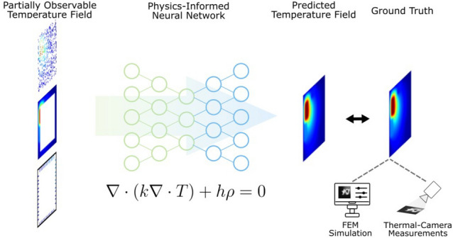
Illustration of the neural network setup for predicting temperature distributions in a 2D system.

Data generation

An envisioned future application of our virtual sensing model is the monitoring of a system of surface-mounted components, which we assume here can be approximated by a 2D system. The training is performed using supervised learning with steady-state finite element (FEM) simulations of those systems as ground truth.

Drawing from previous experience^17,18, the training of neural networks in this application domain leads to better generalization if the training dataset consists of abstract geometric structures instead of realistic components¹⁹. Additionally, these abstract geometries are much simpler to generate automatically than realistic systems, as we describe below. Moreover, the performance of the networks also improves if it is exposed to very diverse material properties during training and not just to those of a reduced number of realistic materials, as well as to different operating conditions, which in the present work are modelled by the values and positions of heat sources. Similar considerations apply to the boundary and initial conditions.

The dataset we generated thus consists of 2D systems with inhomogeneous material properties (see Table 1), containing heat sources of variable magnitude and at different locations.

Table 1.

Material Properties: Different materials used in the creation of our dataset and their nominal thermal properties.

Material	Heat conductivity k (W m−1 K−1)	Specific heat capacity cp (J kg−1 K−1)	Density ρ (kg m−3)
Copper	384	385	8930
Epoxy	0.881	952	1682
Silicon	148	705	2330
FR4	0.25	1200	1900
AlO	35	880	3890
Aluminum	148	128	1930

The actual properties are chosen by randomly selecting values in the range [0.75, 1.25] around the nominal properties.

The systems were generated automatically as follows:

• A 50 mm $\times$ 50 mm square is created, acting as a canvas for the following steps. A material from Table 1 is assigned to it and its material properties are further varied by a ± 25% around their nominal values. No heat source is assigned to this element.

• Then, smaller squares (up to ten) of random sizes (between 6 and 20 mm) are placed on the canvas at random positions. If in the process two or more such squares totally or partially overlap, they are merged. To each of the resulting structures, a random material from Table 1 is assigned with their material properties randomly varied as before. Whether each of these smaller structures has a heat source or not is assigned randomly, ensuring that, at the end of the process, there is at least one heat source in the system. The values of the heat sources are randomized around a central value of ${10}^4$J/kg s.

• An initial temperature is randomly chosen for the whole system, ± 25% around 275 K.

• Neumann or Dirichlet boundary conditions are assigned randomly to each of the sides of the canvas separately. For Dirichlet, the boundary condition temperature is set to the initial temperature obtained in the point above; for Neumann, the heat transfer coefficient value is randomly set to ± 25% around a central value of 50 kg/s² K.

• For each system a conformal triangular finite-element mesh is created using the open-source meshing tool gmsh²⁰ and the steady state thermal configuration of each of these systems is calculated using the Elmer FEM simulator²¹.

• Finally, for the ML task, each system and its ground truth are turned into an image via a regular discretization with $50\times 50$ points (pixels).

Due to the random generation process, it is very difficult to ensure in advance that the final thermal configuration represents a realistic situation. For this reason, the systems produced are filtered, discarding those with maximum temperature in the system above 400K and, in addition, we keep only systems for which the difference between the maximum and minimum temperature in the system is between 20 and 100 K. In the end, we have a dataset with 775 such systems which can be augmented via 90, 180 and 270 degrees rotations to 3100 systems.

Method for temperature reconstruction

Neural network architecture

The temperature reconstruction algorithm introduced in this study can be seen as an image restoration process (see Section “Sampling”) with a deep learning approach. The network we propose is inspired by the foundational U-Net architecture²². It employs an encoding/decoding mechanism to restore the gaps in data within our virtual sensing context. A crucial aspect in our design of the neural network was to create a model that is compact in parameter size, currently consisting of 8,745,434 parameters. The goal was to ensure the model’s suitability for deployment on embedded devices. On a high-end GPU (on one out of 18 identical shards of an NVIDIA A100 80GB PCIe GPU with CUDA Version 12.4) the model achieves an inference time of approximately 3 ms. This rapid inference capability underscores the model’s potential for almost real-time applications or testing scenarios where an implementation on a less powerful device is necessary. For completeness, the time for data generation was less than one minute per system (single-core of AMD EPYC 7763 64-core processor), while the training of the NN took approx. 12 hours on one shard of the GPU. However, in a real use case time for data generation and training pays off because these tasks are performed only once while the inference can be used numerous times afterwards.

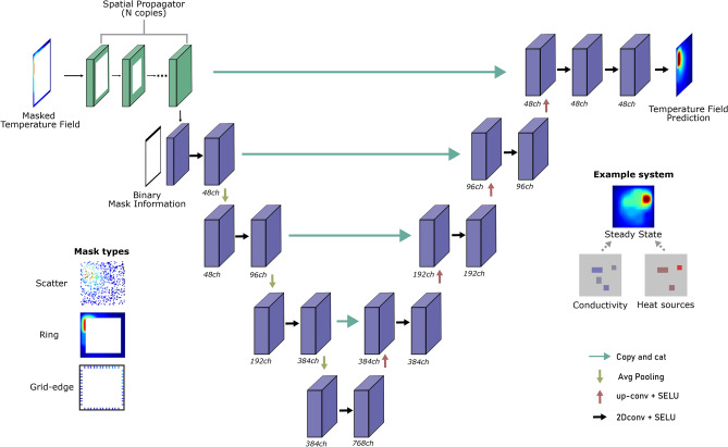
The architecture of the proposed deep learning model for temperature field reconstruction progresses from input to output as follows (see Fig. 2): The input stage accepts a masked temperature field, accommodating various masking techniques as detailed in the next section. This is followed by a spatial propagator consisting of N copies of a convolutional layer (kernel-size = 5, padding = 2, padding-mode = ’replicate’), without intermediate activation functions, designed to distribute temperature information throughout the field. This step is crucial, especially for mask types that leave the field’s center devoid of data, by gradually extending the known boundary information inward through repeated application of convolutions across the field’s periphery. The spatial propagator’s design is specifically tailored to the type of masking applied to the input field, with the number of convolutional layers adjusted according to the extent of information absence-twenty layers for square and grid-edge masking, and one layer for random masking.

Fig. 2.

Illustration of the U-Net-based neural network architecture designed for reconstructing 2D temperature fields from partially observed data. The process initiates with a ’Spatial Propagator’ that pre-processes the input masked temperature fields, followed by a U-Net for the prediction of the complete temperature distribution. The figure also presents three distinct masking approaches used in our experiments: ’Random’, ’Ring’, and ’Grid-edge’, alongside an exemplar system showcasing a randomly distributed conductivity and heat-source field, and its resulting steady-state temperature field as simulated for dataset creation.

Subsequent to the spatial propagator, binary mask information is integrated to inform the network about the locations of missing data. The encoder, comprising four layers of convolution followed by SELU activation functions and average pooling, processes the enhanced temperature field. The decoder mirrors this structure with four transposed convolutions followed by SELU activations and average pooling, incorporating residual connections from the encoder to refine the reconstruction. This process is completed by three additional convolutional layers with SELU activations, where the final output represents the predicted full temperature field.

All convolution operations in the encoder, decoder and their subsequent two layers are used with kernel-size = 3 and padding = 1. The very last layer delivering the final output for the temperature prediction uses kernel-size = 1 and default-values of the PyTorch package for the other parameters. Average pooling is used with kernel-size = 3, padding = 1 and stride = 1.

Sampling

The task of virtually sensing the temperature distribution in a system is implemented by masking certain pixels in the temperature distribution of each system (see Section “Data Generation”). The unmasked pixels thus represents sampling points or regions in a hypothetical measurement. We consider three different types of sampling of a system (see Figs. 2, 3, 4 and 5):

• Scattered sampling: In this case random temperature values over the system are sampled, with an adjustable ratio of sampling points.

• Ring sampling: A square mask is applied, which amounts to sampling values all around the border of the system. The length of the square mask can be adjusted.

• Grid-edge: In addition to the square mask above, additional masking is applied regularly along the border. This amounts to having a number of discrete measurement regions on the periphery of the system.

Fig. 3.

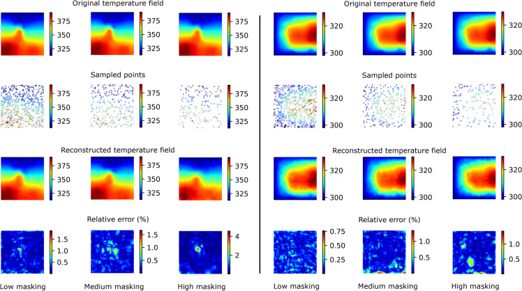
Two examples of the reconstructed temperature fields for the scattered sampling method, for three different masking ratios. The rows are, from top to bottom, the ground truth temperature, the sampled temperature values, the reconstructed temperature field and the relative error in percent (see Eq. 2). Each of the three columns per system corresponds to different masking ratios, which amounts to a different sampling ratio as described in the text.

Fig. 4.

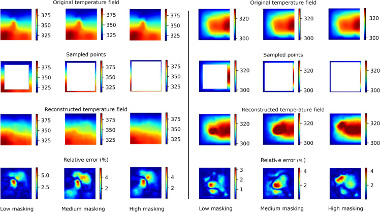
Two examples of the reconstructed temperature fields for the ring sampling method, for three different masking ratios. The rows are, from top to bottom, the ground truth temperature, the sampled temperature values, the reconstructed temperature field and the relative error in percent (see Eq. 2). Each of the three columns per system corresponds to different masking ratios, which amounts to a different sampling ratio as described in the text.

Fig. 5.

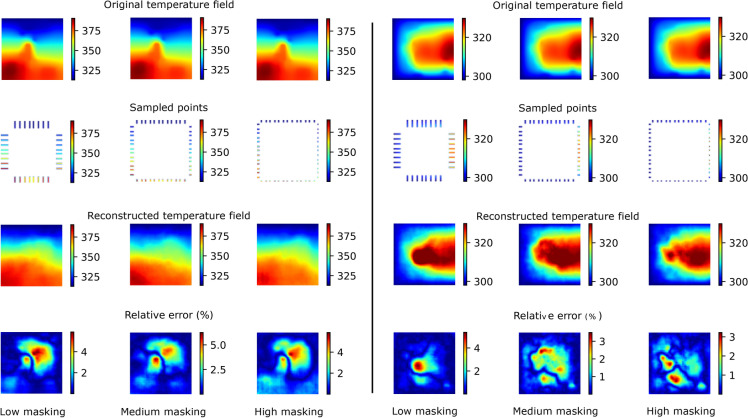
Two examples of the reconstructed temperature fields for the Grid-edge sampling method, for three different masking ratios. The rows are, from top to bottom, the ground truth temperature, the sampled temperature values, the reconstructed temperature field and the relative error in percent (see Eq. 2). Each of the three columns per system corresponds to different masking ratios, which amounts to a different sampling ratio as described in the text.

Training details

The dataset employed for training and validation follows an 80–20% split for the train-test distribution. The training process is guided by a loss function that combines Mean Squared Error (MSE) with physics-informed components to ensure not only fidelity to the observed data but also adherence to underlying physical laws. The optimization runs in all cases for 7000 epochs, with a batch size of 20, learning rate set at 0.0001, and uses the Adam optimizer for updating the model parameters. The implementation is carried out in PyTorch version 1.10.2, utilizing default parameter settings for standard neural network classes like Conv2D, if not further specified.

The loss function is designed to minimize discrepancies between the actual temperature field (T) and the reconstructed field ($T^{\prime }$), enforce gradient consistency, and comply with the constraints of the heat equation. Specifically, the training objective includes minimizing the difference in temperature fields ($L_T$), ensuring the gradient of temperature fields ($L_G$) is consistent, and satisfying the heat equation constraint ($L_H$). The total loss optimized during training is defined as:

$$\begin{array}{c}\hfill L_{\mathit{total}}={\alpha }_T·L_T+{\alpha }_G·L_G+{\alpha }_H·L_H,\end{array}$$ 1

where:

• $L_T=\frac{1}{N}{\sum }_{\mathit{pixels}}{\Vert T-T^{\prime }\Vert }^2$ measures the discrepancy in temperature fields.

• $L_G=\frac{1}{N}{\sum }_{\mathit{pixels}}{\Vert \mathrm{\nabla }T-\mathrm{\nabla }{T}^{\prime }\Vert }^2$ focuses on the gradient of temperature fields.

• $L_H=\Vert \frac{1}{N}{\sum }_{\mathit{pixels}}{C}_H(T,k,h,\rho )-\frac{1}{N}{\sum }_{\mathit{pixels}}{C}_H(T^{\prime },k,h,\rho )\Vert$ quantifies the deviation from the heat equation constraint. With, $C_H(T,k,h,\rho )=\mathrm{\nabla }·(k\mathrm{\nabla }T)+h\rho$, where k, h, and $\rho$ denote the spatially varying conductivity, heat source density and density, respectively.

With N the total number of pixels in the input image. The gradients and Laplacian in $L_G$ and $L_H$ are approximated via finite differences using custom neural network modules in PyTorch, which apply 3 $\times$ 3 filters to the temperature fields. This leads to non-negligible discretization errors in the calculation of gradients, particularly in regions where the material changes and the gradient is discontinuous. We mitigate these inaccuracies by analyzing the mean error between the ground truth and the predicted values, emphasizing the relative errors rather than absolute discrepancies. We have previously observed that a heat equation term can act as a regularization even if significant discretization errors are present in the gradient computation¹⁷. For the use as regularization term $L_H$ must be scaled to be much smaller than the $L_T$. After some exploration, the weights ${\alpha }_T,{\alpha }_G,{\alpha }_H$ were set to $[{\alpha }_T,{\alpha }_G,{\alpha }_H]=[1.0,0.1,1.0]$ in all experiments presented here. Note, that the evaluation of the finite differences is conducted in pixel-space rather than physical units to prevent disproportionately high loss-terms that would require excessively low weighting to compensate. The loss function (1) facilitates the training of a model that not only predicts temperature fields with high accuracy but is also aware of the physical principles governing heat transfer.

Results

In this section we show the results of our temperature reconstruction model using the three different sampling methods from Section “Sampling” with different ratios (Low, Medium and High) of masked values. A summary of the average reconstruction error, defined as the average relative error in percent

$$\begin{array}{c}\hfill \text{Relative Error}=\frac{1}{N}\sum _{i=1}^N\left|\frac{T_i^{\mathit{reconstructed}}-T_i^{\mathit{true}}}{T_i^{\mathit{true}}}\right|(\%),\end{array}$$ 2

is given in Table 2; in (2), $N=50·50=2500$ is the total number of pixels in each our systems, $T_i$ is the temperature value of a given pixel and $T^{\mathit{true}}$ and $T^{\mathit{reconstructed}}$ are the ground truth and reconstructed temperature fields, respectively.

Table 2.

Average relative errors for different sampling patterns and masking levels.

	Scattered low masking (%)	Scattered medium masking (%)	Scattered high masking (%)
No noise	$0.20$	$0.20$	$0.24$
With noise	$0.16$	$0.20$	$0.24$

	Ring low masking (%)	Ring medium masking (%)	Ring high masking (%)
No noise	$0.60$	$0.92$	$1.00$
With noise	$0.60$	$1.14$	$0.91$

	Grid-edge low masking (%)	Grid-edge medium masking (%)	Grid-edge high masking (%)
No noise	$0.78$	$0.97$	$1.11$
With noise	$0.82$	$0.99$	$1.09$

Figures 3, 4 and 5 show the reconstruction results for two representative systems for the three different sampling methods discussed in Section “Sampling” with different masking percentage values. Since the temperature fields are represented by discrete grids, varying sampling patterns will inevitably result a limited set of possible sampling ratios. For the case of the random sampling, any number of masked points can be chosen, for the case of the ring masking we chose a thickness of the border, for the case of the grid-edge sampling we chose a thickness for the border and then chose regular grid along this border.

Scattered sampling. Figure 3 shows results for two different systems in the test set for low, medium and high masking ratios which, for this sampling method, corresponds to sampling $22\%$, $10\%$ and $6\%$ randomly distributed temperature values of the steady state configuration. The sampling points are individual pixels. As we see, even for the smallest sampling ratio, the temperature distribution is reconstructed to very high accuracy, including small features such as the peak around the center of the left system in Fig. 3.

Ring sampling. In this case, all pixels in a region along the border of the system are sampled. Here, low, medium and high masking corresponds to sampling $39\%$, $19\%$ and $11.6\%$ of the system along its border, respectively. The results are shown in Fig. 4. As we see, in this case the reconstruction accuracy is still good; however, the fine details of the temperature fields are not captured, unlike for the scattered sampling.

Grid-edge. This sampling method aims to represent the placement of discrete temperature sensors on the periphery of the system that needs to be monitored. The masking ratios low, medium and high in this case represent sampling ratios of $7.04\%$, $4.8\%$ and $3.12\%$, respectively. The results are shown in Fig. 5. Interestingly, despite the significantly lower sampling ratios with respect to the previous sampling methods, the reconstruction accuracy is very similar to the one achieved for the ring sampling.

Finally, in order to increase the robustness of the neural network with respect to measurement errors in the temperature sampling we repeated the training of our models, this time adding multiplicative gaussian noise with mean and standard deviation values $\mu =1$ and $\sigma =0.005$, respectively. This value is based on a conservative estimate of the error of the thermal camera used in our experiments (Section “Experimental evaluation”). The noise distribution is sampled and applied pixel-wise every time the system is passed through the reconstruction model, thus ensuring that the noise value per pixel is different every time the model is applied. The results are shown in Table 2.

The table summarizes the reconstruction errors of our neural network when reconstructing temperature fields from partial observations under different sampling patterns and masking levels. The results show that the scattered sampling pattern consistently leads to the lowest reconstruction errors, with a minimum error of 0.16% and a maximum error of 0.24%. In contrast, the ring and grid-edge sampling patterns show higher reconstruction errors. The maximum error across all patterns and conditions is still relatively low at 1.14%, demonstrating the robustness of our neural network even under sparse sampling conditions.

In most cases, the noise addition only slightly degrades the reconstruction accuracy. Interestingly, in some cases the accuracy even increases after the addition of noise; this is probably related to the improved generalization of the model when noise is added during training in those cases²³.

The inclusion of physics-informed loss terms in the training process enhances the model’s performance by producing smoother and more physically accurate temperature fields. Specifically, violations of the discretized heat equation based on the network trained without the heat-equation loss term are about twice as large as for the model trained with the extra loss term. Additionally, these physics-informed networks demonstrate delayed overfitting, which contributes to their robustness.

Extreme examples

We show examples of the performance of our models in two extreme situations.

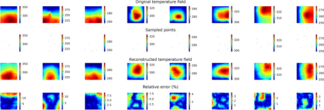
In Fig. 6 we show several results from the test dataset, for a random sampling method in the case where only 5 values are sampled, as it could occur in reality if it is difficult to place temperature sensors in the device to be monitored. From the Figure it can be clearly seen that the reconstruction accuracy is significantly degraded with respect to the example shown in Section “Results”; however it is still possible in this extreme case to obtain a qualitatively correct temperature in most cases.

Fig. 6.

Several examples of reconstructed temperature fields for the scattered sampling method in an extreme case where only 5 samples are taken. The rows are, from top to bottom, the ground truth temperature, the sampled temperature values, the reconstructed temperature field and the relative error in percent (see Eq. 2).

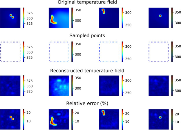
In Fig. 7 we show a few examples in which heat does not propagate through the system (due to the distribution of heat conductivity in those cases), resulting in very localized hot spots. Applying the Grid-edge (or the ring sampling method) the model does not have enough information to resolve such thermal distributions. Note that, for this kind of systems, the random sampling method renders significantly better results.

Fig. 7.

Several examples of systems with localized hot spots, for which our models cannot successfully reconstruct the temperature distribution. The rows are, from top to bottom, the ground truth temperature, the sampled temperature values, the reconstructed temperature field and the relative error in percent (see Eq. 2).

Experimental evaluation

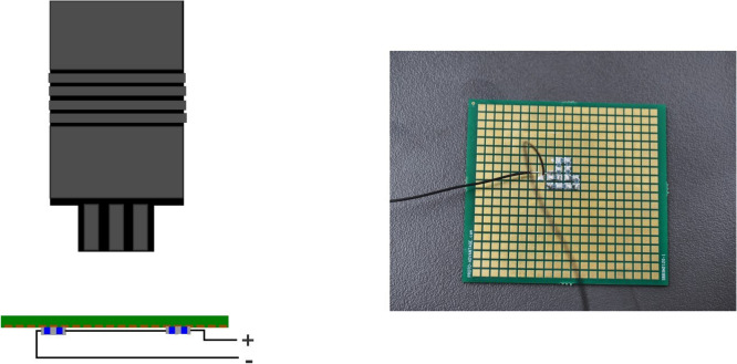
So as to evaluate the model’s effectiveness on physical data a simple experimental setup was chosen (see Fig. 8) to gather data for evaluation. We chose to use Surface Mounted Device (SMD) prototyping boards of a size as close to that of the generated samples as possible (53.3 mm $\times$ 58.4 mm), their construction consists of a single layer of FR4 1.6mm thick and 420 (2.0 mm $\times$ 2.0 mm)-square copper pads with a Electroless Nickel Immersion Gold finish placed in a grid pattern (21 rows $\times$ 20 columns).

Fig. 8.

Side view schematic of the thermal imaging setup with a VarioCAM®HD camera positioned to capture the temperature distribution of a PCB, which is illustrated with its electrical connections. Adjacent to this figure is an image showcasing the actual PCB used in the experiment.

In order to align physical measurements with those derived from simulations, Thermal Interface Materials (TIMs) were applied to the underside of some of the Printed Circuit Boards (PCBs). TIMs were specifically positioned over several copper pads to closely match the simulated thermal conductivities. This approach ensures that the experimental measurements are comparable to the generated data, facilitating a direct comparison between empirical observations and theoretical predictions.

SMD resistors were soldered onto the PCB’s pads in various patterns, an example PCB is shown in Fig. 8. The selection of these patterns was guided by the objective of ensuring comparability with simulation results.

The PCBs were clamped in a PCB soldering holder to secure them in place during data gathering and to have as little thermal conduction loss as possible. Power approaching the rated maximum of the resistors was then conducted through the resistor networks in order to heat them up, and after reaching steady state the thermal images where taken with an InfraTec VarioCam®HD and IR camera.

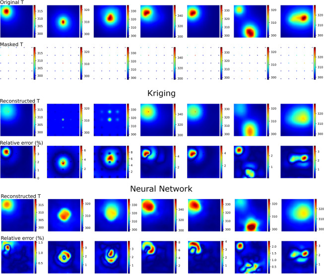
In this case we choose a regular sampling pattern for convenience, as shown in Fig. 9. The NN predictions are obtained by evaluating the NN models previously trained on 2D images for the scattered sampling method. As we see, even though in a 3D experimental scenario there are many effects not taken into account in the training of our 2D models, the temperature reconstruction is reasonably good. However, the description of the 3D experimental setup as a 2D system is a crude approximation which neglects heat dissipating normal to the large PCB surface, as well as radiation and convection effects. In the future we will develop models trained on 3D simulations including the 3D heat equation for training and allowing heat dissipation through all outer surfaces, and we expect these to perform even better for the experimental system than the current ones.

Fig. 9.

Comparison between Kriging and our neural network approach for several examples of reconstructed temperature fields from measurement data. A regular scattered sampling pattern is used. The rows are, from top to bottom, the ground truth temperature, the sampled temperature values, the reconstructed temperature field and the relative error in percent for the two different approaches respectively (see Eq. 2).

Comparison with Kriging

To evaluate the efficacy of our neural network-based approach for reconstructing temperature fields in a broader context, we conducted a comparative analysis against a conventional method widely recognized for spatial interpolation: Kriging. Kriging is a statistical technique that generates an estimated surface from a scattered set of points with known values, leveraging the spatial correlation between points to predict unknown values. This method assumes that the distance or directional variance between sample points reflects a spatial correlation that can be modeled, thus providing a means to interpolate data points across the domain. For the implementation of Kriging in our comparison, we utilized the Python library pykrige, specifically employing the UniversalKriging class with a Gaussian variogram model, using the default parameters.

The results for the reconstruction of the measured temperature fields with the Kriging algorithm and our neural-network-approach are shown in Fig. 9. Kriging generally leads to smoother temperature distributions - which visually appear more conformal to real temperature fields. There are, however, two major shortcomings which limit the applicability of Kriging in temperature monitoring scenarios. First, the maximum temperature is consistently underestimated. However, the maximum temperature and the temperature gradients are important monitoring features since they may lead to failure or degradation of the electronic components. These maximum temperatures are better captured by our NN-based approach. Second, the NN-based approach is more robust if the available measurement points contain little information. For instance, this is the case for the 2nd and 3rd system from the left in Fig. 9. For these systems, Kriging fails while the presented NN-based method still gives reasonable results. The reason is that the NN takes the statistics of the whole training dataset into account to produce the most likely temperature distribution, while the Kriging method is only relying on the available measurements of each individual system.

Scope of blind virtual sensing

It might seem implausible that the network can learn to reconstruct temperature distributions based on a few sensor points without knowing the material distribution in the system. It is clear that the difficulty of the virtual sensing problem depends on the sampling method. In principle, the material distribution could be inferred implicitly if enough sensor points are given (as can be argued for the regular grid sampling - see results in Fig. 3). In cases where this is not possible, e.g. when only points on the periphery are given as input, the network can only implicitly infer the most likely distribution of materials that best fits the few temperature sensors given and the statistics of the training dataset it has seen. We show many cases where this works reasonably well (Figs. 4 and 5) but also the key features where the method fails (hotspots in Fig. 7). To summarize, it has to be understood that the proposed method is not intended as a general-purpose tool to reconstruct the temperature field of any given system. However, in real-world applications some key features of the systems-of-interest are known, e.g. the range of material properties, the general structure of the system etc. Thus, the training dataset must be chosen carefully to represent these features, so that the network can learn the most likely temperature distribution from the dataset. In our case, the material properties are limited to the ranges specified in Table 1, and the geometry is constructed of squares of a given size range (see description in Section “Data generation”).

Conclusion

We have presented a model for the virtual sensing of thermal distributions using neural networks and for three different types of temperature sampling of the system. The average relative error in all cases presented is below $1.15\%$, even when noise is added to the samples to represent measurement errors in a real-world scenario. The model requires no information about the materials or heat source distribution inside the system for its predictions. The techniques presented in this work can also be used to find the optimal sampling for a given system, which will likely increase the temperature reconstruction accuracy.

As shown in Section “Extreme examples”, the model fails at identifying very small hot spots for the square and Grid-edge mask. Detection of hot spots is interesting in several applications, for example when virtual sensing is performed for state-of-health monitoring of a device. In our future work, we intend to improve the capabilities of our models in this regard.

Our model performs better than Kriging, which is a standard classical method for virtual sensing, as we show in Section “Comparison with Kriging”.

Finally, even though the models presented in this paper were trained for 2D systems, we show in Section “Experimental evaluation” that they perform reasonably well for real measurement data of the temperature of a PCB with SMD components.

All this makes us very confident that a future 3D version of our models will be a valuable addition to the toolbox for virtual sensing in electronic systems.

Author contributions

S.S. developed the code, wrote main parts of the manuscript text and prepared figures. H.S-A developed the code, evaluated the models, wrote main parts of the manuscript text, prepared figures. A.W. performed the experimental evaluation and contributed to its description in the manuscript text. J.R. performed the experimental evaluation and contributed to its description in the manuscript text. M.S. contributed to the model implementation, model evaluation and to the writing of the manuscript text.

Data availability

The datasets generated and analysed during the current study, as well as the code, are available in the temperature-reconstruction repository, https://opensource.silicon-austria.com/sabathiels/temperature-reconstruction

Declarations

Competing interests

The authors declare no competing interests.

References

- 1.Ahn, C.-U., Oh, S., Kim, H.-S., Park, D. I. & Kim, J.-G. Virtual thermal sensor for real-time monitoring of electronic packages in a totally enclosed system. IEEE Access10, 50589–50600. 10.1109/ACCESS.2022.3174208 (2022). [Google Scholar]
- 2.Liu, L., Kuo, S. M. & Zhou, M. Virtual sensing techniques and their applications. In 2009 International Conference on Networking, Sensing and Control, pp. 31–36, (IEEE, 2009).
- 3.Shao, W., Ge, Z., Yao, L. & Song, Z. Bayesian nonlinear Gaussian mixture regression and its application to virtual sensing for multimode industrial processes. In IEEE Transactions on Automation Science and Engineering, vol. 17, no. 2, pp. 871–885, (IEEE, 2019).
- 4.Kullaa, J. Bayesian virtual sensing in structural dynamics. In Mechanical Systems and Signal Processing, vol. 115, pp. 497–513, (Elsevier, 2019).
- 5.Wang, Y., Zhou, J., Ren, Q., Li, Y. & Su, D. 3-D steady heat conduction solver via deep learning. IEEE J. Multiscale Multiphys. Comput. Tech.6, 100–108 (2021). [Google Scholar]
- 6.Sanchez-Gonzalez, A., Godwin, J., Pfaff, T., Ying, R., Leskovec, J. & Battaglia, P.W. Learning to simulate complex physics with graph networks. In International Conference on Machine Learning, pp. 8459–8468, (2020).
- 7.Pfaff, T., Fortunato, M., Sanchez-Gonzalez, Al., Battaglia, P. W. Learning mesh-based simulation with graph networks. In NeurIPS, (2020).
- 8.Peng, J.-Z., Liu, X., Aubry, N., Chen, Z. & Wu, W.-T. Data-driven modeling of geometry-adaptive steady heat conduction based on convolutional neural networks. Case Stud. Thermal Eng.28, 101651. 10.1016/j.csite.2021.101651 (2021). [Google Scholar]
- 9.Wang, Y. & Ren, Q. A versatile inversion approach for space/temperature/time-related thermal conductivity via deep learning. Int. J. Heat Mass Transfer186, 122444. 10.1016/j.ijheatmasstransfer.2021.122444 (2022). [Google Scholar]
- 10.Raissi, M., Yazdani, A. & Karniadakis, G. E. Hidden fluid mechanics: Learning velocity and pressure fields from flow visualizations. In Science, vol. 367, pp. 1026–1030, (American Association for the Advancement of Science, 2020) 10.1126/science.aaw4741 [DOI] [PMC free article] [PubMed]
- 11.Pollok, S., Olden-Jørgensen, N., Jørgensen, P. S. & Bjørk, R. Magnetic field prediction using generative adversarial networks. J. Magn. Magn. Mater.571, 170556 (2023). [Google Scholar]
- 12.Zhao, X., Gong, Z., Zhang, Y., Yao, W. & Chen, X. Physics-informed convolutional neural networks for temperature field prediction of heat source layout without labeled data. Eng. Appl. AI117, 105516 (2023). [Google Scholar]
- 13.Manavi, S., Becker, T. & Fattahi, E. Enhanced surrogate modelling of heat conduction problems using physics-informed neural network framework. Int. Commun. Heat Mass Transfer142, 106662. 10.1016/j.icheatmasstransfer.2023.106662 (2023). [Google Scholar]
- 14.Raissi, M., Perdikaris, P. & Karniadakis, G. E. Physics-informed neural networks: A deep learning framework for solving forward and inverse problems involving nonlinear partial differential equations’’. J. Comput. Phys.378, 686–707. 10.1016/j.jcp.2018.10.045 (2019). [Google Scholar]
- 15.Karniadakis, G. E. et al. Physics-informed machine learning. Nat. Rev. Phys.3(6), 422–440. 10.1038/s42254-021-00314-5 (2021). [Google Scholar]
- 16.Go, M. S., Lim, J. H. & Lee, S. Physics-informed neural network-based surrogate model for a virtual thermal sensor with real-time simulation. Int. J. Heat Mass Transfer214, 124392. 10.1016/j.ijheatmasstransfer.2023.124392 (2023). [Google Scholar]
- 17.Stipsitz, M. & Sanchis-Alepuz, H. Approximating the full-field temperature evolution in 3D electronic systems from randomized ’Minecraft’ systems. arXiv preprint arXiv:2209.10369, (2022).
- 18.Sanchis-Alepuz, H. & Stipsitz, M. Towards Real Time Thermal Simulations for Design Optimization using Graph Neural Networks. In 2022 IEEE Design Methodologies Conference, DMC 2022, 10.1109/DMC55175.2022.9906469, (Institute of Electrical and Electronics Engineers Inc., 2022).
- 19.Stipsitz, M. & Sanchis-Alepuz, H. Approximating the steady-state temperature of 3d electronic systems with convolutional neural networks. Math. Comput. Appl.27(1), 7 (2022). [Google Scholar]
- 20.Geuzaine, Christophe & Remacle, Jean-François. Gmsh: A 3-D finite element mesh generator with built-in pre-and post-processing facilities. Int. J. Numer. Meth. Eng.79(11), 1309–1331 (2009). [Google Scholar]
- 21.Malinen, M. Elmer finite element solver for multiphysics and multiscale problems, (2013).
- 22.Ronneberger, O., Fischer, P. & Brox, T. U-net: Convolutional networks for biomedical image segmentation. In Medical Image Computing and Computer-Assisted Intervention–MICCAI 2015: 18th International Conference, Munich, Germany, October 5-9, 2015, proceedings, part III 18, pp. 234–241, Springer, (2015).
- 23.Harutyunyan, H., Reing, K., Ver Steeg, G. & Galstyan, A. Improving generalization by controlling label-noise information in neural network weights. In International Conference on Machine Learning, pp. 4071–4081, (PMLR, 2020).
Associated Data
This section collects any data citations, data availability statements, or supplementary materials included in this article.
Data Availability Statement