Length-scale study in deep learning prediction for non-small cell lung cancer brain metastasis

Abstract

Deep learning-assisted digital pathology has demonstrated the potential to profoundly impact clinical practice, even surpassing human pathologists in performance. However, as deep neural network (DNN) architectures grow in size and complexity, their explainability decreases, posing challenges in interpreting pathology features for broader clinical insights into physiological diseases. To better assess the interpretability of digital microscopic images and guide future microscopic system design, we developed a novel method to study the predictive feature length-scale that underpins a DNN’s predictive power. We applied this method to analyze a DNN’s capability in predicting brain metastasis from early-stage non-small-cell lung cancer biopsy slides. This study quantifies DNN’s attention for brain metastasis prediction, targeting features at both the cellular scale and tissue scale in H&E-stained histological whole slide images. At the cellular scale, the predictive power of DNNs progressively increases with higher resolution and significantly decreases when the resolvable feature length exceeds 5 microns. Additionally, DNN uses more macro-scale features associated with tissue architecture and is optimized when assessing visual fields greater than 41 microns. Our study computes the length-scale requirements for optimal DNN learning on digital whole-slide microscopic images, holding the promise to guide future optical microscope designs in pathology applications and facilitating downstream deep learning analysis.

Introduction

The use of deep neural networks (DNN) applied to digitized histopathology images has increasing importance in both biomedical research and clinical practice^1,2. Novel imaging techniques and DNN analyses are already simplifying laborious tasks associated with routine pathological assessment^3,4. More intriguingly, these same DNN approaches can also formulate clinical outcome predictions based on subtle image features, which surpasses the ability of human pathologists and even elutes human interpretation^5–7. However, DNN-based analysis systems that can accurately perform these tasks are proportionally larger and more complex. This further restricts our ability to understand the basis of AI-identified histopathology features that may provide physiological disease insights (i.e. ‘explainability’). At the same time, critical measurement parameters that are best suited for optical DNN processing and analysis are not well understood.

To improve interpretability, numerous novel approaches have been developed and evaluated in recent years^8–11. Saliency maps or class activation maps can be computed to visualize the attention of DNN from backpropagating the model weights^12–15. The intuition behind this type of method is that the change in the DNN output can be traced back to the individual perturbations of the pixel values in the images. These methods can highlight where the DNN is focusing and give humans a sense of which part might be more important within the image. A second group of saliency mapping methods is based on occluding some parts of the images and checking the resulting variation in DNN outputs^16,17. Similarly, occlusion maps can be generated to track DNN’s attention. The third category of methods is to visualize the digital filters in different layers of DNNs^18–20. In medical image analysis, other explainable models have been developed such as concept learning models^21–23 and case-based models^24,25. The concept learning models predict high-level clinical features first, and then make final decisions based on these clinical features. Case-based models make predictions by comparing the latent space features extracted from an input image against class discriminative prototypes. The methods mentioned above have achieved significant advances in explaining DNN for human-understandable tasks, such as image classifications^15,26, tissue or cell segmentation²⁷, and auto-pilot of self-driving systems²⁸.

Recently, a few studies have investigated the effect of image resolution and field of view in different deep learning tasks. A few studies were focused on developing new deep learning pipelines for finding the optimal tile size^29,30. However, these studies did not investigate how the change of minimally resolvable features and maximum physical image size affected the DNNs’ performance. In other studies, researchers evaluated the effect of image resolution or image physical size in deep learning tasks. For example, researchers studied DNN performance variations while degrading the image resolution without reducing the image physical size in radiography³¹. However, this work was focused on finding the optimal range of tile sizes for DNN analysis. In another study, researchers focused on finding the optimal image size for cancer tumor detection with a convolutional neural network³². Our study differs from these studies in that we are not trying to optimize DNN performance, and instead, are focused on uncovering characteristic length scales associated with the disease under study.

In this paper, we introduce a new method for shedding light on the prediction mechanism in image-based DNN analysis and bringing in new understandings of image requirements for microscopic imaging system designs. This approach operates by altering the image resolution and field-of-views of the training and testing image data and studying the impact on DNN prediction accuracy to identify the length-scale that optimizes DNN learning. This generalized approach can apply to all DNN architecture, as it is network agnostic. In the application of digital pathology analysis, it provides length-scale information about the DNN’s predictive ability which can be used to optimize that ability and that a human pathologist can in turn use to better understand predictive physiological features. Compared to existing model interpretation methods, which generally assess a model’s parameters gradient in order to generate attention maps, our method gradually degrades the information content of the input data in order to discover vital length scales associated with disease prediction, and does not require access to the internal DNN parameters to generate attention maps. Additionally, the feedback on the different levels of the length-scale provides the features’ significance at different optical resolutions. This can potentially facilitate microscope design enabling the trade-offs among optical resolutions, imaging speed, pixel sampling requirements, etc.

Here, we demonstrate the use of this method on a DNN that has been trained to predict brain metastasis in early-stage non-small-cell lung cancer (NSCLC) subjects through high-quality whole slide images (WSI) of the diagnostic pathology slides. For context, we note that NSCLC is one of the most lethal cancers globally. Nearly a third of early-stage (Stage I-III) cases will recur with distant metastases³³, and brain metastasis is a common cause of morbidity and mortality in NSCLC³⁴. At present, it is not possible to accurately predict the metastatic potential of NSCLC using conventional histopathological analysis, even when supplemented with genomic or molecular biomarkers³⁵. This limitation is especially significant for patients diagnosed at an early stage, where precise risk assessment plays a pivotal role in making treatment decisions. Recently, we developed and trained a DNN to predict brain metastasis using diagnostic WSI⁵. While this DNN is capable of making meaningful and statistically significant predictions, it shares the opacity associated with most other related image analysis DNN – thus making it an excellent candidate for this length-scale study method.

The length-scale study is composed of training and testing the same DNN for different resolvable feature lengths (RFLs) and maximum feature lengths (MFLs) of the input images. The detailed definition of RFL and MFL will be introduced in the Material and Methods section. The RFLs reveal feature detail length-scale that is important to the DNN predictive ability, while the MFLs reveal how distance and large-scale features contribute to the DNN outcome.

Material and methods

This study is based on our recent demonstration that DNN on WSI from patients with early-stage NSCLC can reliably predict which cases progressed to brain metastases and those that had no recurrence of any type after extended follow-up⁵. The current study uses the same WSI to investigate features necessary to optimize the prediction potential of DNN.

Ethics statement

All procedures related to this study were conducted under an Institutional Review Board-approved protocol, which allowed for the selection of tissue blocks and slides from pre-existing institutional diagnostic material, linkage to non-identifying, limited clinical datasets (where available), and de-identification of all images through an ‘honest broker’ mechanism. All data related to this study is publicly available at CaltechData (https://doi.org/10.22002/dw66e-mbs82), and all images are de-identified.

Patient cohort

A cohort of treatment-naïve 158 patient cases were recruited in this study with early-stage (Stage I-III) NSCLC diagnosed and treated at Washington University School of Medicine with long-term follow-up (>5 years or until metastasis). In total, 158 fresh Hematoxylin and Eosin (H&E) stained slides were retrieved and processed from existing, de-identified formalin-fixed paraffin-embedded (FFPE) diagnostic tissue blocks and imaged by an Aperio/Leica AT2 slide scanner (Leica Biosystems, Deer Park, IL, USA) including a 20$\times$/0.75 NA Plan Apo objective lens and a 2$\times$ magnification changer. The 158 cases were categorized into two groups, Met+: 65 cases with known brain metastasis, and Met-: 93 cases with no recurrence after extended follow-up. The median follow-up time of this cohort was 12.2 months and 106 months for Met+ and Met- groups, respectively.

General deep learning pipeline

The scanned 158 whole slide images were first reviewed by a pathologist. The primary tumor regions with their tumor micro-environment were roughly annotated (Fig. 1a). The annotation to demarcate the primary tumor and related regions was done on a slide level. Additionally, the Ostu thresholding³⁶ was performed at the annotated regions to remove the backgrounds (plain glass). We then randomly sampled image tiles from the annotated regions and cellular content related in the subsequent steps. This ensured that the tiles were representative of the histological features in the dataset. A thousand non-overlapping image tiles for every whole slide image were randomly selected to undergo a color normalization process³⁷, which are then taken as the inputs for the DNN. The classification ground truth labels in the supervised learning were given by the metastatic progression outcome of each patient/slide. In other words, the task was weakly supervised by slide-level/patient-level ground truth labels.

Fig. 1.

(a) Preprocessing pipeline of H&E-stained whole slide images. The whole slide image is manually annotated by a human expert. The annotation mask is processed with thresholding to get rid of the background region. A thousand non-overlapping image tiles are randomly selected from the masked region. (b) One experiment of training-testing split in deep learning pipeline. Acc. stands for “accuracy”.

The ResNet-18³⁸ convolutional neural network pretrained on the ImageNet dataset was used as the backbone in our DNN structure. The linear layers in the DNN were replaced by a linear layer and a sigmoid activation layer to adapt our binary classification task. For every input image tile, the model outputs an individual score—a prediction score. This tile-level score is supervised by the binary-encoded label from Met+ and Met-.

In clinical deep learning studies, due to a lack of well-established testing sets, multiple training-testing splits are usually adopted to avoid potential bias in the testing set selection from a single experiment. As illustrated in Fig. 1b, we designed three individual experiments with different training-testing splits. Each of the training sets had 118 cases (Met+: n=45, Met-: n=73) and each of the testing sets had 40 cases (Met+: n=20, Met-: n=20), with 1000 image tiles per case. We chose to use 1000 image patches based on our prior study where we had varied the number of patches from 100 to 3000 and found that the model performance stability required 1000 or more image patches with different random seeds⁵. Note that the mild imbalanced training dataset effect was mitigated by using a large batch size with 200 image tiles in each batch³⁹. Therefore, in each gradient descent iteration, the model saw adequate samples in both Met+ and Met-. Also, the standard data augmentations, including random crop, random rotation, and random flipping, are implemented during the training process. Dataset imbalance is a common situation in machine learning, and the protocols for addressing it are common and numerous^39–44. The training-testing splits were done with randomization and the three testing sets had no overlapping patients. Finally, the performance of the classifier is evaluated by the tile-level accuracies.

Length-scale definition and investigation

The RFL is the minimum feature length that can be resolved in the input image. This feature length is constrained by the Nyquist-Shannon sampling theorem in the digital image⁴⁵. For example, suppose the input image has a pixel count of 224-by-224 pixels with a pixel pitch of 0.51 microns. According to the Nyquist-Shannon sampling theorem, the minimum resolvable feature requires at least two pixels in image sampling along each of the lateral axes. In this case, our RFL would be 1.02 microns which is twice the pixel pitch. In this example, the RFL matches the physical resolution limit of the microscope used to acquire this image. By down-sampling the image while maintaining the same tile size, we can generate images that are more poorly resolved and thus have larger RFL. RFL can alternately be interpreted as the image resolution – we avoided using the term ‘resolution’ here because resolution generally refers to one of the imaging system specifications, while we use RFL here to refer to the target sample intrinsic feature length-scales.

Our study involves performing a sequence of down-sampling to the base image data set in order to generate data sets with varying RFL. As a technical note, we note that to avoid passing tiles of different pixel counts to the DNN and complicating the comparison process, the image tiles are interpolated after down-sampling to maintain the same overall pixel counts.

The MFL is associated with the input image field-of-view, which is defined by the physical size of the input digital image tile. Specifically, the MFL is confined by the images’ physical range – the size of the image in microns or the lateral extent of the image field-of-view. Once again, we can use the input image with a pixel count of 224-by-224 pixels and a pixel pitch of 0.51 microns as an example. In this case, the MFL would be 114 microns, which is given by the product of 224 pixels and 0.51 microns pixel size. We can generate data sets with smaller MFLs by using smaller tile sizes. As a technical note, we again note that to avoid passing tiles of different pixel counts to the DNN and complicating the comparison process, the image tiles are interpolated after down-sampling to maintain the same overall pixel counts.

The length-scale study was conducted under different RFLs and distinctive MFLs for the input image tiles (Fig. 2). For RFLs, the image tiles were resampled with fewer pixels in rows and columns and then interpolated back to the original size. After operating this process, the detailed features of the image contents were removed. For different MFLs, the image tiles were cropped to smaller sizes and then interpolated back to the original size to meet the input size requirement from DNN. In this process, the distant features or large-scale features were blocked out before feeding into the DNN. The combination of these two processes can reveal contributions from various levels of the features. For every RFL or MFL, the deep learning pipeline described in the General deep learning pipeline section was performed. To guarantee the consistency of our experiments, the number of image tiles for training models at each MFL or RFL are the same and are from the same non-overlapping regions in the whole slide images. The cropping process in the MFL analysis consistently crops the image patch from the center of the original image tile. This patch gets smaller as the MFL decreases, but it is always from the center of the original image tile. The results and interpretations will be discussed in the Results section.

Fig. 2.

A schematic diagram of the length-scale processing pipeline for (a) RFL and (b) MFL. The red arrows indicate the training flow, and the green arrows denote the testing flow. The black dashed line is associated with a specific length-scale data input. The different levels of the length-scales are obtained by information attrition from downsampling or cropping the input images. Acc. stands for accuracy.The experimentally derived accuracy-versus-RFL and -MFL curves are shown in detail in Fig. 3.

Piecewise linear fitting and slope maps

To further facilitate the usage of length-scales and exploit the information encoded in MFLs and RFLs, we first performed a piecewise linear fitting to find the range of length-scales of significant interest. Then, we computed slope maps to visualize the model’s attention and reveal the effect of information attrition on the input data. A piecewise linear fitting or a linear fitting was performed on the prediction outcomes at a tile level from distinct MFLs or RFLs. We note that performing linear fitting on tile-level prediction outcomes can benefit the computation of slope maps, as discussed in the next paragraph. The determination of single-step or two-step linear fitting depended upon the fitting errors. We minimized the fitting errors and found the optimal fitting representations for the length-scales.

The slopes of the linear-fitted lines for each RFL and MFL length scale plot are proportional to the effect that input information degradation has on the DNN’s prediction accuracy. To better understand how this degradation affects the spatial distribution of the DNN’s attention, we computed the slope values across the greatest change effected by length-scale range in each tile and mapped those values to the corresponding spatial locations on the whole slide image. For visualization purposes, the slope values are normalized between -1 and 1. A positive slope value denotes a degradation of prediction outcome accuracy corresponding to an image tile where there was a loss of information during the change of length-scale. In contrast, a negative slope value indicates an actual improvement of prediction outcome accuracy corresponding to an image tile where there was a loss of information during the change of length-scale. In this way, the slope maps can reveal the effect of model behaviors on spatial analyses and contributing histological features.

Note that we use accuracy as the classification performance metric throughout this paper because our test set is balanced. As such, accuracy is a convenient and appropriate metric. In principle, another classification performance metric, such as F1-score could be used as well, because our proposed method is primarily interested in the relative change in accuracy (or any other accuracy metric, such as F1-score) as spatial information is gradually degraded, rather than the absolute accuracy value (Supplementary file 1).

Results

Length-scale for early-stage NSCLC metastasis prediction

The initial pilot study was designed to check the feasibility of DNN in predicting brain metastasis⁵. Though brain metastasis occurs frequently in NSCLC, no clinically effective predictor has been reported, to the best of our knowledge, particularly in early-stage (Stage I-III) NSCLC^35,46. Our pilot study DNN was trained on the patient cohort with well-defined and clinically relevant endpoints (Met+ versus Met-). The DNN was then evaluated on three training-testing experiments.

By preserving the designed architecture of DNN, we conducted a length-scale study that included a sub-study on the RFL and a sub-study on the MFL. For the RFL sub-study, we down-sampled the input image tiles from 1 to 30 in 18 levels and compared them to their original size, which corresponds to the RFL range of 1.02 microns (the sharpest resolution we could obtain) to 31 microns. Image tiles at each RFL value underwent the three-fold training-testing procedure described in the General deep learning pipeline section. The average achieved accuracy for the experiments versus RFL is plotted in Fig. 3a. For the MFL sub-study, we prepared 12 data sets with MFL ranging from 2.5 to 114 microns. The image tiles at each MFL value underwent the same three-fold training-testing procedure described in the General deep learning pipeline section. The average achieved accuracy for the experiments versus MFL is plotted in Fig. 3b.

Fig. 3.

Length-scale study curves for different (a) RFLs and (b) MFLs. The dotted arrow at the top indicates the length-scale from small size to large size. The black solid lines are the piecewise linear fittings to the average values of the three experiments. The “+” marker indicates the result from the original study⁵.

The leftmost points in Fig. 3a are the same as the rightmost points in Fig. 3b, representing the prediction accuracy of the DNN on unmodified tiles in original studies. As we degrade the information content of the tiles (either by increasing RFL or decreasing MFL), the prediction accuracies decline in the figures. These reductions may be due to different mechanisms of information loss associated with RFL and MFL.

The average values of the three experiments in Fig. 3 were fitted with piecewise linear functions with different slopes and intercepts, which exhibits a smaller fitting error compared to regular linear fitting. The variations in tile-level accuracy changes across RFLs and MFLs indicated that distinctive length-scales contribute differently to the overall accuracies. We noticed that when we significantly increased RFL or reduced MFL, the accuracy did not drop to 50% as a random guess in binary classification. This suggests that the color or staining of these H&E images likely has a slight impact on the predictivity of brain metastasis.

The curves for accuracy versus RFL underwent a relatively rapid drop before leveling out. The transition point was determined to be at an RFL of 5.1 microns— for ease of reference, we will label this as the characteristic RFL. This transition point was determined by minimizing the absolute residue error from the piecewise linear regression. The sharp drop-off in prediction accuracy before the characteristic RFL suggests that the DNN’s predictive capability is most sensitively associated with length-scale features smaller than 5.1 microns. As can be seen in Fig. 3a, the accuracy markedly improves as length scale features become progressively smaller (i.e., progressively achieve higher visual resolution between 5.1 microns and 1.02 microns (maximal resolution). That is, the higher the resolution of the image, the greater the prediction accuracy. This result also suggests that if we could have obtained a smaller RFL, by for example scanning at higher power, even greater accuracy could have been achieved.

Figure 4 visually illustrates the features of interest. The left column shows representative vignettes of the original images at maximal resolution, that is RFL of 1.02 microns. The middle column shows the same vignettes with features of length-scale smaller than 5.1 microns removed. The differences between the two columns are shown in the right column. From Fig. 4, we can appreciate the type of visual data that DNN depends on for its prediction. Particularly notable here is that in while color information is preserved (which as mentioned earlier clearly carries information used by the DNN in its predictive algorithm), the architectural and cellular information is largely lost at RFL >5.1 microns.

Fig. 4.

Visualization of (a) original image patches, (b) images at $\text{RFL}=5.1\mathrm{\mu }\text{m}$, and (c) the subtraction of (a) and (b). Note that while color information is preserved, the architectural and cellular information is largely lost at RFL 5.1 microns, as demonstrated by the preservation of these features in the subtraction images.

Our MFL analysis shows a prediction accuracy transition as well. The curves for accuracy versus MFL underwent a transition at MFL of 41 microns – for ease of reference, we will label this as the characteristic MFL. This transition point was determined by minimizing the absolute residue error from the piecewise linear regression. This characteristic MFL indicates that the DNN is not simply focused on single cells (average size of 8 microns) for its prediction but instead appears to use stromal content and/or the inter-relationship between cells as well. As the MFL increases from 41 to 114 microns, there is a slight increase in information accuracy, approaching 80% at 114 microns. However, that increase is modest.

Taken together, these two sub-studies indicate that the DNN derives its predictive power from both sub-cellular content information and tissue-level content information. Neither set of information on its own is sufficient for DNN to obtain optimal predictive accuracy. These data suggest that, in the context of the current study parameters, the majority of information content relevant to DNN for prediction lies within RFL (resolution) of <1.02 microns and MFL (field-of-view) >41 microns). The data also strongly suggest that if we had been able to achieve an even higher RFL, that is <1.02 microns (which would be possible by scanning the slides at higher power), we could have achieved even higher DNN predictive accuracy.

Histological analysis of DNN’s attention

This length-scale analysis can be used to further facilitate an understanding of DNN attention across the whole-slide images. To visualize the DNN attention across the whole slide image, we can produce slope maps through our RFL and MFL DNNs, as described in the piecewise linear fitting and slope maps subsection. We applied this slope analysis approach to two slides from our data set. The results are presented in Fig. 5 (Met+ case) and Fig. 7 (Met- case), both correctly predicted by the DNN. Figures 5 and 7 (a-c) are a) the whole slide image, b) the processed annotation mask and c) the corresponding primary tumor region. In the slope maps based on RFL (Figs. 5d and 7d) and MFL (Figs. 5e and 7e) the warm (orange) color indicates tiles where the DNN prediction was accurate and sensitive to either RFL or MFL (Figs. 5d and 5e respectively), while cool (blue) color indicates tiles where the wrong prediction was made on that tile. Tiles with no color indicate areas where the DNN did not make a meaningful prediction and the prediction was insensitive to either RFL or MFL.

Fig. 5.

(a) Whole slide image of a Met+ case. (b) Processed annotation mask. (c) Annotated H&E section. Slope maps for individual tiles examining the role of (d) RFLs and (e) MFLs, where orange indicates tiles where the DNN prediction for that tile was accurate, while blue indicating tiles were incorrect prediction. Zoom-in images in (d) and (e) the orange and blue boxes showing the same tissue area for RFL (d) and MFL (e).

Fig. 7.

(a) Whole slide image of a Met- case. (b) Processed annotation mask. (c) Annotated H&E section. Slope maps for individual tiles examining the role of (d) RFLs and (e) MFLs, where orange indicates tiles where the DNN prediction for that tile was accurate, while blue indicating tiles were incorrect prediction. Zoom-in images in (d) and (e) the orange and blue boxes showing the same tissue area for RFL (d) and MFL (e).

The blue-colored tiles deserve some elaboration. For these tiles, the trained DNN actually made the wrong prediction on the tiles but made the correct prediction at the slide level. This dichotomy can be understood that as we begin to drop out image information (by increasing RFL or decreasing MFL), the trained DNN’s prediction for a given tile began to asymptote towards a random guess prediction, which is on average closer to a correct prediction.

At the slide level, we can analyze the histologic features of the tiles demonstrating accurate prediction and sensitivity to changes in RFL and MFL (Figs. 6a and 8a) versus where the DNN did not make a meaningful prediction or an inaccurate prediction (Fig. 6b and 8b). For the tiles, the DNN was sensitive to changes in RFL and MFL and accurately predicted metastasis (Fig. 6a) or accurately predicted no metastasis (Fig. 8a), it can easily be seen that these tiles contain tumor and surrounding tumor microenvironment. In contrast, the histology seen in the tiles with no information for the DNN (i.e. where the DNN did not make a meaningful prediction or made an inaccurate prediction and was insensitive to changes in RFL and MFL, Figs. 6b and 8b) was very different; in these tiles, very little to no tumor or tumor microenvironment is seen, instead showing benign tissue composed of fibrosis, anthracitic pigment deposition, alveolar wall, fibroelastic tissue, pulmonary macrophages and/or reactive type pneumocytes.

Fig. 6.

Representative histologic images of tiles where (a) the DNN made an accurate prediction, while (b) the DNN made no prediction or an inaccurate prediction. In (a), note areas of tumor (black arrows) and tumor microenvironment including immune cells and desmoplastic stroma (blue arrows). In (b) note that there are reactive pneumocytes, pulmonary macrophages and alveolar wall (green arrows), and fibrosis (red arrows). We refer the readers to the Histological analysis of DNN’s attention subsection in the paper for a detailed description of relevant observations.

Fig. 8.

Representative histologic images of tiles where (a) the DNN made an accurate prediction and (b) made an inaccurate prediction. In (a), note areas of tumor (black arrows) and tumor microenvironment including immune cells and desmoplastic stroma (blue arrows). In (b) note that there is fibrosis and deposits of anthracitic pigment (red arrows) but no tumor cells. We refer the readers to the Histological analysis of DNN’s attention subsection in the paper for a detailed description of relevant observations.

Beyond providing insights at the whole-slide level and image tile-level, the length-scale analysis method can also be applied to regional image patches, for example, patches comprised of concatenation of 5-by-5 image tiles. Broadly speaking, analysis of this sort reinforces the idea that the DNN focuses on areas with tumors and that both increasing the RFL and decreasing the MFL negatively impact the ability of the DNN to correctly predict brain metastasis. For the more pathology-specialized readers, the details of our findings are as follow. Using the slope maps, to take into account even wider tissue area than 41 microns we selected examples of regions with low and high RFL and MFL sensitivity (Figs. 9 and 10). These are the same slide cases as Figs. 5 and 7, respectively. In this analysis, we concatenated 5-by-5 adjacent image tiles on the cases demonstrated in Figs. 5 and 7 in areas showing high predictive accuracy and high RFL and MFL sensitivity vs areas showing low predictive accuracy and low sensitivity to RFL and MFL (Fig. 9, Met+ and Fig. 10, Met-). Figures 9a and b and 10a and b demonstrate the histologic findings in Met+ and Met- cases where the individual tiles demonstrated accurate prediction and sensitivity to RFL (Figs. 9a2,b2 and Figs. 10a2,b2) and MFL (Figs. 9a3,b3 and Figs. 10a3,b3). The histology of these overall areas (Figs. 9a1,b1 and 10a1,b1) demonstrates clear tumor and peri-tumoral/tumor microenvironment, including desmoplastic stroma and infiltrating immune cells. In contrast, the areas where the concatenated tiles showed little prediction accuracy and insensitivity to RFL (Figs. 9c2,d2 and 10c2,d2) and MFL (Figs. 9c3,d3 and 10c3,d3) demonstrate an overall histology largely devoid of tumor cells and tumor stroma/microenvironment, consisting mainly of benign tissue including fibrosis, alveoli, reactive pneumocytes and macrophages (Figs. 9c1,d1 and 10c1,d1).

Fig. 9.

(a–d) Concatenation of 5-by-5 image tiles from Met+ case in Fig. 5. Areas a1 and b1 are the histology from a concatenated area where the DNN prediction was accurate and sensitive to changes in RFL (a2,b2) and MFL (a3,b3). Areas c1 and d1 are the histology from a concatenated area where the DNN prediction was low or inaccurate and insensitive to changes in RFL (c2,d2) and MFL (c3,d3). The color scheme is similar to Fig. 6. In a1 and b1, note areas of tumor cells (black arrows) and tumor microenvironment including immune cells and desmoplastic stroma (blue arrows). In c1 and d1, note that the tissue is largely devoid of tumor cells.

Fig. 10.

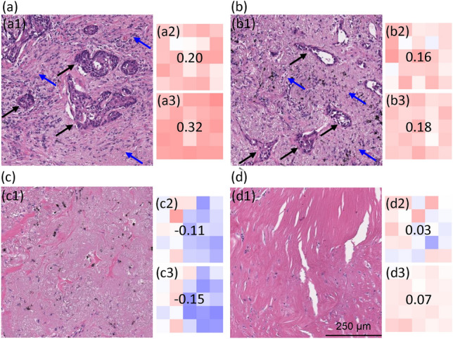
(a–d) Concatenation of 5-by-5 image tiles from Met- case in Fig. 7. Areas a1 and b1 are the histology from a concatenated area where the DNN prediction was accurate and sensitive to changes in RFL (a2,b2) and MFL (a3,b3). Areas c1 and d1 are the histology from a concatenated area where the DNN prediction was low or inaccurate and insensitive to changes in RFL (c2,d2) and MFL (c3,d3). The color scheme is similar to Fig. 8. In a1 and b1, note areas of tumor cells (black arrows) and tumor microenvironment including immune cells and desmoplastic stroma (blue arrows). In c1 and d1, note that the tissue is largely devoid of tumor cells.

Discussion

In this work, we present a method for assessing the parameters necessary to optimize DNN by analyzing the feature length-scale sensitivity of a trained image analysis DNN. Specifically, we examined the role of resolution (i.e. small sub-cellular scale features) via RFL and the role of more macro multi-cellular/tissue scale features via MFL. Using this approach, we examined a DNN algorithm that had been trained and validated to predict the future occurrence of brain metastases, or no metastases after long-term follow-up, in patients with early-stage (Stage I, II and III) NSCLC, based on DNN learning on the original H&E-stained slides of the diagnostic biopsies from these patients⁵.

Several interesting features are observed. It is clear that the higher the resolution (that is, the smaller the RFL), the greater the accuracy of the DNN algorithm. This also indicates building a high-resolution whole slide scanner is in need. In addition, we have also shown that a more macroscopic/multicellular tissue-based assessment (that is, larger MFL) is also crucial to DNN predictive capability. This indicates that not only is the AI using tumor cells to make its prediction, but is also using surrounding cells of the tumor microenvironment (TME), such as immune and stromal cells, to predict outcomes. This is perhaps unsurprising, given the increasing evidence of the role of TME in tumor progression^47,48. The observation that the higher resolving power (that is smaller RFL) than was possible in the current data set would result in even greater predictive accuracy strongly suggests that parameters could be optimized in future AI/DNN analysis of digital images, including capturing images at higher optical resolution. In any event, our study shows that it is a combination of sub-cellular and macro-cellular features that are important in DNN learning.

The findings point directions for brightfield microscope designs. To meet the demanding requirements of data-hungry tasks in deep learning, high optical resolution is of great importance by revealing all the subtle cellular details and interactions in the pathology slides. Ptychography^49,50 and Fourier Ptychographic Microscope (FPM)^51,52 can be potential alternative imaging techniques for whole slide imaging in pathology applications with fast imaging performance and high-quality image reconstructions^53,54. Especially for FPM, it is capable of imaging with large field-of-views and high resolutions simultaneously, which can be a good candidate to satisfy the requirements for deep learning study as discovered in this work.

We have also observed, in this study and previously⁵, that as we segment the DNN learning to small (tile) areas of defined pixel quantity, not all areas provide equal or even useful information. Indeed, in some cases, this tile-based analysis shows areas where the DNN prediction based on that area is the opposite to the overall prediction, and the opposite to truth. In order to further assess this, we compared the histology of the areas that showed high sensitivity to the effects of RFL and MFL and provided predictive accuracy with areas that were insensitive to RFL and MFL and provided no or even negative predictive accuracy. Our analysis demonstrates that the histology features of these areas are quite distinct; the histology of the highly sensitive and predictive areas show tumor cells in association with tumor microenvironment, such as infiltrating immune (lymphoid) cells and desmoplastic response (which is a reaction that is highly specific for tumor growth^55–57), and this is seen in the predictive areas in tumors where the DNN predicted no metastasis (and was correct) as well as in tumors where the DNN predicted the subsequent occurrence of brain metastases (and was correct). In contrast, the sub-areas in tumors that showed no or negative predictive value, but for which, at the slide level, the DNN correctly predicted the outcome for that patient (either the development of metastases or no metastases), sub-areas were virtually devoid of tumor and elements of the tumor microenvironment, instead showing fibrosis, anthracosis, alveolar wall, pulmonary macrophages, and reactive type pneumocytes. It is also notable that the areas showing high predictive value and sensitivity to RFL and MFL largely overlap and demonstrate tumor cells and tumor microenvironment, while the areas showing low or negative predictive value and low sensitivity to RFL and MFL similarly overlap and show no (or very few) tumor cells or tumor microenvironment. This clearly demonstrates that the presence of tumors is (not surprisingly) crucial in establishing a predictive DNN algorithm assessing tumor progression. What is perhaps more instructive is that tumor cells are not the only crucial feature, and elements of the tumor microenvironment appear to be independently important in establishing the predictive potential of the algorithm. We expect these observations to take on increasing importance as we dissect the biological basis for the ability of DNN to predict outcomes based on a digital image. Meanwhile, the current approach has its limitations in terms of its computational load. To obtain characteristic length-scale values or length-scale of interest, we need to apply the model training multiple times. This can be time-consuming and computationally heavy, especially when the dataset is large. In addition, for different tasks and datasets, the approach needs to be performed repeatedly. To broaden the technique for large datasets and types of tasks, more research would need to be done to investigate ways to jointly optimize different length-scale training efficiently.

In the broader context, for predictive tasks that are difficult/impossible for human experts to perform, but that deep learning/AI methods have demonstrated predictive value, we expect our method can help shed light on how different scales of features contribute to the model predictions. In this study, we demonstrated the application to the analysis of an NSCLC biopsy study with ResNet model, but the approach is not restricted to a specific disease type or model type. As our approach operates by gradually attriting the information content of the input data and examining the impact on the prediction accuracy, we can expect the approach to be readily adaptable to work on other AI models in other disease contexts. In this context, we may expect that specific characteristic length scales associated with different diseases could be different. For example, chronic diseases, such as diabetes, that have broader systemic impacts but that alter individual cell morphology minimally may have a different characteristic RFL value and/or MFL value. A follow-up study using the characteristic length scale approach to uncover the RFL and MFL length-scales associated with different diseases may provide interesting insights into the biology of those diseases. Finally, this study could contribute to the rational design of future studies to apply deep learning/AI to digital histopathologic images, including guidance on techniques of image acquisition and field-of-view metrics. The above speculations and anticipated outcomes would require further studies to confirm or uncover. In the future, we will investigate the approach application to broader scenarios, and we will also work to build a larger early-stage NSCLC dataset with metastatic clinical outcomes and multi-institutional collaboration to further validate the characteristic length-scale conclusions in the paper.

Author contributions

C.Y. and R.J.C conceived the idea, designed the experiments, and supervised the entire project. H.Z. and S.L. conducted all experiments and analyses. M.W. and R.G. prepared the experimental data. C.T.B. performed pathology analysis. O.Z. guided image analysis. L.L. contributed to the revision of the manuscript. All authors contributed to the writing and preparation of the manuscript.

Data availibility

The data is available at CaltechData https://doi.org/10.22002/dw66e-mbs82. The code⁵ is available at Github https://github.com/hwzhou2020/NSCLC_ResNet and https://github.com/hwzhou2020/NSCLC_length_scale.

Declarations

Compteting interest

The authors declare no competing interests.

Supplementary Information

The online version contains supplementary material available at 10.1038/s41598-024-73428-2.

References

- 1.Janowczyk, A. & Madabhushi, A. Deep learning for digital pathology image analysis: A comprehensive tutorial with selected use cases. J. Pathol. Inform.7, 29. 10.4103/2153-3539.186902 (2016). [DOI] [PMC free article] [PubMed] [Google Scholar]
- 2.Baxi, V., Edwards, R., Montalto, M. & Saha, S. Digital pathology and artificial intelligence in translational medicine and clinical practice. Mod. Pathol.35, 23–32. 10.1038/s41379-021-00919-2 (2022). [DOI] [PMC free article] [PubMed] [Google Scholar]
- 3.Shen, C. et al. Automatic detection of circulating tumor cells and cancer associated fibroblasts using deep learning. Sci. Rep.13, 5708. 10.1038/s41598-023-32955-0 (2023). [DOI] [PMC free article] [PubMed] [Google Scholar]
- 4.Falk, T. et al. U-Net: Deep learning for cell counting, detection, and morphometry. Nat. Methods16, 67–70. 10.1038/s41592-018-0261-2 (2019). [DOI] [PubMed] [Google Scholar]
- 5.Zhou, H. et al. Ai-guided histopathology predicts brain metastasis in lung cancer patients. J. Pathol.263, 89–98. 10.1002/path.6263 (2024). [DOI] [PMC free article] [PubMed] [Google Scholar]
- 6.Lu, M. Y. et al. A visual-language foundation model for computational pathology. Nat. Med.30, 863–874 (2024). [DOI] [PMC free article] [PubMed] [Google Scholar]
- 7.Wiegrebe, S., Kopper, P., Sonabend, R., Bischl, B. & Bender, A. Deep learning for survival analysis: A review. Artif. Intell. Rev.57, 65 (2024). [Google Scholar]
- 8.Mohamed, E., Sirlantzis, K. & Howells, G. A review of visualisation-as-explanation techniques for convolutional neural networks and their evaluation. Displays73, 102239. 10.1016/j.displa.2022.102239 (2022). [Google Scholar]
- 9.Teng, Q., Liu, Z., Song, Y., Han, K. & Lu, Y. A survey on the interpretability of deep learning in medical diagnosis. Multimedia Syst.28, 2335–2355. 10.1007/s00530-022-00960-4 (2022). [DOI] [PMC free article] [PubMed] [Google Scholar]
- 10.Singh, A., Sengupta, S. & Lakshminarayanan, V. Explainable deep learning models in medical image analysis. J. Imaging6, 52. 10.3390/jimaging6060052 (2020). [DOI] [PMC free article] [PubMed] [Google Scholar]
- 11.Salahuddin, Z., Woodruff, H. C., Chatterjee, A. & Lambin, P. Transparency of deep neural networks for medical image analysis: A review of interpretability methods. Comput. Biol. Med.140, 105111. 10.1016/j.compbiomed.2021.105111 (2022). [DOI] [PubMed] [Google Scholar]
- 12.Simonyan, K., Vedaldi, A. & Zisserman, A. Deep Inside Convolutional Networks: Visualising Image Classification Models and Saliency Maps. arXiv[SPACE]10.48550/ARXIV.1312.6034 (2013). Publisher: arXiv Version Number: 2.
- 13.Selvaraju, R. R. et al. Grad-CAM: Visual explanations from deep networks via gradient-based localization. In 2017 IEEE International Conference on Computer Vision (ICCV), 618–626, 10.1109/ICCV.2017.74 (IEEE, Venice, 2017).
- 14.Springenberg, J. T., Dosovitskiy, A., Brox, T. & Riedmiller, M. Striving for Simplicity: The All Convolutional Net. arXiv[SPACE]10.48550/ARXIV.1412.6806 (2014). Publisher: [object Object] Version Number: 3.
- 15.Chen, H., Lundberg, S. M. & Lee, S.-I. Explaining a series of models by propagating Shapley values. Nat. Commun.13, 4512. 10.1038/s41467-022-31384-3 (2022). [DOI] [PMC free article] [PubMed] [Google Scholar]
- 16.Zeiler, M. D. & Fergus, R. Visualizing and Understanding Convolutional Networks. In Fleet, D., Pajdla, T., Schiele, B. & Tuytelaars, T. (eds.) Computer Vision – ECCV 2014, vol. 8689, 818–833, 10.1007/978-3-319-10590-1_53 (Springer International Publishing, Cham, 2014). Series Title: Lecture Notes in Computer Science.
- 17.Goodfellow, I. J., Shlens, J. & Szegedy, C. Explaining and Harnessing Adversarial Examples. arXiv[SPACE]10.48550/ARXIV.1412.6572 (2014). Publisher: arXiv Version Number: 3.
- 18.Zhang, Q., Wu, Y. N. & Zhu, S.-C. Interpretable convolutional neural networks. In 2018 IEEE/CVF Conference on Computer Vision and Pattern Recognition, 8827–8836, 10.1109/CVPR.2018.00920 (IEEE, Salt Lake City, UT, 2018).
- 19.Yosinski, J., Clune, J., Nguyen, A., Fuchs, T. & Lipson, H. Understanding Neural Networks Through Deep Visualization. arXiv[SPACE]10.48550/ARXIV.1506.06579 (2015). Publisher: arXiv Version Number: 1.
- 20.Zhou, B., Bau, D., Oliva, A. & Torralba, A. Interpreting deep visual representations via network dissection. IEEE Trans. Pattern Anal. Mach. Intell.41, 2131–2145. 10.1109/TPAMI.2018.2858759 (2019). [DOI] [PubMed] [Google Scholar]
- 21.Koh, P. W. et al. Concept bottleneck models. In International Conference on Machine Learning, 5338–5348 (PMLR, 2020).
- 22.Dai, Y., Wang, G. & Li, K.-C. Conceptual alignment deep neural networks. J. Intell. Fuzzy Syst.34, 1631–1642. 10.3233/JIFS-169457 (2018). [Google Scholar]
- 23.Shen, S., Han, S. X., Aberle, D. R., Bui, A. A. & Hsu, W. An interpretable deep hierarchical semantic convolutional neural network for lung nodule malignancy classification. Expert Syst. Appl.128, 84–95. 10.1016/j.eswa.2019.01.048 (2019). [DOI] [PMC free article] [PubMed] [Google Scholar]
- 24.Li, O., Liu, H., Chen, C. & Rudin, C. Deep learning for case-based reasoning through prototypes: A neural network that explains its predictions. Proc. of the AAAI Conference on Artificial Intelligence32, 10.1609/aaai.v32i1.11771 (2018).
- 25.Chen, C. et al. This Looks Like That: Deep Learning for Interpretable Image Recognition. In Wallach, H. et al. (eds.) Advances in Neural Information Processing Systems, vol. 32 (Curran Associates, Inc., 2019).
- 26.Cao, Q. H., Nguyen, T. T. H., Nguyen, V. T. K. & Nguyen, X. P. A Novel Explainable Artificial Intelligence Model in Image Classification problem. arXiv[SPACE]10.48550/ARXIV.2307.04137 (2023). Publisher: arXiv Version Number: 1.
- 27.Van Der Velden, B. H., Kuijf, H. J., Gilhuijs, K. G. & Viergever, M. A. Explainable artificial intelligence (XAI) in deep learning-based medical image analysis. Med. Image Anal.79, 102470. 10.1016/j.media.2022.102470 (2022). [DOI] [PubMed] [Google Scholar]
- 28.Atakishiyev, S., Salameh, M., Yao, H. & Goebel, R. Explainable artificial intelligence for autonomous driving: A comprehensive overview and field guide for future research directions (2021). ArXiv:2112.11561 [cs].
- 29.Zhuo, X., Nandi, I., Azzaoui, T. & Son, S. W. A neural network-based optimal tile size selection model for embedded vision applications. In 2020 IEEE 22nd International Conference on High Performance Computing and Communications; IEEE 18th International Conference on Smart City; IEEE 6th International Conference on Data Science and Systems (HPCC/SmartCity/DSS), 607–612, 10.1109/HPCC-SmartCity-DSS50907.2020.00077 (2020).
- 30.Liu, S., Cui, Y., Jiang, Q., Wang, Q. & Wu, W. An efficient tile size selection model based on machine learning. J. Parallel Distrib. Comput.121, 27–41. 10.1016/j.jpdc.2018.06.005 (2018). [Google Scholar]
- 31.Sabottke, C. F. & Spieler, B. M. The effect of image resolution on deep learning in radiography. Radiol. Artif. Intell.2, e190015. 10.1148/ryai.2019190015 (2020). [DOI] [PMC free article] [PubMed] [Google Scholar]
- 32.Lee, A. L. S., To, C. C. K., Lee, A. L. H., Li, J. J. X. & Chan, R. C. K. Model architecture and tile size selection for convolutional neural network training for non-small cell lung cancer detection on whole slide images. Inform. Med. Unlocked28, 100850. 10.1016/j.imu.2022.100850 (2022). [Google Scholar]
- 33.Ganti, A. K., Klein, A. B., Cotarla, I., Seal, B. & Chou, E. Update of incidence, prevalence, survival, and initial treatment in patients with non-small cell lung cancer in the US. JAMA Oncol.7, 1824. 10.1001/jamaoncol.2021.4932 (2021). [DOI] [PMC free article] [PubMed] [Google Scholar]
- 34.Waqar, S. N., Morgensztern, D. & Govindan, R. Systemic treatment of brain metastases. Hematol. Oncol. Clin. North Am.31, 157–176. 10.1016/j.hoc.2016.08.007 (2017). [DOI] [PubMed] [Google Scholar]
- 35.Tsui, D. C. C., Camidge, D. R. & Rusthoven, C. G. Managing Central nervous system spread of lung cancer: The state of the art. J. Clin. Oncol.40, 642–660. 10.1200/JCO.21.01715 (2022). [DOI] [PubMed] [Google Scholar]
- 36.Otsu, N. A threshold selection method from gray-level histograms. IEEE Trans. Syst. Man Cybern.9, 62–66. 10.1109/TSMC.1979.4310076 (1979). [Google Scholar]
- 37.Vahadane, A. et al. Structure-preserving color normalization and sparse stain separation for histological images. IEEE Trans. Med. Imaging35, 1962–1971. 10.1109/TMI.2016.2529665 (2016). [DOI] [PubMed] [Google Scholar]
- 38.He, K., Zhang, X., Ren, S. & Sun, J. Deep Residual Learning for Image Recognition. arXiv[SPACE]10.48550/ARXIV.1512.03385 (2015). Publisher: arXiv Version Number: 1.
- 39.Johnson, J. M. & Khoshgoftaar, T. M. Survey on deep learning with class imbalance. J. Big Data6, 27. 10.1186/s40537-019-0192-5 (2019). [Google Scholar]
- 40.Khan, S. H., Hayat, M., Bennamoun, M., Sohel, F. A. & Togneri, R. Cost-sensitive learning of deep feature representations from imbalanced data. IEEE Trans. Neural Netw. Learning Syst.29, 3573–3587. 10.1109/TNNLS.2017.2732482 (2018). [DOI] [PubMed] [Google Scholar]
- 41.Wang, H. et al. Predicting hospital readmission via cost-sensitive deep learning. IEEE/ACM Trans. Comput. Biol. Bioinf.15, 1968–1978. 10.1109/TCBB.2018.2827029 (2018). [DOI] [PubMed] [Google Scholar]
- 42.Nemoto, K., Hamaguchi, R., Imaizumi, T. & Hikosaka, S. Classification of rare building change using cnn with multi-class focal loss. In IGARSS 2018–2018 IEEE International Geoscience and Remote Sensing Symposium, pp. 4663–4666, 10.1109/IGARSS.2018.8517563 (2018).
- 43.Zhang, C., Tan, K. C. & Ren, R. Training cost-sensitive deep belief networks on imbalance data problems. In 2016 International Joint Conference on Neural Networks (IJCNN), 4362–4367, 10.1109/IJCNN.2016.7727769 (2016).
- 44.Zhang, Y., Shuai, L., Ren, Y. & Chen, H. Image classification with category centers in class imbalance situation. In 2018 33rd Youth Academic Annual Conference of Chinese Association of Automation (YAC), 359–363, 10.1109/YAC.2018.8406400 (2018).
- 45.Whittaker, E. T. On the functions which are represented by the expansions of the interpolation-theory. Proc. R. Soc. Edinb.35, 181–194. 10.1017/S0370164600017806 (1915). [Google Scholar]
- 46.Visonà, G. et al. Machine-learning-aided prediction of brain metastases development in non-small-cell lung cancers. Clin. Lung Cancer24, e311–e322. 10.1016/j.cllc.2023.08.002 (2023). [DOI] [PubMed] [Google Scholar]
- 47.Wang, Q. et al. Role of tumor microenvironment in cancer progression and therapeutic strategy. Cancer Med.12, 11149–11165 (2023). [DOI] [PMC free article] [PubMed] [Google Scholar]
- 48.De Visser, K. E. & Joyce, J. A. The evolving tumor microenvironment: From cancer initiation to metastatic outgrowth. Cancer Cell41, 374–403 (2023). [DOI] [PubMed] [Google Scholar]
- 49.Jiang, S. et al. High-throughput digital pathology via a handheld, multiplexed, and AI-powered ptychographic whole slide scanner. Lab Chip22, 2657–2670. 10.1039/D2LC00084A (2022). [DOI] [PubMed] [Google Scholar]
- 50.Guo, C. et al. Deep learning-enabled whole slide imaging (deepwsi): Oil-immersion quality using dry objectives, longer depth of field, higher system throughput, and better functionality. Opt. Express29, 39669–39684. 10.1364/OE.441892 (2021). [DOI] [PubMed] [Google Scholar]
- 51.Zheng, G., Horstmeyer, R. & Yang, C. Wide-field, high-resolution Fourier ptychographic microscopy. Nat. Photonics7, 739–745. 10.1038/nphoton.2013.187 (2013). [DOI] [PMC free article] [PubMed] [Google Scholar]
- 52.Zheng, G., Shen, C., Jiang, S., Song, P. & Yang, C. Concept, implementations and applications of Fourier ptychography. Nat. Rev. Phys.3, 207–223. 10.1038/s42254-021-00280-y (2021). [Google Scholar]
- 53.Chung, J., Lu, H., Ou, X., Zhou, H. & Yang, C. Wide-field Fourier ptychographic microscopy using laser illumination source. Biomed. Opt. Express7, 4787. 10.1364/BOE.7.004787 (2016). [DOI] [PMC free article] [PubMed] [Google Scholar]
- 54.Zhou, H. et al. Fourier ptychographic microscopy image stack reconstruction using implicit neural representations. Optica10, 1679–1687. 10.1364/OPTICA.505283 (2023). [Google Scholar]
- 55.Ratnayake, G. M. et al. What causes desmoplastic reaction in small intestinal neuroendocrine neoplasms?. Curr. Oncol. Rep.24, 1281–1286. 10.1007/s11912-022-01211-5 (2022). [DOI] [PMC free article] [PubMed] [Google Scholar]
- 56.Walker, R. A. The complexities of breast cancer desmoplasia. Breast Cancer Res.3, 143. 10.1186/bcr287 (2001). [DOI] [PMC free article] [PubMed] [Google Scholar]
- 57.Martins, C. A. C., Dâmaso, S., Casimiro, S. & Costa, L. Collagen biology making inroads into prognosis and treatment of cancer progression and metastasis. Cancer Metastasis Rev.39, 603–623. 10.1007/s10555-020-09888-5 (2020). [DOI] [PubMed] [Google Scholar]
Associated Data
This section collects any data citations, data availability statements, or supplementary materials included in this article.
Supplementary Materials
Data Availability Statement