

Abstract
In high-altitude regions, such as the Peruvian Andes, understanding the transformation of precipitation types under climate change is critical to the sustainability of water resources and the survival of glaciers. In this study, we investigate the distribution and types of precipitation on a tropical glacier in the Peruvian Central Andes. We utilized data from an optical-laser disdrometer and compact weather station installed at 4709 m ASL, combined with future climate scenarios from the CMIP6 project, to model potential future changes in precipitation types. Our findings highlight that increasing temperatures could lead to significant reductions in solid-phase precipitation, including snow, graupel and hail, with implications for the mass balance of Andean glaciers. For instance, a 2 °C rise might result in less than 10% of precipitation as solid, in regard to the present day, transforming the hydrological processes of the region. The two future climate scenarios from the CMIP6 project, SSP2-4.5 and SSP5-8.5, offer a broad perspective on potential climate outcomes that could impact precipitation patterns in the Andes. Our study underscores the need to revisit and expand our understanding of high-altitude precipitation in the face of climate change, paving the way for improved water resource management strategies and sustainable glacier preservation efforts in these fragile ecosystems.
Keywords: Precipitation types, High-altitude precipitation, Climate change scenarios
Subject terms: Environmental impact, Atmospheric dynamics, Cryospheric science
Introduction
Precipitation and its various types are crucial variables with significant impacts on society, climate, and hydrological processes1. Over the Andes regions, due to the current warming, glacier retreat is affecting water use in large-scale export-oriented agriculture, subsistence farming and pastoralism2,3. Socio-economic issues have an impact on mountain hydrology and, as result, on water availability4. This retreat is highly important since 99% of the tropical glaciers are situated in the Andes of South America and about 68.4% of them are located on Peru5. Additionally, across the Andes regions, Rabatel et al.6 points out that the phase of precipitation is crucial to changes in the glacial melting process, since snowfall clearly reduces melting (albedo effect) and rainfall increases it.
About 5.8 million people are living in Peruvian Andes, and many of them are highly vulnerable to climate changes and glacier melting variability. For instance, Buytaert et al.3 studied water supply dependence on glacier melting versus climate variability, for Quito (Ecuador), La Paz (Bolivia) and Huaraz (Peru), all Andean cities, and found that the contribution of glacier melt to the water supply is 5.3%, 61.1% and 67.3%, respectively. Hence, water sustainability is an important issue across those Andean regions in a climate change context.
In high mountain regions such as the Andes, solid precipitation (snow, graupel, and hail) can increase surface albedo and snow accumulation, while liquid precipitation (drizzle and rain) is more closely associated with runoff and infiltration7,8. It is well known that the effects of global warming will lead to changes in precipitation regimes, and that will include liquid/solid precipitation phases and their proportions9. Precipitation-type discrimination is, therefore, essential to accurately assess these impacts.
Since the information provided by rain gauges installed at weather stations is limited by giving only precipitation amounts (mm), past studies have developed methods and equations to define a threshold to separate solid and liquid precipitation using different meteorological variables such as air temperature10, air pressure11, dew point12, wet-bulb temperature and relative humidity13, while authors like Sun et al.14 and Marks et al.15 have compared those methods in order to find the best one for their study area. Past studies have been dedicated to assessing how the phase change varies with geographical conditions. For instance, Jennings et al.16 found warmer thresholds in mountainous and continental regions and cooler ones in maritime and low-land areas. On the other hand, Yang et al.17 assessed the phase change in six tripolar stations located in the Artic, Antarctica, and the Tibetan Plateau finding that the phase change is higher related to the altitude, seasonality, and low freezing level. L’hote et al.18 made a comparison between the Swiss Alps and the Andes, finding a similar distribution of the precipitation phases for both regions. Thus, precipitation types from in-situ data are required to help validate the inferred information . To give an example, Liu et al.19 used time-lapse photography and human records to calibrate their results while Ye et al.12 used liquid/solid precipitation codes from synoptic observation records. Based on the given information, three salient points can be inferred: (1) precipitation type information is often difficult to obtain and must be estimated through indirect methods that vary depending on the geographical conditions; (2) the majority of studies on precipitation types have been conducted in the northern hemisphere or at the poles, which results in a lack of information for other regions, such as the Andes and (3), the need to develop and validate estimation methods for precipitation types limits the availability of resources for evaluating potential future conditions resulting from climate change scenarios. However, studying precipitation types in high-altitude regions, especially above 5000 m ASL, presents substantial challenges. Remote and rugged locations and extreme weather conditions hinder the installation and maintenance of weather stations, leading to a scarcity of comprehensive rainfall data in these areas20.
The use of equipment designed for precipitation type discrimination, as is the case of the Parsivel2 disdrometer, contributes to solving the aforementioned problems by giving in-situ data of the precipitation types with a 1-minute resolution21–23. The Parsivel2 disdrometer provides the necessary information to explore not only current but also future precipitation dynamics, enabling us to make predictions and address questions such as the projected amounts of solid and liquid precipitation in the coming decades using climate change scenarios.
In this study, we analyze precipitation-type data collected by the Glacier and Mountain Ecosystem Monitoring Center (CEMGEM; 11° 56′ S; 75° 04′ W) which is located at 4709 m ASL and four kilometers west of Huaytapallana Glacier (Fig. 1), in the Central Andes of Peru (Fig. 1). Huaytapallana glacier is the main mountain of the Cordillera Huaytapallana; it has peaks of 5500 m ASL and contributes as a headwater for the Mantaro Basin. In addition, it belongs to the “Huaytapallana Regional Conservation Area” dedicated to preserving ecosystems such as high mountain wetlands and grasslands and their biological diversity. Records since 2013 indicate an average temperature of 3 °C with maximum and minimum values of 12 °C and − 5 °C reached in January and August, respectively. This region is characterized by a dry season, from June to August (JJA), and a rainy season, from December to February (DJF), where the average annual accumulated rainfall is 930 mm of which 86% falls during the wet season (DJF). On a regional scale, the precipitation dynamic over this area can be explained by the influence of the South American Monsoon System and Bolivian High24–26 that drive the transport of moisture from the Amazon during the austral summer. On a local scale, precipitation is influenced by orographic effects associated with the temperature diurnal cycle that transports ascending humidity through the mountain barriers, causing the formation of windward orographic ascent and cloud formation27,28. Therefore, this study aims to assessing changes in the distribution of three precipitation types (snow, hail-graupel, and rain) from November 2022 to March 2023, using temperature thresholds, diurnal cycles, and climate change modeling scenarios as inputs: The SSP2-4.5 scenario, “Middle of the road” (in which around 2 °C of global mean air temperature increase for the end of the 21st century) and the SSP5-8.5 scenario, “Fossil-fueled development - Taking the highway” (with about 5 °C of warming for the end of the 21st Century).
Fig. 1.

A comprehensive view of our high mountain glacier study area in the Tropical Andes. The top-left globe shows the broad South American location, with latitudes 0° and 20° South marked for context. The middle frame provides a detailed view of the study area, precisely the Huaytapallana glacier (Junin - Peru). The bottom frame shows a Google Earth image of the glacier, along with the Glacier and Mountain Ecosystem Monitoring Center (CEMGEM) equipment installed in the area, which is indicated by a blue symbol.
Results
Tropical glacier precipitation patterns
We collected data from 89 events from late November 2022 to March 2023 which, according to historical data, represents 80% of the annual precipitation. Following Tokay et al.23, we define “precipitation event” as a rain period separated by 2-h or longer rain-free periods in the rain-rate time series of the Parsivel disdrometer, and a rain/no-rain threshold set at a minimum of 10 drops and a rain rate of 0.1 mm/hour. The Parsivel2 disdrometer identified six precipitation categories based on the Surface Synoptic Observation “SYNOP code”29 provided by the World Meteorological Organization (WMO) (Extended data Table 1). We have considered as “rain” those records identified as either drizzle or rain. On the same line, records identified as rain/drizzle/snow were taken as “mixed” precipitation; however, due to the few minutes of data (Extended data Table 2), we decided not to consider mixed precipitation.
Table 1.
This is an Extended Data Table. SYNOP code 4680.
| Precipitation type | SYNOP | Variable |
|---|---|---|
| No precipitation | 00 | |
| Drizzle | RAIN | |
| Light | 51 | |
| Moderate | 52 | |
| Heavy | 53 | |
| Drizzle with rain | ||
| Light | 57 | |
| Moderate | 58 | |
| Heavy | 58 | |
| Rain | ||
| Light | 61 | |
| Moderate | 62 | |
| Heavy | 63 | |
| Rain-drizzle-snow | MIXED | |
| Light | 67 | |
| Moderate | 68 | |
| Heavy | 68 | |
| Snow | SNOW | |
| Light | 71 | |
| Moderate | 72 | |
| Heavy | 73 | |
| Snow grains | 77 | |
| Soft hail |
GRAUPEL +HAIL |
|
| Light | 87 | |
| Moderate/heavy | 88 | |
| Hail | ||
| Light | 89 | |
| Moderate/heavy | 89 | |
Table 2.
This is an extended data table.
| Hail | Mixed | Rain | Snow |
|---|---|---|---|
| 3328 | 258 | 8227 | 4459 |
Number of minutes of snow, hail, and rain recorded by Parsivel2 from November 2022 to March 2023.
To obtain a clear picture of the temperature conditions of the three precipitation types, panels (a) and (b) in Fig. 2 show the frequency distribution of the snow, hail + graupel, and rain along the temperature range recorded during DJF season. We notice that 90% of the snow occurrences are observed at temperatures below 0.5 °C. The frequency increases rapidly above − 1.5 °C, reaching a peak at 0 °C before sharply declining to 0% around 1.5 °C. Hail-graupel occurs primarily between − 0.5 and 2 °C, with 80% of instances falling within this temperature range. They exhibit less variability compared to other types of precipitation across the temperature range. Rainfall events occur across a broader range of temperatures, specifically from 0 to 5 °C, but 90% of instances are observed at temperatures above 0.5 °C. Additionally, we can notice a common temperature range from − 0.5 to 1 °C where all three precipitation types occur.
Fig. 2.
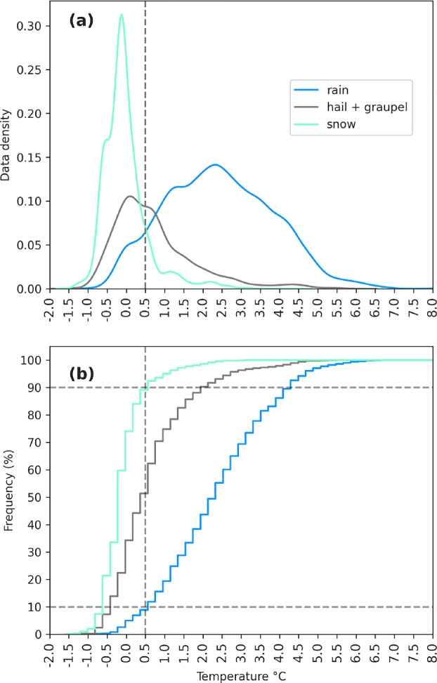
(a) Density distribution of snow (light green), hail + graupel (grey), and rain (blue) data according to temperature. The dotted line is located at 0.5 °C, below which 90% of the snow records are located and 90% of rain records are located above the same value. (b) Cumulative frequency graph expressed in percentages for snow, hail, and rainfall records according to temperature values. The horizontal dotted lines mark the location of 90% (upper line) and 10% (lower line). The vertical line marks the 0.5 °C value.
Diurnal cycle
Figure 3 allow us to examine more closely the favorable conditions for the occurrence of the three precipitation types during the day and night. In our analysis, we defined “day” as the period from 6:00 to 18:00 LST (Local Sidereal Time) and “night” as the period from 18:00 to 6:00 LST. Based exclusively on the observational data, we observe that the three precipitation types can occur at any time of the day but with some hours where the frequency is higher than others. For instance, snow is more likely to occur during the night and early morning (18-6h LST). Its highest peak takes place at 01h and then decreases until midday where an increase is observed between 13h and 15h with no occurrence noted at 16h. However, by 18h, the frequency begins to rise again. Hail and graupel also occur during the early morning, with a slight peak at midday; scarce frequency is observed between 4h and 6h LST. As the day progresses, their frequency increases, reaching a higher concentration between 11h and 14h LST and remaining stable from 17h onwards. Conversely, rain concentrates its maximum occurrence during the daytime (6h–18h LST); the closer to noon, the higher frequency of occurrence. The frequency of rain is scarce during the early morning from 2h until 5h LST.
Fig. 3.

Diurnal cycle in LST of the probability frequency for snow (light green), hail + graupel (gray), and rain (blue) calculated using observational data from 89 events from late November 2022 to March 2023.
Precipitation type fraction
By examining the distribution of precipitation types across different temperature ranges and throughout the diurnal cycle, we have determined the proportion of each precipitation type during both day and night, as depicted in Fig. 4. We have modeled these fractional values based on the observational data, demonstrating good consistency between the two (further details are provided in Section "Modelling precipitation fraction"). In a broader context, the liquid and solid phases are nearly equally distributed, with the former accounting for 51.4% and the latter for 48.6%, based on observational data. Within the solid phase, snow is slightly more predominant than hail and graupel. However, when analyzing the data separately for day and night, a distinct pattern emerges. During daylight hours, rain is the dominant form of precipitation, representing approximately 66.9%, while snow, hail, and graupel have a relatively smaller share (33.1% combined). The pattern changes significantly at night, with the solid phase gaining prominence and accounting for 77.4% of total precipitation. During this period, snow comprises 50.9% of the solid phase, while hail and graupel contribute 26.5%. The total fractional distribution, in our model, exhibits a bias of 0.75%, indicating a slight deviation from observed data. However, when this bias is separated into daytime and nighttime fractions, we find a bias of 2.61% and 7.31% respectively (see Table 3). This high bias in the night fraction is due to the more complex distribution of night temperature compared to diurnal one, since the precipitation phases depend on external factors that are outside of the limits of this study.
Fig. 4.
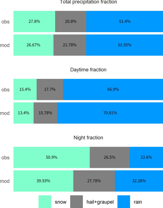
Comparison of Observed (obs) and Modeled (mod) Precipitation Type Fractions. This figure depicts the fractional contributions of different precipitation types (rain, graupel-hail, and snow) to total precipitation, during day and night. The modeled values are averaged over evenly distributed day and night periods (50–50%), based solely on temperature, while the observational values are derived from in-situ Parsivel2 disdrometer data, which accounts for actual precipitation events.
Table 3.
This is an extended data table.
| Precipitation type | Bias total (%) | Bias day (%) | Bias nigth (%) |
|---|---|---|---|
| Snow | − 1.13 | − 2.00 | − 10.97 |
| Rain | 0.15 | 3.91 | 9.68 |
| Hail+Graupel | 0.98 | − 1.92 | 1.28 |
| Absolute bias | 0.75 | 2.61 | 7.31 |
Comparison of model bias for different precipitation types in total, day, and night.
Future changes in precipitation types
Temperature thresholds and precipitation transformation
We have estimated how increases in temperature could modify the types of precipitation under the SSP2-4.5 and SSP5-8.5. Details are found in Section "Methods". The projections, as shown in Table 4 and summarized in Fig. 5, are driven by the expected increases in temperature under these scenarios.
Table 4.
Decadal Projections of Precipitation Types from 2030 to 2090 under the CMIP6 SSP2-4.5 and SSP5-8.5 scenario.
| SSP2-4.5 | SSP5-8.5 | |||||||
|---|---|---|---|---|---|---|---|---|
| Snow | Rain | H+G | Snow | Rain | H+G | |||
| 2030 | 0.6 ± 0.4 | 14.4 ± 7.2 | 65.3 ± 9.4 | 20.3 ± 2.2 | 0.7 ± 0.5 | 12.0 ± 7.3 | 68.6 ± 10.4 | 19.4 ± 3.1 |
| 2040 | 0.9 ± 0.5 | 9.4 ± 6.6 | 72.7 ± 10.4 | 17.9 ± 3.8 | 1.3 ± 0.5 | 5.3 ± 4.9 | 80.6 ± 10.0 | 14.1 ± 5.2 |
| 2050 | 1.2 ± 0.5 | 5.6 ± 5.2 | 79.7 ± 10.5 | 14.7 ± 5.2 | 1.8 ± 0.7 | 2.2 ± 3.4 | 88.9 ± 9.5 | 8.9 ± 6.1 |
| 2060 | 1.5 ± 0.6 | 3.5 ± 4.2 | 84.6 ± 10.2 | 11.8 ± 6.0 | 2.5 ± 0.9 | 0.6 ± 1.5 | 95.4 ± 6.5 | 4.0 ± 5.0 |
| 2070 | 1.7 ± 0.7 | 2.4 ± 3.9 | 87.9 ± 10.4 | 9.7 ± 6.5 | 3.1 ± 1.2 | 0.2 ± 0.7 | 98.3 ± 4.2 | 1.6 ± 3.4 |
| 2080 | 1.9 ± 0.8 | 1.7 ± 3.1 | 90.6 ± 9.5 | 7.7 ± 6.4 | 3.9 ± 1.4 | 0.0 ± 0.2 | 99.5 ± 1.8 | 0.5 ± 1.6 |
| 2090 | 2.1 ± 0.8 | 1.3 ± 2.8 | 92.1 ± 9.1 | 6.6 ± 6.3 | 4.6 ± 1.7 | 0.0 ± 0.1 | 99.8 ± 1.1 | 0.2 ± 1.0 |
The table presents averaged projections of temperature increase () in Celsius Degrees, snow fraction, rain fraction, and hail + graupel (H+G) fraction for each decade. Values are derived from CMIP6 SSP2-4.5 and SSP5-8.5 model outputs. The error margin represents the midpoint between the 10th and 90th percentile projections.
Fig. 5.
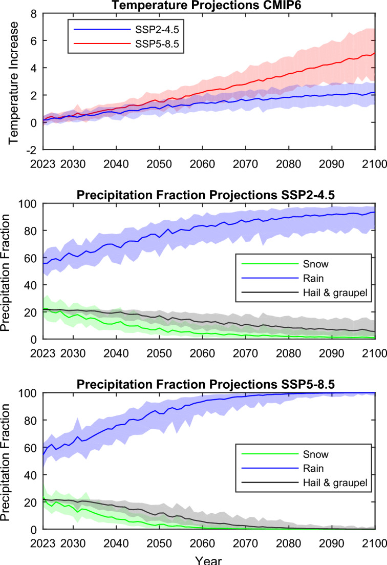
Future Projections of Precipitation Types with Error Margins and Temperature Increase () under SSP2-4.5 and SSP5-8.5 Scenarios. Top panel: CMIP6 model-based temperature increase projections under SSP2-4.5 (blue) and SSP5-8.5 (red) scenarios, with the shaded areas representing the 10th to 90th percentile range of the projections. Middle panel: Projected changes in the occurrence of three types of precipitation - snow (green), rain (blue), and hail & graupel (gray) - from 2023 to 2100 under the SSP2-4.5 scenario, including error margins. Bottom panel: Similar precipitation fraction projections under the SSP5-8.5 scenario, also including error margins.
The critical temperature points and the corresponding years in each scenario, as summarized in Table 4, offer an insightful view of the disparity in the rate of temperature increase between the two scenarios. A C increase in temperature is expected to occur by the decade of 2050 in the SSP2-4.5 scenario, whereas it is anticipated a decade earlier, by the 2040s, in the more severe SSP5-8.5 scenario.
A similar pattern is observed with a 1.5C rise, which is expected to happen in the 2060s under SSP2-4.5 but occurs 20 years earlier, by the 2040 decade, under SSP5-8.5. The disparity is even more pronounced with a 2 °C increase, which is projected to occur by the 2090 decade under SSP2-4.5 (2.1C), while it is expected by the 2060s under SSP5-8.5 ().
It is worth noting that SSP2-4.5 does not project a temperature rise beyond 2 °C within the current century. However, under the SSP5-8.5 scenario, the temperature continues to rise, reaching 3 °C by the 2070s and 4 °C by 2090s.
These results underscore the acute differential impacts of the two climate change scenarios on the transformations in precipitation types, particularly the transition from solid to liquid forms. The more drastic changes under SSP5-8.5 imply a quicker disappearance of solid precipitation types, with profound implications for regions where these forms of precipitation are predominant.
Projected alterations in precipitation types
As shown in Table 4, future projections for precipitation types under both SSP2-4.5 and SSP5-8.5 scenarios reveal significant changes in the composition of precipitation as a response to rising temperatures.
Figure 5 presents a stark picture of the alterations in precipitation types with rising temperatures throughout the decades from 2030 to 2090 for both scenarios. Our model indicates a significant shift from solid to liquid precipitation with just a 2 °C increase in temperature, transitioning from around 50% solid precipitation at present to less than 10% with the 2 °C increase. The SSP 2-4.5 scenario shows a consistent pattern of increase in average temperature. Notable changes are evident in the precipitation fractions over the decades. The snow fraction shows a decreasing trend, going from an average of 14.4% in the 2030s to only 1.3% in the 2090s. In parallel, the rain fraction exhibits a continuous increase, starting from 65.3% (± 9.4%) in 2030 and reaching 92.1% (± 2.8%) in 2090. This change suggests a transition from solid to liquid precipitation, influenced by the increase in global temperatures. Nevertheless, other factors should be considered, like the easterlies wind pattern over Central Andes Mountain26,30–33, the snow-ice albedo, clouds, water vapor and aerosols feedbacks which are linked with the elevation-dependent warming mechanisms34,35, South American Monsoon32, Amazonian convective systems36,37, and the high-altitude air temperature over the Andes forced by the tropical sea surface temperature2,20,38,39, but all that are beyond the scope of this research. On the other hand, the hail fraction also decreases, from 20.3% (± 2.2%) in the 2030s to 6.6%(± 6.3%) in the 2090s.
Regarding the precipitation fractions in the same period for the SSP 5-8.5 scenario, substantial changes are observed. The snow fraction shows a drastic decrease, starting from an average of 12.0% in the 2030s, descending to values below 1% in the 2060s (0.6 ± 1.5%) and reaching values close to zero in the following decades. In parallel, the rain fraction experiences a considerable increase, starting with 68.6% in the 2030s and reaching up to 99.8% ± 1.1% in the 2090s. In addition, the hail fraction also shows a significant decrease, from 19.4% in the 2030s to much lower values in the following decades.
Discussion
Shifts in precipitation types and its implications
Glacier retreat at Huaytapallana is linked to the temperature rise, as a temperature-induced change from snow to rain can increase glacier decline40. Our results show potential future changes in precipitation types, with an increased frequency of rain events for both SSP2-4.5 and SSP5-8.5 scenarios (Fig. 5), and a reduction in the frequency of solid events (snow, hail and graupel), which could have profound implications for glacier dynamics and downstream water resources. Thus, glacier retreat can be expected across the Huaytapallana glacier due to higher air temperatures increasing heat transfer and inducing a change from snow to rain40. These findings stress the urgency of integrating these insights into climate modeling. The data obtained in this study have the potential to improve the accuracy of regional climate models. For example, the incorporation of specific precipitation type data can improve the representation of surface processes in climate models, which, in turn, can enhance projections of changes in glacial basin hydrology4. It is important to note the limitations of this study, as the hourly local observed data cover only one year of precipitation measurements. However, no major changes or trends have been detected in the past five decades of historical observed precipitation data across the Central Andes41–43. Furthermore, the precipitation distributions found here are consistent with other observational data from the Andes and the Swiss Alps18.
Our study provides valuable insights into the changing precipitation phases in the periglacial zone of the Peruvian Andes. Glacier retreat alters land use and ecosystem service values44. These findings also underscore the importance of integrating such insights into hydrological modeling to develop better adaptation policies for the Andean region45–47. By incorporating these detailed observations into climate models, we can enhance predictive accuracy and inform policies that promote sustainable management, ultimately safeguarding glaciers and their vital ecosystem services48.
Effects of precipitation types changes on glacier mass balance
The key driver of the mass balance of Peruvian glaciers is precipitation dynamics49. This is principally because the solid/liquid precipitation is linked with albedo, which determines the magnitude of net shortwave radiation, the most important contributor to energy available for melt. This can be understood, since the increase in albedo during snowfall is empirically modeled to be proportional to the snowfall intensity by a factor of 0.02 (mm w.e.) -150.
Using a physically based Energy and Mass Balance Model49, the mass, energy, and water fluxes were simulated at the point scale of five Peruvian study sites across the Andes. The assessment revealed that a 2 °C air temperature increase resulted in a decrease in the proportion of snowfall in total precipitation, ranging from 53 to 0.8% from lower to higher Peruvian glaciers, respectively. This led to lower albedos by between 0.11 and 0.03, respectively.
Similarly, our results indicate that snowfall frequency will be reduced by about 60% and 80% with air temperature rises of about 1 °C and 2 °C, respectively, compared to current times (Fig. 6). Thus, albedo reduction is expected due to the elevation-warming dependency of the superficial snow cover and of the snow/rain ratio34. Reviewing future changes in temperature (Fig. 5), a 1 °C rise or a 60% reduction in snowfall frequency is projected to occur around 2050 and 2040 for SSP2-4.5 and SSP5-8.5 scenarios, respectively. Similarly, a 2 °C rise or an 80% reduction in snowfall frequency is expected to occur around the 2070s and 2050s for SSP2-4.5 and SSP5-8.5, respectively.
Fig. 6.

Relationship between Temperature and Precipitation Types. This figure delineates the probability of occurrence of each precipitation type (rain, graupel-hail, and snow) as a function of temperature. Note that the combined probabilities sum to 1 at any given temperature. The colored curves correspond to the parameterized fit for each precipitation type, providing a graphical representation of their likelihood at different temperatures. The derived equations of these fitted curves are presented in Section "Modelling precipitation fraction". This visualization aids in understanding the inherent relationship between temperature and the distribution of precipitation types.
On the other hand, the heat flux directly transferred from precipitation is less than 1 , with higher values occurring during the wet season49. Although precipitation over Andean glaciers carries an advected heat amount, it is very low49,50, and this is usually not considered in the surface energy and mass balance
Differential impacts of snow, graupel, and hail on glacier processes
In terms of the impact on weather and climate patterns, the rain-snow perspective has been widely assessed in different literature10,11,13,16; however, very few of them have taken into account the existence of graupel and hail within the solid phase. While snow impact in glacier dynamics has been demonstrated in the literature2,51,52, information related to hail’s impact on glacier accumulation processes remains unknown. Several factors have contributed to this limited level of understanding. For instance, hail events or hailstorms are very short in duration (some can last only a few minutes) and are difficult to model and collect direct data, especially in places with complex topography53. Both graupel and hail can have different effects due to their different fall speeds and densities. For example, hail can cause more damage on the ground due to its larger size and higher fall speed54, while graupel can contribute to the cooling of the atmosphere due to smaller stones and will be more effective in extracting heat from the environment55. Thus, the influences of graupel and hail when they reach the glacier surface, either contributing to glacier mass accumulation or promoting runoff in the presence of rainfall, remain unclear but could have important implications for glacier dynamics and downstream water resources, as demonstrated in studies by Sommers and Mark45. To address this gap in knowledge, it would be necessary to take several factors into account, such as the volume of graupel or hail, the pre-existing surface conditions of the glacier (such as temperature, albedo, and surface roughness), as well as the post-deposition weather conditions. Also, atmospheric phenomena such as wind transport, sublimation, or evaporation could alter these processes, adding an additional layer of complexity to their modeling and prediction.
The presence of graupel and hail in our study events was relevant. Firstly, because it represents nearly 43% of the solid phase in the present (Fig. 4) and secondly, the future scenarios (see Fig. 5) highlight that graupel-hail would be predominant over snow. As we transition into these future scenarios, the dominant role of graupel-hail could fundamentally shift our understanding of glacier dynamics and responses to climate change. Therefore, the study of hail impacts on glaciers represents an open and promising field of research, with potential implications for our understanding of glacier dynamics and responses to climate change.
Future projections of precipitation types
Instead of relying solely on precipitation generated by models to assess precipitation phases, it is preferable to use near-surface air temperature in the way that was done in the present research. Thus, projections of Andean precipitation types give us more detailed information. In this context, our results in Fig. 5 for SSP2-4.5 scenario suggest that more than an 80% of future rainfall occurrence will be dominant as of 2060s–2070s, with less than 5% of snowfall events (Table 4). For the case of SSP5-8.5 scenario, the aforementioned range is giving by the 2050s–2060s (Table 4). In both cases, hail and graupel occurrences will be reduced by less than the 5% around the 2090s and 2050s, for SSP2-4.5 and SSP5-8.5, respectively. Therefore, water sustainability is going to be affected for the increment of rainfall (warmer) precipitation, which will contributes to the faster retreat of glaciers. The current mountain ecosystem is intrinsically connected with solid (cold) precipitation, retaining solid water in the glaciers principally during seasonal precipitation months (October–May). This stored water is released during seasonal no-precipitation months (April–September) to supply freshwater to Andean regions2,3,6. However, statistically, both future SSP scenarios indicate that solid precipitation will begin to diminish from the mid-21st century compared to the present, initiating a new climate state characterized by predominantly liquid precipitation. This is consistent with studies such as Yang et al.17, who analyzed differences in precipitation types between the Arctic, Antarctica, and Tibet, finding that increasing temperature leads to a transition from snow to rain in all of these regions. In the tropical Andes, our research complements these findings by providing empirical data from a disdrometer, something that has not been widely reported in the literature. Comparing our projections with those from studies in other mountain regions, we observe similar patterns of change in the fraction of precipitation types, underscoring the universality of climate change impacts in high mountain areas.
The melting layer and high-altitude precipitation dynamics
In the context of our study at 4709 m ASL, where nearly 50% of the precipitation is solid, the proximity to the melting layer provides a unique opportunity to observe and analyze the transition of precipitation types. The melting layer, typically located between 4500 and 5000 m ASL in the Andes56,57, is the region where falling snow begins to melt and transition into rain. This transition zone is of particular interest for meteorological studies and climate models, as the type of precipitation (solid or liquid) can have significant impacts on surface processes, energy balance, and hydrological cycles. Valdivia58 found that the melting layer frequency peaks on 4700 m ASL in the Mantaro Valley. This is particularly relevant in the periglacial environment, where the type of precipitation can influence the thermal regime of the ground, the formation and evolution of periglacial landforms, and the dynamics of glacier melt and retreat.
Furthermore, as climate change is expected to raise the altitude of the 0 °C isotherm59–61, these observations can provide valuable insights into how shifts in the melting layer might affect precipitation patterns and glacier dynamics in the future. For instance, an increase in the proportion of liquid precipitation could accelerate glacier melt rates and impact water resources downstream. Therefore, the strategic placement of instruments near the melting layer is essential for improving our understanding of precipitation processes and their implications for glacier environments and climate change adaptation strategies.
Addressing instrumental challenges: classification of graupel and hail
Graupel and hail are both types of solid precipitation, but they form through different processes and have different characteristics. Hailstones originate within thunderstorms when updrafts transport raindrops into extremely cold sections of the storm, hailstones can grow rather large, exceeding 5 mm in diameter, and descend at remarkable speeds54. On the other hand, graupel, also known as soft hail or snow pellets, forms when supercooled water droplets freeze onto a snowflake, forming a small, soft, white pellet. Graupel is typically smaller than hail, with a maximum diameter of about 5 mm, and it falls at slower speeds55. Because of the similarities in size and fall speed between small hail and large graupel, the Parsivel2 may sometimes misclassify graupel as hail, considering that the Parsivel2 does not include the “graupel” classification. This limitation can be addressed by considering a “graupel-hail” classification. This combined classification would account for the possibility of misclassification and provide a more accurate representation of the types of solid precipitation that are occurring.
Methods
Observational data
Temperature observations recorded at 1-minute intervals were obtained from Lufft WS500-UMB compact weather station (CWS). It’s good performance working in extreme weather conditions (between − 50 °C to C) and its C accuracy make it the best option for the assessment of high mountain atmospheric conditions (further details are found in62). Past studies such as Valdivia et al.63 made an evaluation and inter-comparison with different sensors and conventional weather stations, finding an acceptable performance in the Central Andes. Both the weather station and Parsivel2 disdrometer are installed side by side at 4709 m ASL (11° 56′ 18.06″ S, 75° 4′ 9.44″ W) at Glacier and Mountain Ecosystem Monitoring Center- CEMGEM (Fig. 1). Additionally, to perform bias correction of the CMIP6 models, we utilized 10 years of hourly temperature data (2013–2023) recorded by a nearby meteorological station, SENAMHI - Huaytapallana (11° 55′ 37.81″ S, 75° 3′ 42.7″ W), 2km away from CEMGEM at 4700 m ASL. The OTT Parsivel2, a second-generation optical-laser disdrometer introduced by HydroMet, measures the size and velocity of hydrometeors23. It can detect hydrometeor sizes ranging from 0 to 25 mm, with a minimum detectable size of approximately 0.25 mm64. The device can identify drop velocities between 0.2 and 20 m/s. All this information feeds into a 32 × 32 size matrix, structuring hydrometeor diameter versus drop velocity data at one-minute intervals22. The Parsivel2 software also calculates the precipitation rate and radar reflectivity65. Additionally, the software calculates hydrometeor types, and rather than using precipitation amounts, which can present challenges in terms of data validation, we are primarily interested in the classification of precipitation types in this study. These are coded according to the World Meteorological Organization’s (WMO) table 4680. An explanation of these codes is provided in an extended data Table 1, to enhance understanding and accessibility for readers unfamiliar with this specific coding system.
The Parsivel2’s performance is reliable under non-extreme conditions, particularly in moderate rainfall and for midsize drops23,66. However, at 3300 m ASL, the Parsivel2 has been found to systematically underestimate total rainfall by around 16% for a single rainfall event57,64,67. Additionally, Parsivel2 has the limitation in measuring very small hydrometeors and irregularly shaped hailstones or complex snowflake shapes22. Therefore, the use of precipitation type frequency, rather than precipitation amount, can be a robust measure against uncertainties in the measurement of precipitation amounts and, thus, offer better insights into the formation of different precipitation types.
In this study, we have grouped hail and graupel into a single category. This decision was driven by the limitations of the Parsivel2 disdrometer, which does not distinguish “graupel” as a separate type of hydrometeor. Given the physical form similarities between hail and graupel, this grouping helps reduce classification uncertainty.
Modelling precipitation fraction
To assess the impact of climate change on precipitation types, we have developed a mathematical model to understand how precipitation patterns will alter. The Fig. 7 shows a methodology flow diagram. By integrating temperature-dependent precipitation probabilities with projected temperature distributions, we can predict the future fractions of different precipitation types, such as snow, rain, and graupel. To achieve this, we evaluate the integral:
| 1 |
where represents the projected fraction of a specific precipitation type in the future, accounting for a temperature increase . is the temperature-dependent precipitation function, which specifies the fraction or probability of a particular type of precipitation occurring at a given temperature . For example, might show that snow is more likely at lower temperatures, while rain becomes more probable at higher temperatures. represents the probability distribution of temperatures, adjusted for future changes (). It reflects the likelihood of encountering each temperature within the given range, considering climate change impacts. For instance, as temperatures increase, the distribution shifts, indicating higher probabilities for warmer temperatures. The product gives the joint probability that a specific precipitation type will occur at a particular temperature, weighted by the likelihood of that temperature in the future. Integrating this product over the entire temperature range, from to , sums these weighted probabilities to obtain the total fraction .
Fig. 7.

Methodology flow diagram for computing future precipitation types. The diagram includes temperature distribution functions for day and night temperatures, temperature projections under different climate scenarios (SSP2-4.5 and SSP5-8.5), and temperature-precipitation functions for snow, rain, and graupel. By integrating the temperature-dependent precipitation function with the adjusted temperature distribution function , we predict the future fractions of different precipitation types under the influence of climate change.
Utilizing observational data from a Parsivel2 disdrometer and compact weather stations, we fitted sigmoid functions to estimate the temperature-dependent precipitation functions (R) of snow (), rain (), and hail/graupel () as a function of temperature. We found this methodological approach suitable due to the limited data availability (one season), the need to maintain consistency with climate models and to avoid additional uncertainties in our modeling. This methodology using only air temperature has been applied in similar studies about precipitation types (e.g.14,17,18,68).
Sigmoid functions describe the transition from one type of precipitation to another as a function of temperature. For snow () and rain (), we use:
| 2 |
| 3 |
where and are the midpoints (50%) of the transition for each type of precipitation. Specifically, represents the temperature at which there is a 50% transition for snow to other types, and represents the temperature at which there is a 50% transition from other types to rain. Parameters and define the slope of these transitions, indicating the rate of change from 0 to 100% (or vice versa) for each precipitation type. The hail fraction function, , was obtained from the complement of the snow and rain fractions: . The observed and fitted curves are shown in Fig. 6.
The observed air temperature distribution function (f) is fitted using Gamma distributions. The f of temperature was estimated separately for day and night using maximum likelihood estimation. By using the BIC (Bayesian Information Criterion) and AIC (Akaike Information Criterion) criteria (see Extended data Table 5) we found that the day distribution followed a gamma distribution:
| 4 |
where is the gamma function, and and are the parameters computed by maximum likelihood estimation. The night distribution, on the other hand, followed an inverse gamma distribution:
| 5 |
where and are the parameters computed by maximum likelihood estimation. The total of temperature distribution (f) is described by the addition of day and night distribution as . The use of and to describe the total temperature distribution was necessitated by the bimodal temperature behavior observed in our study zone, characterized by distinct daytime and nighttime temperature patterns. The value of each parameter and the efficiency of each adjustment model are shown in Extended data Table 6.
Table 5.
This is an extended data table.
| Day distribution | BIC | AIC | Night distribution | BIC | AIC |
|---|---|---|---|---|---|
| Gamma | 36813.57 | 36799.17 | Inverse-Gamma | 9381.009 | 9368.298 |
| Inverse-Gaussian | 36938.43 | 36924.03 | Beta-prime | 9437.259 | 9368.298 |
| Log-normal | 36960.44 | 36946.04 | Log-normal | 9564.105 | 9551.394 |
| Beta-prime | 37152.77 | 37138.37 | Inverse-Gaussian | 9569.165 | 9556.454 |
| Weibull | 37170.97 | 37156.56 | Gamma | 9783.519 | 9770.808 |
| Inverse-Gamma | 37232.79 | 37218.39 | Weibull | 11404.152 | 11391.441 |
| Inverse-Weibull | 38830.53 | 38816.12 | Rayleigh | 16719.690 | 16713.335 |
Model comparison using BIC (Bayesian Information Criterion) and AIC (Akaike Information Criterion) methods for day and night distributions. Selected models are highlighted in bold where the less value, better the fit.
Table 6.
This is an extended data table.
| Model | Parameters | Estimated values | RSE | Log-likelihood |
|---|---|---|---|---|
| R1 (Snow) | , | 0.1381, 0.4851 | 0.0202 | |
| R2 (Rain) | , | 1.0012, − 0.6004 | 0.0288 | |
| R3 (Hail) | R1, R2 | 0.0460 | ||
| Gamma (Day) | , | 17.9876, 0.3719 | − 18397.58 | |
| InvGamma (Night) | , | 47.5039, 234.8284 | − 4682.15 |
Summary of fitting models for precipitation fractions and temperature distributions.
Under a climate change scenario, the temperature distribution shifts by an amount equal to the respective temperature increase () under the different climate scenarios (SSP2-4.5 and SSP5-8.5). We assume that the shape of the temperature distribution will remain unchanged in the future. This is a simplification, and while it is a common approach in climate studies due to the complexities and uncertainties of predicting future climate dynamics, it does introduce some level of uncertainty in our projections.
The model was validated by comparing the modeled precipitation fractions () against the observed fractions from the disdrometer data. We computed the bias as the absolute difference between the modeled and observed fractions. Extended Data Fig. 8 shows how the model predicts precipitation types changes while the temperature increases.
Fig. 8.

This is an Extended Data Figure. Model Predictions of Precipitation Type Changes in Relation to Temperature Changes (Eq. 1). This figure provides a predictive view of the shift in precipitation types in response to increasing temperatures. Starting from a baseline condition where approximately 50% of precipitation is in the solid phase, the model illustrates the dramatic reduction in solid precipitation with rising temperatures.
Extended data Table 3 provides an evaluation of the total model bias for different types of precipitation and their absolute biases. The total biases indicate the general tendency of the model in estimating the precipitations. For snow, the model slightly underestimates the quantity, with a total bias of − 1.13%. In the case of rain, the model shows a small bias towards overestimation, with a total bias of 0.15%. Regarding hail-graupel, the total bias is 0.98%, indicating a slight overestimation.
The absolute bias provides a measure of the overall magnitude of the deviations, regardless of whether they are overestimations or underestimations. In this case, the absolute bias for snow, rain, and hail plus graupel is 0.75%, 2.61%, and 7.31%, respectively. These values highlight that although the model tends to underestimate snow and overestimate rain and hail plus graupel, the degree of these deviations is relatively small.
Furthermore, a sensitivity analysis was conducted to assess the robustness of the model. This analysis included the evaluation of different PDFs for temperature, such as Weibull, Gamma, and inverse Gamma distributions (see Extended data Table 5).
This integral approach allows us to capture the contributions from all possible temperatures, providing a robust and comprehensive projection of how different precipitation types are expected to occur in the future. The methodology leverages numerical methods to solve the integral. This projection is crucial for understanding and preparing for future climate impacts on precipitation patterns.
CMIP6 data and climate change scenarios
The Coupled Model Intercomparison Project Phase 6 (CMIP6) is an international collaborative framework, initiated by the World Climate Research Program (WCRP). These scenarios provide useful projections for the scientific community and policymakers about potential future climates.
Several studies have shown that temperature variables generated by global climate models (GCM) are high accurately reproduced over Central Andes20,38,69,70
Specifically, Yarleque et al.20 processed air temperature over Quelccaya Ice Cap at southern Peru, between 5300 and 5680 m ASL, from CMIP5 GCM data set. In this study, and following Yarleque20, two scenarios from CMIP6 were used: Shared Socioeconomic Pathway (SSP) 2-4.5 and SSP5-8.5. SSPs are narratives about potential global futures, including sustainable development, inequality, fossil-fueled development, and innovation.
The SSP2-4.5 scenario reflects a continuation of historical social, economic, and technological trends, with greenhouse gas emissions stabilizing and radiative forcing reaching 4.5 W/ by 2100. The SSP5-8.5 scenario depicts a fossil fuel-reliant world with rapid economic growth and urbanization, leading to radiative forcing of 8.5 W/ by 210071.
The GCM Near-surface air temperature (tas) were selected from the CMIP6 variables since observed data used in the precipitation phase modelling is the air near-surface temperature gauged from a weather station. The list of the 40 CMIP6 models used in this research are presented in the extended data Table 7. Subsequently, each CMIP6 model time series was bias corrected20 using hourly observed data from the SENAMHI-Huaytapallana Meteorological station, located 2km away to CEMGEM but closer to Huaytapallana glacier. This station contains longer-term temperature data over the period 2013-2023. The bias correction of raw CMIP6 projections was done by subtracting the value obtained (bias) when the mean of the raw CMIP6 data and the available observations are subtracted over a reference period.
Table 7.
This is an extended data table.
| Model | Variant label | Center (Country) | Resolution |
|---|---|---|---|
| ACCESS-CM2 | r1i1p1f1 | Commonwealth Scientific and Industrial Research Organisation (Australia) | x |
| ACCESS-ESM1-5 | r1i1p1f1 | x | |
| AWI-CM-1-1-MR | r1i1p1f1 | Helmholtz Centre for Polar and Marine Research (Germany) | x |
| BCC-CSM2-MR | r1i1p1f1 | Beijing Climate Center (China) | x |
| CAMS-CSM1-0 | r1i1p1f1 | Chinese Academy of Meteorological Sciences (China) | x |
| CanESM5-CanOE | r1i1p2f1 | Canadian Centre for Climate Modelling and Analysis, Environment and Climate Change (Canada) | x |
| CanESM5 | r1i1p2f1 | x | |
| CanESM5 | r1i1p1f1 | x | |
| CESM2 | r1i1p1f2 | The National Center for Atmospheric Research (USA) | x |
| CESM2-WACCM | r1i1p1f1 | x | |
| CIESM | r1i1p1f1 | Tsinghua University (China) | x |
| CMCC-CM2-SR5 | r1i1p1f1 | Fondazione Centro Euro-Mediterraneo sui Cambiamenti Climatici (Italy) | x |
| CNRM-CM6-1 | r1i1p1f2 | Centre National de Recherches Météorologiques (France) | x |
| CNRM-CM6-1-HR | r1i1p1f2 | x | |
| CNRM-ESM2-1 | r1i1p1f2 | x | |
| EC-Earth3 | r1i1p1f1 | EC-Earth European Consortium | x |
| EC-Earth3- Veg | r1i1p1f1 | x | |
| FGOALS-f3-L | r1i1p1f1 | Chinese Academy of Sciences (China) | x |
| FGOALS-g3 | r1i1p1f1 | x | |
| FIO-ESM-2-0 | r1i1p1f1 | First Institute of Oceanography (China) | x |
| GFDL-CM4 | r1i1p1f1 | NOAA (USA) | x |
| GFDL-ESM4 | r1i1p1f1 | x | |
| GISS-E2-1-G | r1i1p1f1 | Goddard Institute for Space Studies (USA) | x |
| GISS-E2-1-G | r1i1p3f1 | x | |
| HadGEM3-GC31-LL | r1i1p1f3 | Met Office Hadley Centre (UK) | x |
| HadGEM3-GC31-MM | r1i1p1f3 | x | |
| UKESM1-0-LL | r1i1p1f2 | x | |
| INM-CM4-8 | r1i1p1f1 | Institute for Numerical Mathematics (Russia) | x |
| INM-CM5-0 | r1i1p1f1 | x | |
| IPSL-CM6A-LR | r1i1p1f1 | Institut Pierre Simon Laplace (France) | x |
| KACE-1-0-G | r1i1p1f1 | National Institute of Meteorological Sciences (Korea) | x |
| MCM-UA-1-0 | r1i1p1f2 | University of Arizona (USA) | x |
| MIROC6 | r1i1p1f1 | Japan Agency for Marine-Earth Science and Technology (Japan) | x |
| MIROC-ES2L | r1i1p1f2 | x | |
| MPI-ESP1-2-HR | r1i1p1f1 | Max Planck Institute for Meteorology (Germany) | x |
| MPI-ESM1-2-LR | r1i1p1f1 | x | |
| MRI-ESM2-0 | r1i1p1f1 | Meteorological Research Institute (Japan) | x |
| NESM3 | r1i1p1f1 | Nanjing University of Information Science and Technology (China) | x |
| NorESM2-LM | r1i1p1f1 | NorESM Climate modeling Consortium (Norway) | x |
| NorESM2-MM | r1i1p1f1 | x |
The features of the 40 CMIP6 models from which climatic data were used for this research.
Extended data
Declarations
Some journals require declarations to be submitted in a standardized format. Please check the Instructions for Authors of the journal to which you are submitting to see if you need to complete this section. If yes, your manuscript must contain the following sections under the heading ‘Declarations’:
Acknowledgements
Special thanks to PhD. Timothy Raupach for his insightful comments and suggestions of the research. His guidance was instrumental in enhancing the quality of our study. This work was done under the project ”TAMYA - Impactos de la precipitación, registrados con un radar meteorológico, en los cuerpos glaciares Andinos: Nevado Huaytapallana, CONCYTEC - 082-2021-FONDECYT”. We also want to thank: Gobierno Regional de Junín and Oficina Desconcentrada de la Región Centro de Lima - INAIGEM. We recognize the efforts of the World Climate Research Programme, which facilitated and advanced CMIP6 through its Working Group on Coupled Modelling. We are grateful to the climate modeling groups for their production and provision of model output, the Earth System Grid Federation (ESGF) for storing the data and enabling access, and the various funding agencies that back both CMIP6 and ESGF.”Part of the work of author Christian Yarleque was supported by the Pontificia Universidad Católica del Perú (PUCP) through the postdoctoral project ‘Projections of the Impacts of Glacial Retreat on High Andean Agriculture’ (Proyecciones de los Impactos del Retroceso Glaciar sobre la Agricultura Altoandina). This project was one of the winners of the PUCP Postdoctoral Stays 2023 (Estancias Postdoctorales PUCP 2023).” We acknowledge OpenAI’s ChatGPT, an artificial intelligence language model that significantly improved the text’s quality and clarity. The AI assisted in structuring our language and arguments. However, the final interpretations and conclusions presented in this manuscript are the responsibility of the authors. We thank Joan Ramírez Romero for providing us with a high-quality image of the glacier, which has contributed to the visual representation of our study area and Steven Wegner for the english improvement.
Author contributions
V.L., J.V., C.Y., and S.C. conceptualized the study. V.L., D.G., and R.A.L. curated the data. V.L., J.V., E.V.P., and C.Y. conducted the formal analysis and developed the methodology. V.L. and J.V. developed the software and visualized the results. V.L., J.V., and C.Y. prepared the original draft of the manuscript. V.L., J.V., E.V.P. and C.Y. reviewed and edited the manuscript. J.V., D.G., and R.A.L. validated the results. C.Y. and S.C. secured the funding and administered the project. C.Y., S.C., D.G. and R.A.L. provided the resources. C.Y. and S.C. supervised the project.
Funding
This work was done under the project “TAMYA - Impactos de la precipitación, registrados con un radar meteorológico, en los cuerpos glaciares Andinos: Nevado Huaytapallana, CONCYTEC - 082-2021-FONDECYT”.
Data Availability
Data used in this article can be provided with a previous request via e-mail to ralvarado@inaigem.gob.pe.
Code availability
The corresponding authors can provide the computer code or algorithm used to generate the results presented in the paper, which are crucial to the main claims, upon reasonable request.
Competing interests
The authors declare no competing interests.
Footnotes
Publisher's note
Springer Nature remains neutral with regard to jurisdictional claims in published maps and institutional affiliations.
These authors contributed equally: Valeria Llactayo, Jairo Valdivia and Christian Yarleque.
References
- 1.Harpold, A. A. et al. Rain or snow: hydrologic processes, observations, prediction, and research needs. Hydrol. Earth Syst. Sci.21, 1–22 (2017). [Google Scholar]
- 2.Vuille, M. et al. Rapid decline of snow and ice in the tropical Andes - impacts, uncertainties and challenges ahead. Earth Sci. Rev.176, 195–213. 10.1016/j.earscirev.2017.09.019 (2018). [Google Scholar]
- 3.Buytaert, W. et al. Glacial melt content of water use in the tropical Andes. Environ. Res. Lett.12, 114014. 10.1088/1748-9326/aa926c (2017). [Google Scholar]
- 4.Viviroli, D. et al. Climate change and mountain water resources: Overview and recommendations for research, management and policy. Hydrol. Earth Syst. Sci.15, 471–504 (2011). [Google Scholar]
- 5.Veettil, B. K. & Kamp, U. Global disappearance of tropical mountain glaciers: Observations, causes, and challenges. Geosciences9, 196 (2019). [Google Scholar]
- 6.Rabatel, A. et al. Current state of glaciers in the tropical Andes: A multi-century perspective on glacier evolution and climate change. Cryosphere7, 81–102 (2013). [Google Scholar]
- 7.Box, J. E. et al. Greenland ice sheet albedo feedback: Thermodynamics and atmospheric drivers. Cryosphere6, 821–839 (2012). [Google Scholar]
- 8.Mankin, J. S., Viviroli, D., Singh, D., Hoekstra, A. Y. & Diffenbaugh, N. S. The potential for snow to supply human water demand in the present and future. Environ. Res. Lett.10, 114016. 10.1088/1748-9326/10/11/114016 (2015). [Google Scholar]
- 9.López-Moreno, J. I. et al. Changes in the frequency of global high mountain rain-on-snow events due to climate warming. Environ. Res. Lett.16, 094021 (2021). [Google Scholar]
- 10.Kienzle, S. A new temperature based method to separate rain and snow. Wiley InterScience. www.interscience.wiley.com (2008).
- 11.Dai, A. Temperature and pressure dependence of the rain-snow phase transition over land and ocean. Geophys. Res. Lett.35, 1–7 (2008). [Google Scholar]
- 12.Ye, H., Cohen, J. & Rawlins, M. Discrimination of solid from liquid precipitation over Northern Eurasia using surface atmospheric conditions. J. Hydrometeorol.14, 1345–1355 (2013). [Google Scholar]
- 13.Ding, B. et al. The dependence of precipitation types on surface elevation and meteorological conditions and its parameterization. J. Hydrol.513, 154–163. 10.1016/j.jhydrol.2014.03.038 (2014). [Google Scholar]
- 14.Sun, F. et al. Incorporating relative humidity improves the accuracy of precipitation phase discrimination in High Mountain Asia. Atmos. Res.271, 106094. 10.1016/j.atmosres.2022.106094 (2022). [Google Scholar]
- 15.Marks, D., Winstral, A., Reba, M., Pomeroy, J. & Kumar, M. An evaluation of methods for determining during-storm precipitation phase and the rain/snow transition elevation at the surface in a mountain basin. Adv. Water Resour.55, 98–110. 10.1016/j.advwatres.2012.11.012 (2013). [Google Scholar]
- 16.Jennings, K. S., Winchell, T. S., Livneh, B. & Molotch, N. P. Spatial variation of the rain-snow temperature threshold across the Northern Hemisphere. Nat. Commun.9, 1–9. 10.1038/s41467-018-03629-7 (2018). [DOI] [PMC free article] [PubMed] [Google Scholar]
- 17.Yang, D. et al. On the differences in precipitation type between the arctic, Antarctica and Tibetan Plateau. Front. Earth Sci.9, 1–11 (2021). [Google Scholar]
- 18.L’hôte, Y., Chevallier, P., Coudrain, A., Lejeune, Y. & Etchevers, P. Relationship between precipitation phase and air temperature: comparison between the Bolivian Andes and the swiss alps/relation entre phase de précipitation et température de l’air: comparaison entre les Andes Boliviennes et les Alpes Suisses. Hydrol. Sci. J.[SPACE]10.1623/hysj.2005.50.6.989 (2005). [Google Scholar]
- 19.Liu, J. & Chen, R. Discriminating types of precipitation in Qilian Mountains, Tibetan Plateau. J. Hydrol. Reg. Stud.5, 20–32. 10.1016/j.ejrh.2015.11.013 (2016). [Google Scholar]
- 20.Yarleque, C. et al. Projections of the future disappearance of the Quelccaya ice cap in the central Andes. Sci. Rep.8, 1–11. 10.1038/s41598-018-33698-z (2018). [DOI] [PMC free article] [PubMed] [Google Scholar]
- 21.Liu, X., He, B., Zhao, S., Hu, S. & Liu, L. Comparative measurement of rainfall with a precipitation micro-physical characteristics sensor, a 2D video disdrometer, an OTT PARSIVEL disdrometer, and a rain gauge. Atmos. Res.229, 100–114 (2019). [Google Scholar]
- 22.Battaglia, A., Rustemeier, E., Tokay, A., Blahak, U. & Simmer, C. PARSIVEL snow observations: A critical assessment. J. Atmos. Oceanic Tech.27, 333–344 (2010). [Google Scholar]
- 23.Tokay, A., Wolff, D. B. & Petersen, W. A. Evaluation of the new version of the laser-optical disdrometer, OTT Parsivel. J. Atmos. Oceanic Tech.31, 1276–1288 (2014). [Google Scholar]
- 24.Flores-Rojas, J. L. et al. On the dynamic mechanisms of intense rainfall events in the central Andes of Peru, Mantaro valley. Atmos. Res.248, 105188. 10.1016/j.atmosres.2020.105188 (2021). [Google Scholar]
- 25.Giráldez, L., Silva, Y., Zubieta, R. & Sulca, J. Change of the rainfall seasonality over central Peruvian Andes: Onset, end, duration and its relationship with large-scale atmospheric circulation. Climate8, 23 (2020). [Google Scholar]
- 26.Garreaud, R. D. The Andes climate and weather. Adv. Geosci.22, 3–11 (2009). [Google Scholar]
- 27.Villalobos-Puma, E., Martinez-Castro, D., Flores-Rojas, J. L., Saavedra-Huanca, M. & Silva-Vidal, Y. Diurnal cycle of raindrops size distribution in a valley of the Peruvian central Andes. Atmosphere11, 38 (2020). [Google Scholar]
- 28.Junquas, C. et al. Understanding the influence of orography on the precipitation diurnal cycle and the associated atmospheric processes in the central Andes. Clim. Dyn.50, 3995–4017 (2018). [Google Scholar]
- 29.WMO. Manual on Codes (World Meteorological Organization, 2019).
- 30.Neukom, R. et al. Facing unprecedented drying of the central Andes? Precipitation variability over the period ad 1000–2100. Environ. Res. Lett.10, 084017 (2015). [Google Scholar]
- 31.Garreaud, R. Multiscale analysis of the summertime precipitation over the central Andes. Mon. Weather Rev.127, 901–921 (1999). [Google Scholar]
- 32.Garreaud, R., Garreaud, M. & Clement, A. The climate of the altiplano: Observed current conditions and mechanisms of past changes. Palaeogeogr. Palaeoclimatol. Palaeoecol.194, 5–22 (2003). [Google Scholar]
- 33.Minvielle, M. & Garreaud, R. D. Projecting rainfall changes over the south American altiplano. Am. Meteorol. Soc.24, 4577–4583 (2011). [Google Scholar]
- 34.Pepin, N. et al. Elevation-dependent warming in mountain regions of the world. Nat. Clim. Chang.5, 424–430 (2015). [Google Scholar]
- 35.Rangwala, I. & Miller, J. Climate change in mountains: A review of elevation-dependent warming and its possible causes. Clim. Chang.114, 527–547 (2012). [Google Scholar]
- 36.Yarleque, C. Climate of the cordillera Blanca. In Geoenvironmental Changes in the Cordillera Blanca, Peru. Geoenvironmental Disaster Reduction (eds Vilímek, V., Mark, B., Emmer, A.) 41–59 (Springer, Cham, 2024). 10.1007/978-3-031-58245-5_3. [Google Scholar]
- 37.Perry, L. B. et al. Characteristics of precipitating storms in glacierized tropical Andean cordilleras of Peru and Bolivia. Ann. Am. Assoc. Geogr.107, 309–322 (2017). [Google Scholar]
- 38.Bradley, R. S., Keimig, F. T., Diaz, H. F. & Hardy, D. R. Recent changes in freezing level heights in the tropics with implications for the deglacierization of high mountain regions. Geophys. Res. Lett.[SPACE]10.1029/2009GL037712C (2009). [Google Scholar]
- 39.Diaz, H. F. & Graham, N. E. Recent changes in tropical freezing heights and the role of sea surface temperature. Nature383, 152–155 (1996). [Google Scholar]
- 40.López-Moreno, J. I. et al. Recent glacier retreat and climate trends in cordillera Huaytapallana, Peru. Glob. Planet Chang.112, 1–11 (2014). [Google Scholar]
- 41.Lavado Casimiro, W. S., Labat, D., Ronchail, J., Espinoza, J. C. & Guyot, J. L. Trends in rainfall and temperature in the Peruvian amazon-Andes basin over the last 40 years (1965–2007). Hydrol. Process.27, 2944–2957 (2013). [Google Scholar]
- 42.Heidinger, H., Carvalho, L., Jones, C., Posadas, A. & Quiroz, R. A new assessment in total and extreme rainfall trends over central and southern Peruvian Andes during 1965–2010. Int. J. Climatol.38, e998–e1015 (2018). [Google Scholar]
- 43.Seiler, C., Hutjes, R. W. & Kabat, P. Climate variability and trends in Bolivia. J. Appl. Meteorol. Climatol.52, 130–146 (2013). [Google Scholar]
- 44.Madrigal-Martínez, S., Puga-Calderón, R. J., Bustinza Urviola, V. & Vilca Gomez, O. Spatiotemporal changes in land use and ecosystem service values under the influence of glacier retreat in a high-Andean environment. Front. Environ. Sci.10, 941887 (2022). [Google Scholar]
- 45.Somers, L. D. et al. Groundwater buffers decreasing glacier melt in an Andean watershed - but not forever. Geophys. Res. Lett.46, 13016–13026 (2019). [Google Scholar]
- 46.Baraer, M. et al. Glacier recession and water resources in Peru’s Cordillera Blanca. J. Glaciol.58, 134–150 (2012). [Google Scholar]
- 47.Mark, B. G. et al. Glacier loss and hydro-social risks in the Peruvian Andes. Glob. Planet Chang.159, 61–76 (2017). [Google Scholar]
- 48.Zhang, Z., Liu, L., He, X., Li, Z. & Wang, P. Evaluation on glaciers ecological services value in the Tianshan mountains, northwest China. J. Geog. Sci.29, 101–114 (2019). [Google Scholar]
- 49.Fyffe, C. L. et al. The energy and mass balance of Peruvian glaciers. J. Geophys. Res. Atmos.126, e2021JD034911 (2021). [Google Scholar]
- 50.Sicart, J. E., Hock, R., Ribstein, P., Litt, M. & Ramirez, E. Analysis of seasonal variations in mass balance and meltwater discharge of the tropical Zongo glacier by application of a distributed energy balance model. J. Geophys. Atmos.[SPACE]10.1029/2010JD015105 (2011). [Google Scholar]
- 51.Gurgiser, W., Marzeion, B., Nicholson, L., Ortner, M. & Kaser, G. Modeling energy and mass balance of Shallap Glacier, Peru. Cryosphere7, 1787–1802 (2013). [Google Scholar]
- 52.Taylor, L. S. et al. Multi-decadal glacier area and mass balance change in the southern Peruvian Andes. Front. Earth Sci.10, 1–14 (2022).35300381 [Google Scholar]
- 53.Raupach, T. H. et al. The effects of climate change on hailstorms. Nat. Rev. Earth Environ.2, 213–226. 10.1038/s43017-020-00133-9 (2021). [Google Scholar]
- 54.Allen, J. T. et al. Understanding hail in the earth system. Rev. Geophys.58, 1–49 (2020). [Google Scholar]
- 55.Pruppacher, H. & Klett, J. Microphysics of Clouds and Precipitation Vol. 18 of Atmospheric and Oceanographic Sciences Library. (Springer, 2010). http://link.springer.com/10.1007/978-0-306-48100-0.
- 56.Chavez, S. P., Silva, Y. & Barros, A. P. High-elevation monsoon precipitation processes in the central Andes of Peru. J. Geophys. Res. Atmos.125, e2020JD032947 (2020). [Google Scholar]
- 57.Kumar, S. et al. Rainfall characteristics in the Mantaro basin over tropical Andes from a vertically pointed profile rain radar and in-situ field campaign. Atmosphere11, 248 (2020). [Google Scholar]
- 58.Valdivia, J. M. et al. The GPM-DPR blind zone effect on satellite-based radar estimation of precipitation over the Andes from a ground based Ka-band profiler perspective. J. Appl. Meteorol. Climatol.61(4), 441–456 (2022). [Google Scholar]
- 59.Dessens, J., Berthet, C. & Sanchez, J. L. Change in hailstone size distributions with an increase in the melting level height. Atmos. Res.158, 245–253 (2015). [Google Scholar]
- 60.Xie, B., Zhang, Q. & Wang, Y. Trends in hail in China during 1960–2005. Geophys. Res. Lett.[SPACE]10.1029/2008GL034067 (2008). [Google Scholar]
- 61.Prein, A. F. & Heymsfield, A. J. Increased melting level height impacts surface precipitation phase and intensity. Nat. Clim. Chang.10(8), 771–776 (2020). [Google Scholar]
- 62.KGSTOCKGEARS. Technical Data Technical Data. Pnas1, 38–40 (2007). https://www.kggear.co.jp/en/wp-content/themes/bizvektor-global-edition/pdf/TechnicalData_KGSTOCKGEARS.pdf#view=Fit.
- 63.Valdivia, J. M. et al. Field campaign evaluation of sensors Lufft GMX500 and MaxiMet WS100 in Peruvian Central Andes. Sensors22, 1–21 (2022). [DOI] [PMC free article] [PubMed] [Google Scholar]
- 64.Valdivia, J. M., Scipión, D. E., Milla, M. & Silva, Y. Multi-instrument rainfall-rate estimation in the Peruvian central Andes. J. Atmos. Oceanic Tech.37, 1811–1826 (2020). [Google Scholar]
- 65.Valdivia, J. M. et al. Dataset on raindrop size distribution, raindrop fall velocity and precipitation data measured by disdrometers and rain gauges over Peruvian central Andes (12.0°S). Data Brief29, 105215 (2020). [DOI] [PMC free article] [PubMed] [Google Scholar]
- 66.Park, S. G., Kim, H. L., Ham, Y. W. & Jung, S. H. Comparative evaluation of the OTT PARSIVEL2using a collocated two-dimensional video disdrometer. J. Atmos. Oceanic Tech.34, 2059–2082 (2017). [Google Scholar]
- 67.Del Castillo-Velarde, C. et al. Evaluation of GPM dual-frequency precipitation radar algorithms to estimate drop size distribution parameters, using ground-based measurement over the Central Andes of Peru. Earth Syst. Environ.[SPACE]10.1007/s41748-021-00242-5 (2021). [Google Scholar]
- 68.Han, W., Xiao, C., Dou, T. & Ding, M. Arctic has been going through a transition from solid precipitation to liquid precipitation in spring. Chinese Sci. Bull63, 1154–1162 (2018). [Google Scholar]
- 69.Russell, A. M., Gnanadesikan, A. & Zaitchik, B. Are the central Andes mountains a warming hot spot?. J. Clim.30, 3589–3608 (2017). [Google Scholar]
- 70.Hofer, M., Marzeion, B. & Mölg, T. Comparing the skill of different Reanalyses and their ensembles as predictors for daily air temperature on a glaciated mountain (Peru). Clim. Dyn.39, 1969–1980 (2012). [DOI] [PMC free article] [PubMed] [Google Scholar]
- 71.IPCC. Climate Change 2021: The Physical Science Basis. Contribution of Working Group I to the Sixth Assessment Report of the Intergovernmental Panel on Climate Change (eds Masson-Delmotte, V., P. Zhai, A. Pirani, S. L. Connors, C. Péan, S. Berger, N. Caud, Y. Chen) (Cambridge University Press, 2021) 3949. https://www.ipcc.ch/report/ar6/wg1/downloads/report/IPCC_AR6_WGI_Full_Report.pdf.
Associated Data
This section collects any data citations, data availability statements, or supplementary materials included in this article.
Data Availability Statement
Data used in this article can be provided with a previous request via e-mail to ralvarado@inaigem.gob.pe.