

Abstract
Fatigue curves quantify fish swimming performance, providing information about the time () fish can swim against a steady flow velocity (Uf) before fatiguing. Such curves represent a key tool for many applications in ecological engineering, especially for fish pass design and management. Despite years of research, though, our current ability to model fatigue curves still lacks theoretical foundations and relies primarily on fitting empirical data, as obtained from time-consuming and costly experiments. In the present article, we address this shortcoming by proposing a theoretical analysis that builds upon concepts of fish hydrodynamics to derive scaling laws linking statistical properties of to velocities Uf, pertaining to the so-called burst range. Theoretical arguments, in the present study, suggest that the proposed scaling laws may hold true for all fish species and sizes. A new experimental database obtained from over 800 trials and five small-sized Cypriniformes support theoretical predictions satisfactorily and calls for further experiments on more fish species and sizes to confirm their general validity.
Keywords: fish locomotion, swimming performance, burst swimming, fatigue curve, scaling, time-to-fatigue
1. Introduction
Fish swimming performance has drawn a lot of interest in recent decades owing to its importance for fish migration, habitat selection and predator–prey interactions [1–6]. From an applied perspective, fish swimming performance estimates are used extensively in the design of fishways allowing for the passage of fish through dams, weirs, culverts and other anthropogenic barriers [7–9]. Other important applications include the design of sustainable fishing methods [10] and the optimization of practices in the aquaculture industry [11].
Two well-established experimental protocols are commonly used to characterize fish swimming performance: critical velocity and fixed velocity tests [12–14]. Both tests are typically conducted in either a swim chamber or an open channel flume, where fish swim until fatiguing. Fatigue is typically defined as the state of exhaustion where the fish rests at the downstream end of the test section and is not able to swim despite external motivation [15–17]. In the critical velocity test, a fish is forced to swim against a flow velocity Uf, which is progressively increased at fixed time intervals Δt, until the fish fatigues. The velocity and time at which fatigue occurs are then used to compute the critical velocity Ucrit [13,18,19]. Fixed velocity tests, on the other hand, consist of repeated swimming trials under a range of fixed velocities. Each trial results in a time-to-fatigue Tf—the time a fish can resist swimming against the defined steady flow velocity (Uf). By repeating trials for different values of Uf, a scatter plot of Tf (dependent variable) versus Uf (independent variable) can be produced. A predetermined model is then fitted to the data to obtain a fatigue or endurance curve [20]. Fixed velocity tests are more informative than critical velocity tests as they allow for the assessment of fish endurance over a range of flow velocities and associated swimming activity levels [21]. Three of such levels are believed to exist and hereafter are referred to as: sustained, prolonged and burst swimming [12,14,22]. Sustained swimming occurs at velocities whereby fish use primarily red muscles and aerobic processes. Utilizing somatic energy reserves, fish can theoretically maintain sustained swimming indefinitely [12,23]. Prolonged swimming is driven by both red and white muscles, and hence by both aerobic and anaerobic processes. In burst swimming, fish use primarily white muscles and anaerobic processes. Both prolonged and burst swimming are limited by anaerobic energy reserves and therefore subject to exhaustion. By convention, it is assumed that fish can endure prolonged swimming for up to 200 min, while burst swimming is usually associated with 20 s [9,12]. Actual thresholds between burst and prolonged swimming, however, are known to vary with species, size and even amongst similar individuals, so much so burst swimming has been often associated with of the order of 1 min or more in the literature [21,24,25].
Our current ability to model fatigue curves is primarily based on empirical mathematical relations between Tf and Uf, which sometimes are supported by dimensional analysis [3,20,21]. Burst and prolonged swimming are commonly associated with fatigue curves following either a log-linear or a power law [3,13,21,23–27]. A theoretical argument in support of either of these laws, however, has never been provided. In their review paper, Katopodis and Gervais [3] collected and analysed a large dataset of fatigue curves, and used a power law model to elucidate relations between Tf and Uf classified by grouping different fish species displaying a similar morphology or swimming kinematics. Nevertheless, the conceptual framework underpinning such relations remains undefined and rooted mostly on empirical grounds. Furthermore, the assessment of Katopodis and Gervais [3] highlighted that a majority of the published fatigue-curve data is limited to prolonged activity. Instead, comparatively little efforts have been made to characterize burst swimming activity [27], despite white muscles constituting the bulk of fish musculature, and burst swimming being key to dictate predator–prey interactions and to overcome velocity barriers [23,28–30], the latter directly relating to the design of fish passage systems [4,9,31].
Swimming performance, as estimated in fixed velocity experiments, is characterized by an enormous and unexplored variability where fish species, size and water temperature are often pointed out as key drivers [23,32–36]. Life-stage, sex, experience, health status and nutrition have also been seen to cause variation in fish swimming performance [37–42]. A large variability has also been reported for conspecifics of the same size in response to different fitness and/or motivation [11,35,43]. Therefore, considering a fixed velocity experiment where many fish of the same size and species are tested over a range of flow velocities at constant water temperature, it is reasonable to expect that experimental data will qualitatively spread around mean values of (figure 1). For each tested velocity, Tf will display a variability that can be described by a probability function . Typically, a fatigue curve is obtained by fitting the entire cloud of experimental data with a predetermined mathematical law (red line in the figure). This, however, only provides information about the general trend of the data but does not provide any clue about and how it varies with Uf.
Figure 1.
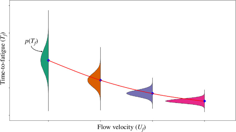
Illustration of the relationship between fish time-to-fatigue and flow velocity . For each test flow velocity value, is the probability density function of related time-to-fatigue. Blue diamonds mark the mean time-to-fatigues at a given test flow velocity. Red curve is the best-fitted line to the entire cloud of data points, referred to as fatigue or endurance curve.
The aim of this article is to present and validate a theoretical framework allowing for the statistical description of Tf versus Uf data in burst swimming. Towards this end, the following objectives are set:
to present a theoretical framework based on simple concepts of fish hydrodynamics that can statistically describe the relation between Tf and Uf, showing that (where is the mean value of Tf) and central moments of (which indeed help defining ) vary with Uf following power laws with well constrained and, in principle, universal exponents; and
to test theoretical predictions in a series of fixed velocity tests using five small-sized Cypriniformes.
2. Theoretical framework
In what follows, §2.1 reviews (and refines) the available formulations for fish drag proposed in the literature, while §2.2 draws from §2.1 to derive the sought scaling relations using energetic principles.
2.1. Fish drag
The drag force experienced by a fish while swimming can be parameterized as [23]
| (2.1) |
where is the average drag force, the symbol ‘∼’ stands for scales as, is the density of water, CD is fish drag coefficient, is total fish length (electronic supplementary material, appendix A, figure A1), is fish body depth, is the relative fish–water velocity, assumed to be identical to the flow velocity in performance tests [21,44]. The estimation of CD for swimming fish has been a matter of debate for a long time and no shared consensus has been reached [22,45–49]. At high Reynolds numbers (, where is the kinematic viscosity of water), which are typical for fish swimming at burst velocities, pressure drag is believed to dominate over friction drag [50,51] so that CD can be considered as a constant and FD is estimated as
| (2.2) |
where is a function that is herein introduced to lump the effects of parameters pertaining to fish size (i.e. L and S) and fluid properties (i.e. ).
The above formulation is, however, questionable as it completely ignores skin friction effects (and hence the dependence of CD on ReL), which some researchers argue to be significant, even at high Reynolds numbers [45,52]. While we do not intend to contribute to the debate about the nature of drag in swimming fish, in electronic supplementary material, appendix A, we demonstrate that even when skin friction effects are accounted for and considered the main source of drag, can be generally parameterized as
| (2.3) |
where ( and are defined in electronic supplementary material, appendix A) depend on water properties ( and ) and fish size, shape and tail beat amplitude (i.e. S, L and A), and the scaling exponent remains well constrained between 1.73 and 2.0. This range of also accounts for combined effects of skin friction and body undulations on CD.
2.2. Energetic considerations and scaling laws
The power (energy per unit time) expended by a fish while swimming can be estimated as . Therefore, the total energy spent by an ith fish (Ei) during a fixed velocity test can be obtained by integrating power (P) over time, between zero (i.e. the beginning of the test) and the measured time-to-fatigue (Tfi) as
| (2.4) |
When swimming is dominated by anaerobic processes, as in burst swimming, fatigue occurs when white-fibre muscles burn the available anaerobic reserves down to a critical limit which can be related to (through a conversion factor similar to an efficiency coefficient) [12,14,23] and assumed independent of . Such a critical limit clearly varies extensively among individuals [35,53,54] and cannot be predicted from first principles but it can be described statistically. Towards this end, firstly it should be noted that considering a population of fish of the same species and size and swimming at a constant water temperature, in equation (2.4), depends only on fish size, shape and tail beat amplitude (L, S and A) and water properties ( and ), and hence can be considered constant. Secondly, if averaging is taken over a representative sample of the chosen fish population, the resulting mean energy (overbar indicates averaging), can be also considered as constant. Therefore, averaging both sides of equation (2.4) leads to constant, which in turn means that scales as
| (2.5) |
Using analogous arguments as above, it is possible to derive the scaling of central moments of any order as follows.
First, considering the ith fish
| (2.6) |
Hence, defining and , equation (2.6) is rewritten as
| (2.7) |
By elevating both sides of equation (2.7) to a power k and then applying the averaging operator, equation (2.7) transforms into
| (2.8) |
As per , also can be considered a statistical trait of a fish population that is constant (and therefore independent of ), hence
| (2.9) |
Equation (2.9) provides the scaling for central moments , as sought.
3. Material and methods
The study was performed with permission from the Protection of Flora and Fauna Department of the Metropolitan City of Turin (authorization D.D. no. 4457 of 29 October 2020) and the Fauna and Ichthyofauna Technical Office of the Alessandria Province (authorization no. 1570 of 19 January 2023), under the provisions of art. 2 of the national Decree no. 26/2014 (implementation of Dir. 2010/63/EU).
3.1. Fish
Experiments were conducted on five freshwater fish species (table 1): Italian riffle dace (Telestes muticellus), common minnow (Phoxinus phoxinus), European bitterling (Rhodeus amarus), North Italian roach (Leucos aula) and common bleak (Alburnus alborella). These small-sized riverine Cypriniformes were selected because they are all common within their geographic range [55], are classified as least concerned in the IUCN red lists [56], and were expected to display interspecific variation in swimming abilities. Mean fish length ranged between 4.87 and 6.04 cm, with a standard deviation (s.d.) no larger than 0.70 cm for the five fish species (table 1). Telestes muticellus and P. phoxinus were tested in May–June 2022 and were captured from the Noce stream near Pinerolo, Italy (44°56′17.9″ N 7°23′09.1″ E) on 20 May 2022 and 11 June 2022, respectively, using electrofishing. Fish were transferred to the hatchery facility located in Porte di Pinerolo and were housed in two spring-fed flow-through holding tanks divided into six compartments. Rhodeus amarus, L. aula and A. alborella were tested in January–February 2023. They were captured from the Orba stream in the Province of Alessandria, Italy (44°45′46.7″ N 8°40′15.6″ E) using electrofishing. Rhodeus amarus were electrofished on 17 January 2023, whereas L. aula and A. alborella were caught on 30 January 2023. These fish were brought to the Alessandria Province hatchery in Predosa, Italy and were kept in spring-fed flow-through holding tanks. All fish were allowed to habituate to hatchery conditions for 3–7 days before the experimental trials.
Table 1.
Summary of experimental data reporting scientific names of the five tested Cypriniformes fish species, the total number of test fish, the number of successful fish trials n, test flow velocity Uf values, fish fork length Lf, test water temperature T and wet fish mass m.
| min | max | mean ± s.d. | ||||||
|---|---|---|---|---|---|---|---|---|
| scientific names | total test fish | successful trials (n) | tested values of Uf (cm s−1) | Lf (cm) | Lf (cm) | Lf (cm) | T (°C) | m (g) |
| Telestes muticellus | 202 | 180 | 40, 45, 50, 55 | 4 | 6.6 | 4.87 ± 0.46 | 13.4 ± 0.23 | 1.56 ± 0.49 |
| Phoxinus phoxinus | 225 | 162 | 50, 55, 60 | 3.7 | 6.8 | 4.90 ± 0.70 | 16.2 ± 0.31 | 2.05 ± 0.95 |
| Rhodeus amarus | 148 | 90 | 45, 50, 55 | 5.4 | 6.7 | 6.04 ± 0.34 | 11.7 ± 0.34 | 3.13 ± 0.59 |
| Leucos aula | 160 | 112 | 45, 50, 55 | 4.6 | 6 | 5.24 ± 0.36 | 12.7 ± 0.35 | 1.85 ± 0.45 |
| Alburnus alborella | 115 | 82 | 45, 50, 55 | 4.5 | 6 | 5.04 ± 0.38 | 11.4 ± 0.67 | 1.16 ± 0.31 |
A HOBO MX-2022 logger was used to record temperature in the holding tanks at 10 min intervals. Temperatures were 13.3 ± 0.4°C (mean ± s.d.) in 2022 and 12.3 ± 0.7°C for the experiments in 2023. All fish were fed commercial aquaria fish pellets (Tetra TabiMin) and were starved at least 24 h before testing to ensure a post-absorptive state [40,57]. Throughout the experiments, fish appeared to be in good health.
3.2. Experimental protocol
Experiments were conducted in an open channel recirculating flume with a width of 30 cm and a fixed water depth at any given test flow velocity. The water depth was slightly different for different velocities and ranged from 7 to 9 cm. The swimming arena (flume length) was 60 cm in 2022 and 80 cm in 2023, and delimited by a flow straightener in the upstream direction and a fine-meshed grid in the downstream direction. In a previous study, we demonstrated that such small differences in the length of the swimming arena had no appreciable effect on time-to-fatigue for fish swimming in burst activity level [15]. Trials were recorded from underneath and from the side of the flume using two Sony AX43 handycams with a resolution of 1920 × 1080 pixels at 50 frames per second. A pump allowed water recirculation and the flow rate was manually adjusted using the inverter (DGFIT MT 12) installed with the pump. The flow rate was measured using an AquaTransTM AT600 flow meter sensor. During trials, water temperature in the system was maintained within a narrow range of 1°C using a chiller unit (TECO TK–2000). The difference between the water temperature in the flume and the holding tanks was kept at less than 1°C to avoid any confounding effects of temperature change on swimming performance [58,59].
All fish were tested individually using a fixed velocity testing protocol. Preliminary tests were conducted on each species to determine which flow velocities could be related to burst swimming [24]. Such tests indicated that flow velocities greater than either 55 cm s−1 (European bitterling, common bleak, North Italian roach and Italian riffle dace) or 60 cm s−1 (common minnow) resulted in fish simply being unable to swim, hence leading to a large number of unsuccessful trials (a trial where Tf data is not available). Moreover, it was observed that velocities lower than 40 cm s−1 (Italian riffle dace), 45 cm s−1 (European bitterling, common bleak, North Italian roach) and 50 cm s−1 (common minnow) resulted in average times-to-fatigue significantly exceeding the commonly accepted threshold, in burst swimming, of 20 s. Therefore, fish were tested over a limited range of flow velocities. Telestes muticellus were tested at four flow velocities Uf = 40, 45, 50 and 55 cm s−1. Phoxinus phoxinus were tested at three Uf = 50, 55 and 60 cm s−1. The remaining three species, R. amarus, L. aula and A. alborella, were tested at Uf = 45, 50 and 55 cm s−1. A single fish was tested per trial at a fixed flow velocity, and no fish was tested more than once. At the beginning of each trial, the fish was habituated for 5 mins at 5 cm s−1 [60,61]. The flow rate was then increased manually to achieve the testing flow velocity. Fish were allowed to swim at testing velocity until fatigued. Fatigue was defined as fish resting at the downstream grid and not responding to tapping [16,17,25,62]. A fish was tapped no more than three times during an experimental trial. At the end of the trial, the fish was sedated in clove oil (Aroma Labs, Kalamazoo, MI, USA; approximately 0.2 ml clove oil l−1 water), and fork length (cm), mass (g), width (cm) and height (cm) were measured.
3.3. Data analysis
In order to test the validity of the scaling relations proposed in §2.2, it was assumed that the mean relative velocity between fish and water Ur could be well approximated by the bulk flow velocity Uf [21]. Experimental data were then used to test the validity of the scaling laws for time-to-fatigue mean (; equation (2.5)) and variance (; equation (2.9)) The test was limited to the second-order central moment (k = 2), since the estimation of higher orders would have required an enormous amount of data, not available from the above experimental protocol (electronic supplementary material, appendix D).
As outlined in §2.2, statistical properties of must be obtained from data pertaining to a population of fish from the same species, having the same size, and swimming at constant temperature. For all fish species, the experimental data were well in line with the constant water temperature requirement (in all trials the water temperature varied over a narrow range of maximum ± 1°C). However, variations in fish size were significant. For example, the fork length Lf (Lf is taken as a proxy for fish size, see electronic supplementary material, appendix C showing allometric relations) varied within the range ± 10.3–38.77%. Hence, following Katopodis and Gervais [3], data were reorganized in subsamples where variations in Lf never exceeded ± 10% (electronic supplementary material, appendix B presents detailed explanation on subsampling procedure).
For all fish species and for each subsampled group separately (electronic supplementary material, appendix B), time-to-fatigue mean () and variance () were calculated for each tested flow velocity Uf. Linear regression was then carried out on log-transformed values of versus Uf, and versus Uf to empirically estimate the exponent β in the proposed scaling relations (equations (2.5) and (2.9) with k = 2). Results from the regression analysis were deemed acceptable if the null hypothesis of zero slope could be rejected with a 5% significance level (i.e. p‐value < 0.05) using Fisher’s test, otherwise, they were discarded.
Since time-to-fatigue data exhibit widespread variability [17,20,63], estimates of and might be subjected to significant errors unless many data points are available. Moreover, from a statistical standpoint, linear regression in logarithmic coordinates improves when performed over a wide range of velocities in log scale, namely for large values of , where and are the maximum and minimum tested velocities. Small number of data points and low values of may lead to poor estimates of the scaling exponent (β), even if the regression analysis results in high values of and p-values < 0.05. Therefore, a reliability index (ReI) was defined and used to compare the reliability of β estimates. Following an approach similar to Jerde et al. [64], the ReI is defined as
| (3.1) |
where p is the total number of individual data points used for the regression analysis. Equation (3.1) serves as a useful metric to assess the reliability of β estimates obtained from datasets of varying quality, regarding the number of samples and range of test flow velocities. Since ReI is essentially an index that quantifies the confidence that can be put in the regression of each curve, it is expected that the higher the ReI the more likely β should fall into the theoretically predicted range.
For all fish species, the distribution of time-to-fatigue data at all test flow velocities was estimated using kernel density estimation (KDE), a non-parametric method to estimate the probability density function (PDF). This was performed to explore whether a working model for could be identified from the available data.
All statistical analyses were run using R version 4.2.2 [65]. Package dplyr was used for data management [66], package ggplot2 was used for plotting [67], package boot was used for bootstrap resampling procedure, and package confintr was used to calculate the confidence intervals [68].
4. Experimental results
A total of 850 fish were tested for the five fish species. Among them, 626 fish (74%) resulted in successful trials where time-to-fatigue was recorded (table 1).
For all the five fish species values show a very large variability at all test flow velocities (figure 2). Mean values of are below 20 s except for common minnow and Italian riffle dace as recorded for and 50 cm s−1, respectively (figure 2). Even in these cases, mean values of never exceeded 32 s. This means that the great majority of fish were probably tested at burst swimming velocities or very close to. Note that individual values of can be instead very large (in some cases exceeding 80 s), meaning that some trials may have occurred under (partly) aerobic swimming conditions.
Figure 2.

Box plot of all experimentally collected time-to-fatigue (Tf) data, without subsampling, for all five fish species superimposed with jitter plot with varying colour intensity based on fish fork length (Lf). The solid horizontal black line inside the boxplot marks the median Tf against a test flow velocity Uf. The bounding box defines the interquartile range (IQR), containing 50% of time-to-fatigue data. The whiskers mark Q1 – 1.5*IQR (bottom end) and Q3 + 1.5*IQR (top end), where Q1 and Q3 are the 25th and 75th percentiles, respectively.
Despite the large number of tests that were carried out, the KDE of time-to-fatigue data for the subsampled groups does not follow a consistent shape, showing in some cases multimodal while in others unimodal distributions, hence making the identification of a working model for rather difficult. Nonetheless, it is noteworthy that the variability in Tf diminishes with increasing Uf , as theoretically predicted (equation (2.9), ). This can be appreciated from figure 3, which shows the KDE related to subsampled groups characterized by the highest ReI. Similar conclusions can be drawn from results obtained analysing other subsampled datasets with lower ReI.
Figure 3.

KDE of time-to-fatigue (Tf) against flow velocity Uf for the best fit subsampled group (with the highest reliability index value) for the five fish species. Blue diamonds mark the mean time-to-fatigue at each tested flow velocity.
When plotted in logarithmic coordinates, data pertaining to versus Uf and versus Uf follow straight lines with slopes (which represent the exponent of the power law in linear coordinates) that are in good agreement with theoretical predictions. This is confirmed by figure 4, which reports, as an example, results taken from the subsampled group with the highest ReI.
Figure 4.

Data for time-to-fatigue mean (panel (a)) and variance (panel (b)) versus flow velocity Uf for the subsampled group with the highest reliability index (ReI) value. Different colours correspond to different fish species as specified in the legend. Dashed and solid grey lines have slope values calculated from the lower and upper limit of β i.e. 1.73 and 2.0, respectively, and are plotted as a benchmark for slope comparison with experimental data (note: the two lines are not empirically fitted fatigue curves). In plot (a), the dashed grey line has a slope of − (β+1) = −2.73, whereas the solid grey line has a slope of −3. Similarly, in plot (b), the dashed grey line has a slope of −2 (β + 1) = −5.46, whereas the solid grey line has a slope of −6.
A more comprehensive view of the results is provided by figure 5, which reports the estimates of the scaling exponent (β) obtained from the linear regression analysis of ln versus ln (Uf) (figure 5a) and ln versus ln (Uf) (figure 5b) for all fish species and subsampled groups. For all subsampled groups, there was no effect of fish length on empirical data fitting. The majority of subsampled groups showed a non-significant relationship between time-to-fatigue and flow velocity, probably due to insufficient data, and were consequently omitted from the results (electronic supplementary material, appendix B). For subsamples with significant regression outcomes, results indicate that empirical estimates of β closely match the theoretically predicted range (yellow band in figure 5) for Italian riffle dace (figure 5a) and both Italian riffle dace and North Italian roach (figure 5b), respectively. Interestingly, data points pertaining to low values of ReI generally display a larger mismatch with theoretical predictions, and overall, such a mismatch gradually diminishes with increasing values of ReI.
Figure 5.
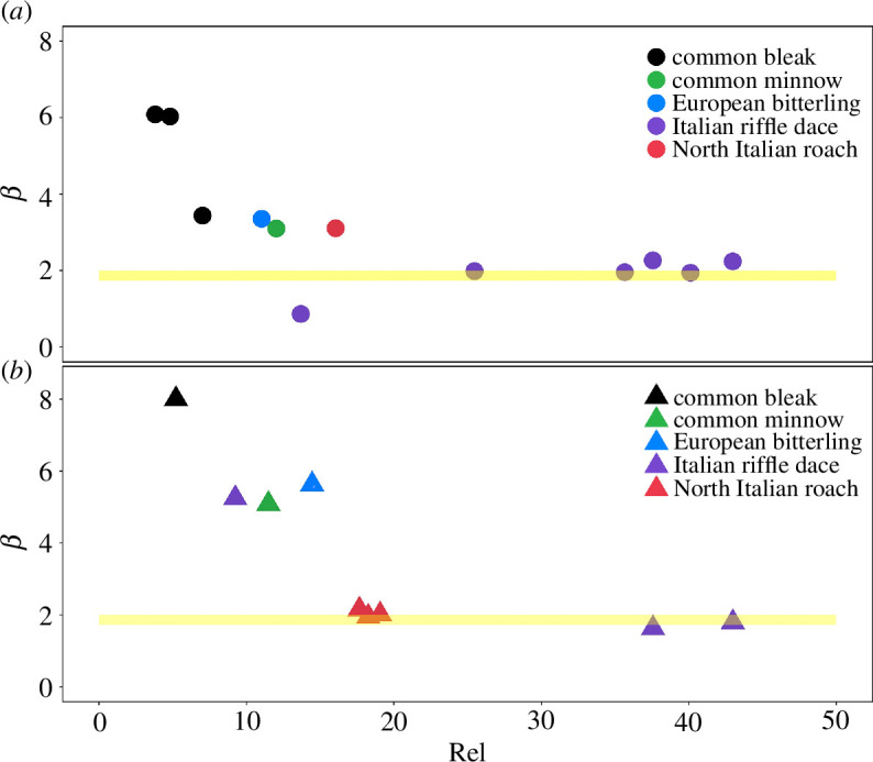
Empirical estimates of scaling exponent β obtained from the linear regression analysis between (a) ln () and ln (Uf) and (b) ln () and ln (Uf) plotted against the ReI, as defined in equation (3.1). The yellow band is the theoretically predicted range of the scaling exponent β, i.e. [1−73−2.0]. Each different colour corresponds to a different fish species as specified in the legend. The repeated data points with the same colour indicate the β values obtained from the fitting of more than one subsampled group related to one single fish species.
5. Discussion
This article presents a theoretical approach that predicts scaling laws linking statistical properties of time-to-fatigue to the mean relative velocity between water and fish, here estimated as Uf. In particular, theory predicts that and , and arguments based upon fish-drag hydrodynamics indicate that the scaling exponent is constrained between 1.73 and 2.00; the overbar-symbol refers to an averaging operator associated with a population of fish of the same species and size, and swimming in water at a given temperature and velocity Uf; the prime symbol identifies variations of around the mean , while k is the moment order and can be any integer greater than one. Dedicated fixed velocity experiments were conducted on five Cypriniformes species, and time-to-fatigue data were used to test the proposed scaling relations for time-to-fatigue mean and variance , by comparing theoretically predicted values of with those estimated from empirical data. Data indicate that empirical estimates of the scaling exponent agree well with theoretical predictions for Italian riffle dace (as estimated from data) or Italian riffle dace and North Italian roach (as estimated from data). Overall, deviations from theoretical predictions tend to reduce noticeably with increasing the ReI (figure 5). This encouragingly supports the validity of the proposed scaling laws; however, it is also true that the trend is only clearly noticeable for Italian riffle dace, for which data span a large range of ReI. Since data for the other four species do not cover the same span (in some cases only one data point is available), there is also a possibility that the extent of the deviations may be species-specific.
It is noteworthy to observe that, at low values of ReI, deviations are not uniformly distributed around the theoretically predicted range but biased towards higher values (i.e. mostly larger than 2). This could be explained as follows: the proposed scaling laws apply to fish swimming in the burst range, i.e. in purely anaerobic conditions but, as mentioned in §4, it is possible that some fish employed both anaerobic and aerobic processes during the trials. Clearly, the probability that individual fish swim using aerobic process reduces with increasing Uf, meaning that Tf outliers (i.e. large values of Tf caused by aerobic swimming) affect estimates of and more in the lower range of Uf than in the higher. Since these outliers contribute to increase both and , they also contribute to enhance the steepness of and versus Uf curves, and hence the values of estimated from the regression analysis.
The theoretical results reported here can have important practical implications. First, they offer advantages for experimental research aiming at quantifying fatigue in fish. In this respect, note that equations (2.5) and (2.9) can be rewritten, in more general form as
| (5.1) |
| (5.2) |
where and are scaling functions which depend mainly on fish species, size and water temperature, and , as discussed, is a well-constrained parameter dictated by theory. This means that, in future studies, it will be possible to explore the statistical behaviour of at only one velocity Uf to retrieve the scaling functions and , hence, significantly reducing experimental efforts devoted to the investigation of endurance in burst swimming. Given the enormous biodiversity reported for fish worldwide and the overwhelming variability in swimming performance associated to it, this result is particularly relevant. Second, equation (5.1) represents a useful tool for fishways’ design and management as it allows to derive the maximum distance a fish can swim before becoming fatigued [3,9,20,24]. Recalling the work by Castro-Santos [24] and Katopodis [9], the maximum distance a fish can swim before fatiguing can be defined as , where is the fish ground speed. Using equation (5.1) for leads to a function that displays a maximum at an optimal relative velocity and hence an optimal ground speed
| (5.3) |
Equation (5.3) indicates that, in the burst swimming range, the maximum distance that a fish can travel is reached at swimming ground speeds of about half of the water flow velocity (recall ). This is clearly true only if fish are fit enough to reach such velocity. If not, the maximum distance is reached at the maximum ground speed they are capable to swim at.
At the optimal velocity, the maximum swimming distance can be estimated as
| (5.4) |
which represents a very important design parameter being the maximum allowed length for a fish passage system [9,21,24].
Finally, we propose that equation (5.4) might offer some biomimicry-inspired insights for the control of underwater robotics, which are now being used for a plethora of applications [69]. Analogously to a fish swimming anaerobically, an underwater robot stops moving (i.e. reaches fatigue) when running out of the energy provided by a battery. Since the theoretical analysis presented in §§2.1 and 2.2 is applicable to any fully submerged solid body that is self-propelled by limited energy resources, equation (5.4), which is a direct consequence of this analysis, indicates that an underwater robot can maximize cruising distances when swimming at ground speeds that are about half of the opposing fluid velocity. Note that underwater robots cannot be charged during operations; therefore, these insights offer a simple strategy to optimize energy consumption in opposing moving waters, as often required in freshwater and marine environments [70].
In conclusion, the main outcome of the present article is a set of theoretically derived scaling laws linking statistical properties of Tf to Ur for burst-swimming fish. These laws are relevant for applications in fishways’ design and to develop bioinspired underwater-robot control. Results from a new and large experimental dataset of five fish species support theoretical predictions, while calling for more experiments from a wider range of fish species and sizes to be carried out, to further establish the general applicability of the proposed scaling laws.
Acknowledgements
The authors would like to acknowledge Paolo Lo Conte and Alessandro Candiotto for their support in electrofishing and fish husbandry, and the Incubatoio di Porte di Pinerolo and the Province of Alessandria for providing access to the hatchery facilities. Additionally, we extend our thanks to Fabio Tarena and Gloria Mozzi for their contributions to the experimental work, and to Andrea Cagninei and Roberto Bosio for their assistance in laboratory activities. C.M. dedicates this paper to Rosanna Farnia who recently passed, sadly bringing with her a lot of unpublished knowledge about fish.
Contributor Information
Muhammad Usama Ashraf, Email: musamaashraf10@gmail.com.
Daniel Nyqvist, Email: daniel.nyqvist@polito.it.
Claudio Comoglio, Email: claudio.comoglio@polito.it.
Vladimir Nikora, Email: v.nikora@abdn.ac.uk.
Andrea Marion, Email: andrea.marion@unipd.it.
Paolo Domenici, Email: paolo.domenici@cnr.it.
Costantino Manes, Email: costantino.manes@polito.it.
Ethics
The experiments were performed with permission from the Protection of Flora and Fauna Department of the Metropolitan City of Turin (authorization D.D. no. 4457 of 29 October 2020) and the Fauna and Ichthyofauna Technical Office of the Alessandria Province (authorization no. 1570 of 19 January 2023), under the provisions of art.2 of the national Decree no. 26/2014 (implementation of Dir. 2010/63/EU).
Data accessibility
The data and code are available in the Zenodo digital repository [71].
Supplementary material is available online [72].
Declaration of AI use
We have not used AI-assisted technologies in creating this article.
Authors’ contributions
M.U.A.: data curation, formal analysis, investigation, methodology, writing—original draft, writing—review and editing; D.N.: investigation, methodology, writing—review and editing; C.C.: funding acquisition, project administration, resources, supervision, writing—review and editing; V.N.: conceptualization, investigation, writing—review and editing; A.M.: conceptualization, investigation, writing—review and editing; P.D.: conceptualization, investigation, methodology, writing—review and editing; C.M.: conceptualization, investigation, methodology, supervision, writing—original draft, writing—review and editing.
All authors gave final approval for publication and agreed to be held accountable for the work performed therein.
Conflict of interest declaration
We declare we have no competing interests.
Funding
The research work was carried out under the funding received from the European Union Horizon 2020 Research and Innovation Programme under the Marie Skłodowska-Curie Actions, Grant Agreement No. 860800.
References
- 1. Castro-Santos T. 2002. Swimming performance of upstream migrant fishes: new methods, new perspectives. Dissertation, University of Massachusetts, Amherst, MA. See https://scholarworks.umass.edu/dissertations/AAI3056208/. [Google Scholar]
- 2. Domenici P, Blake R. 1997. The kinematics and performance of fish fast-start swimming. J. Exp. Biol. 200, 1165–1178. ( 10.1242/jeb.200.8.1165) [DOI] [PubMed] [Google Scholar]
- 3. Katopodis C, Gervais R. 2012. Ecohydraulic analysis of fish fatigue data. River Res. Apps. 28, 444–456. ( 10.1002/rra.1566) [DOI] [Google Scholar]
- 4. Peake S, McKinley RS, Scruton DA. 1997. Swimming performance of various freshwater Newfoundland salmonids relative to habitat selection and fishway design. J. Fish Biol. 51, 710–723. ( 10.1111/j.1095-8649.1997.tb01993.x) [DOI] [Google Scholar]
- 5. Tudorache C, Viaene P, Blust R, Vereecken H, De Boeck G. 2008. A comparison of swimming capacity and energy use in seven European freshwater fish species. Ecol. Freshw. Fish 17, 284–291. ( 10.1111/j.1600-0633.2007.00280.x) [DOI] [Google Scholar]
- 6. Watson J, Goodrich H, Cramp R, Gordos M, Yan Y, Ward P, Franklin C. 2019. Swimming performance traits of twenty-one Australian fish species: a fish passage management tool for use in modified freshwater systems. bioRxiv. ( 10.1101/861898) [DOI] [Google Scholar]
- 7. Barbarossa V, Schmitt RJP, Huijbregts MAJ, Zarfl C, King H, Schipper AM. 2020. Impacts of current and future large dams on the geographic range connectivity of freshwater fish worldwide. Proc. Natl Acad. Sci. USA 117, 3648–3655. ( 10.1073/pnas.1912776117) [DOI] [PMC free article] [PubMed] [Google Scholar]
- 8. Belletti B, et al. 2020. More than one million barriers fragment Europe’s rivers. Nature 588, 436–441. ( 10.1038/s41586-020-3005-2) [DOI] [PubMed] [Google Scholar]
- 9. Katopodis C. 1992. Introduction to fishway design. Manitoba, Canada: Freshwater Institute, Central and Arctic Region Department of Fisheries and Oceans. [Google Scholar]
- 10. Castro-Santos T, Goerig E, He P, Lauder GV. 2022. Applied aspects of locomotion and biomechanics. In Fish physiology, pp. 91–140. Cambridge, MA: Academic Press. ( 10.1016/bs.fp.2022.04.003) [DOI] [Google Scholar]
- 11. Hvas M, Folkedal O, Oppedal F. 2021. Fish welfare in offshore salmon aquaculture. Rev. Aquacult. 13, 836–852. ( 10.1111/raq.12501) [DOI] [Google Scholar]
- 12. Beamish FWH. 1978. Fish physiology, (eds Hoar WS, Randall DJ), vol. 7, 1st edn. London, UK: Academic Press. [Google Scholar]
- 13. Brett JR. 1964. The respiratory metabolism and swimming performance of young sockeye salmon. J. Fish. Res. Bd. Can. 21, 1183–1226. ( 10.1139/f64-103) [DOI] [Google Scholar]
- 14. Hammer C. 1995. Fatigue and exercise tests with fish. Comp. Biochem. Physiol. A Physiol. 112, 1–20. ( 10.1016/0300-9629(95)00060-K) [DOI] [Google Scholar]
- 15. Ashraf MU, et al. 2024. Fish swimming performance: effect of flume length and different fatigue definitions. In Advances in hydraulic research [internet] (eds Kalinowska MB, Mrokowska MM, Rowiński PM), pp. 1–11. Cham, Switzerland: Springer Nature Switzerland. ( 10.1007/978-3-031-56093-4_1). See https://link.springer.com/10.1007/978-3-031-56093-4_1. [DOI] [Google Scholar]
- 16. Tudorache C, O’Keefe RA, Benfey TJ. 2010. Flume length and post-exercise impingement affect anaerobic metabolism in brook charr Salvelinus fontinalis. J. Fish Biol. 76, 729–733. ( 10.1111/j.1095-8649.2009.02513.x) [DOI] [PubMed] [Google Scholar]
- 17. Aedo JR, Otto KR, Rader RB, Hotchkiss RH, Belk MC. 2021. Size matters, but species do not: no evidence for species-specific swimming performance in co-occurring great basin stream fishes. Water 13, 2570. ( 10.3390/w13182570) [DOI] [Google Scholar]
- 18. Farrell AP, Steffensen JF. 1987. An analysis of the energetic cost of the branchial and cardiac pumps during sustained swimming in trout. Fish Physiol. Biochem. 4, 73–79. ( 10.1007/BF02044316) [DOI] [PubMed] [Google Scholar]
- 19. Gregory TR, Wood CM. 1999. The effects of chronic plasma cortisol elevation on the feeding behaviour, growth, competitive ability, and swimming performance of juvenile rainbow trout. Physiol. Biochem. Zool. 72, 286–295. ( 10.1086/316673) [DOI] [PubMed] [Google Scholar]
- 20. Katopodis C, Gervais R. 2016. Fish swimming performance database and analyses. Canadian Science Advisory Secretariat (CSAS) Research Document 2016/002.
- 21. Nikora VI, Aberle J, Biggs BJF, Jowett IG, Sykes JRE. 2003. Effects of fish size, time-to-fatigue and turbulence on swimming performance: a case study of Galaxias maculatus: swimming performance of inanga. J. Fish Biol. 63, 1365–1382. ( 10.1111/j.1095-8649.2003.00241.x) [DOI] [Google Scholar]
- 22. Webb P. 1975. Hydrodynamics and energetics of fish propulsion. Bullettin of the fisheries Research Board of Canada; 190, 1–156. [Google Scholar]
- 23. Videler JJ. 1993. Fish swimming. Dordrecht, The Netherlands: Springer. See http://link.springer.com/10.1007/978-94-011-1580-3. [Google Scholar]
- 24. Castro-Santos T. 2005. Optimal swim speeds for traversing velocity barriers: an analysis of volitional high-speed swimming behavior of migratory fishes. J. Exp. Biol. 208, 421–432. ( 10.1242/jeb.01380) [DOI] [PubMed] [Google Scholar]
- 25. Videler JJ, Wardle CS. 1991. Fish swimming stride by stride: speed limits and endurance. Rev. Fish Biol. Fish. 1, 23–40. ( 10.1007/BF00042660) [DOI] [Google Scholar]
- 26. Castro-Santos T, Sanz-Ronda FJ, Ruiz-Legazpi J. 2013. Breaking the speed limit—comparative sprinting performance of brook trout (Salvelinus fontinalis) and brown trout (Salmo trutta). Can. J. Fish. Aquat. Sci. (ed. Jonsson B), 70, 280–293. ( 10.1139/cjfas-2012-0186) [DOI] [Google Scholar]
- 27. Haro A, Castro-Santos T, Noreika J, Odeh M. 2004. Swimming performance of upstream migrant fishes in open-channel flow: a new approach to predicting passage through velocity barriers. Can. J. Fish. Aquat. Sci. 61, 1590–1601. ( 10.1139/f04-093) [DOI] [Google Scholar]
- 28. Burnett NJ, Hinch SG, Braun DC, Casselman MT, Middleton CT, Wilson SM, Cooke SJ. 2014. Burst swimming in areas of high flow: delayed consequences of anaerobiosis in wild adult sockeye salmon. Physiol. Biochem. Zool. 87, 587–598. ( 10.1086/677219) [DOI] [PubMed] [Google Scholar]
- 29. Nyqvist D, Schiavon A, Candiotto A, Mozzi G, Eggers F, Comoglio C. 2023. PIT-tagging Italian spined loach (Cobitis bilineata): methodology, survival and behavioural effects. J. Fish Biol. 102, 575–580. ( 10.1111/jfb.15289) [DOI] [PubMed] [Google Scholar]
- 30. Taylor EB, McPhail JD. 1985. Burst swimming and size-related predation of newly emerged coho salmon Oncorhynchus kisutch. Trans. Am. Fish. Soc. 114, 546–551. ( 10.1577/1548-8659(1985)114<546:BSASPO>2.0.CO;2) [DOI] [Google Scholar]
- 31. Silva AT, et al. 2018. The future of fish passage science, engineering, and practice. Fish Fish. 19, 340–362. ( 10.1111/faf.12258) [DOI] [Google Scholar]
- 32. Bainbridge R. 1958. The speed of swimming of fish as related to size and to the frequency and amplitude of the tail beat. J. Exp. Biol. 35, 109–133. ( 10.1242/jeb.35.1.109) [DOI] [Google Scholar]
- 33. Bainbridge R. 1960. Speed and stamina in three fish. J. Exp. Biol. 37, 129–153. ( 10.1242/jeb.37.1.129) [DOI] [Google Scholar]
- 34. Hammill E, Wilson RS, Johnston IA. 2004. Sustained swimming performance and muscle structure are altered by thermal acclimation in male mosquitofish. J. Therm. Biol. 29, 251–257. ( 10.1016/j.jtherbio.2004.04.002) [DOI] [Google Scholar]
- 35. Jones PE, Svendsen JC, Börger L, Champneys T, Consuegra S, Jones JAH, Garcia de Leaniz C. 2020. One size does not fit all: inter- and intraspecific variation in the swimming performance of contrasting freshwater fish. Conserv. Physiol. (ed. Cooke S), 8, coaa126. ( 10.1093/conphys/coaa126) [DOI] [PMC free article] [PubMed] [Google Scholar]
- 36. Wardle CS. 1975. Limit of fish swimming speed. Nature 255, 725–727. ( 10.1038/255725a0) [DOI] [PubMed] [Google Scholar]
- 37. Beamish FWH, Howlett JC, Medland TE. 1989. Impact of diet on metabolism and swimming performance in juvenile lake trout, Salvelinus namaycush. Can. J. Fish. Aquat. Sci. 46, 384–388. ( 10.1139/f89-050) [DOI] [Google Scholar]
- 38. Jain KE, Birtwell IK, Farrell AP. 1998. Repeat swimming performance of mature sockeye salmon following a brief recovery period: a proposed measure of fish health and water quality. Can. J. Zool. 76, 1488–1496. ( 10.1139/z98-079) [DOI] [Google Scholar]
- 39. Li J, Lin X, Xu Z, Sun J. 2017. Differences in swimming ability and its response to starvation among male and female Gambusia affinis. Biol. Open 6, 625–632. ( 10.1242/bio.022822) [DOI] [PMC free article] [PubMed] [Google Scholar]
- 40. Penghan LY, Pang X, Fu SJ. 2016. The effects of starvation on fast-start escape and constant acceleration swimming performance in rose bitterling (Rhodeus ocellatus) at two acclimation temperatures. Fish Physiol. Biochem. 42, 909–918. ( 10.1007/s10695-015-0184-0) [DOI] [PubMed] [Google Scholar]
- 41. Quintella BR, Mateus CS, Costa JL, Domingos I, Almeida PR. 2010. Critical swimming speed of yellow- and silver-phase European eel (Anguilla anguilla, L.): critical swimming speed of yellow- and silver-phase European eel. J. Appl. Ichthyol. 26, 432–435. ( 10.1111/j.1439-0426.2010.01457.x) [DOI] [Google Scholar]
- 42. Reidy SP, Kerr SR, Nelson JA. 2000. Aerobic and anaerobic swimming performance of individual Atlantic cod. J. Exp. Biol. 203, 347–357. ( 10.1242/jeb.203.2.347) [DOI] [PubMed] [Google Scholar]
- 43. Goerig E, Castro-Santos T. 2017. Is motivation important to brook trout passage through culverts? Can. J. Fish. Aquat. Sci. 74, 885–893. ( 10.1139/cjfas-2016-0237) [DOI] [Google Scholar]
- 44. Plew DR, Nikora VI, Larned ST, Sykes JRE, Cooper GG. 2007. Fish swimming speed variability at constant flow: Galaxias maculatus. N. Z. J. Mar. Freshw. Res. 41, 185–195. ( 10.1080/00288330709509907) [DOI] [Google Scholar]
- 45. Anderson EJ, McGillis WR, Grosenbaugh MA. 2001. The boundary layer of swimming fish. J. Exp. Biol. 204, 81–102. ( 10.1242/jeb.204.1.81) [DOI] [PubMed] [Google Scholar]
- 46. Lighthill MJ. 1960. Note on the swimming of slender fish. J. Fluid Mech. 9, 305–317. ( 10.1017/S0022112060001110) [DOI] [Google Scholar]
- 47. Lighthill MJ. 1969. Hydromechanics of aquatic animal propulsion. Annu. Rev. Fluid Mech. 1, 413–446. ( 10.1146/annurev.fl.01.010169.002213) [DOI] [Google Scholar]
- 48. Lighthill MJ. 1970. Aquatic animal propulsion of high hydromechanical efficiency. J. Fluid Mech. 44, 265. ( 10.1017/S0022112070001830) [DOI] [Google Scholar]
- 49. Lighthill MJ. 1971. Large-amplitude elongated-body theory of fish locomotion. Proc. R. Soc. Lond. B. 179, 125–138. ( 10.1098/rspb.1971.0085) [DOI] [Google Scholar]
- 50. Gazzola M, Argentina M, Mahadevan L. 2014. Scaling macroscopic aquatic locomotion. Nat. Phys. 10, 758–761. ( 10.1038/nphys3078) [DOI] [Google Scholar]
- 51. Saadat M, Fish FE, Domel AG, Di Santo V, Lauder GV, Haj-Hariri H. 2017. On the rules for aquatic locomotion. Phys. Rev. Fluids 2, 083102. ( 10.1103/PhysRevFluids.2.083102) [DOI] [Google Scholar]
- 52. Eloy C. 2012. Optimal Strouhal number for swimming animals. J. Fluids Struct. 30, 205–218. ( 10.1016/j.jfluidstructs.2012.02.008) [DOI] [Google Scholar]
- 53. Kolok AS. 1992. the swimming performances of individual largemouth bass (Micropterus salmoides) are repeatable. J. Exp. Biol. 170, 265–270. ( 10.1242/jeb.170.1.265) [DOI] [Google Scholar]
- 54. Marras S, Claireaux G, McKenzie DJ, Nelson JA. 2010. Individual variation and repeatability in aerobic and anaerobic swimming performance of European sea bass, Dicentrarchus labrax. J. Exp. Biol. 213, 26–32. ( 10.1242/jeb.032136) [DOI] [PubMed] [Google Scholar]
- 55. Freyhof J, Kottelat M. 2007. Handbook of European freshwater fishes. Cornol, Switzerland: Publications Kottelat. See https://portals.iucn.org/library/node/9068. [Google Scholar]
- 56. IUCN . 2023. The IUCN Red List of Threatened Species. Version 2023-1. See https://www.iucnredlist.org.
- 57. Schneider EV, Hasler CT, Suski CD. 2019. Swimming performance of a freshwater fish during exposure to high carbon dioxide. Environ. Sci. Pollut. Res. 26, 3447–3454. ( 10.1007/s11356-018-3849-2) [DOI] [PubMed] [Google Scholar]
- 58. Tudorache C, O’Keefe RA, Benfey TJ. 2010. The effect of temperature and ammonia exposure on swimming performance of brook charr (Salvelinus fontinalis). Comp. Biochem. Physiol. A Mol. Integr. Physiol. 156, 523–528. ( 10.1016/j.cbpa.2010.04.010) [DOI] [PubMed] [Google Scholar]
- 59. Vezza P, Libardoni F, Manes C, Tsuzaki T, Bertoldi W, Kemp PS. 2020. Rethinking swimming performance tests for bottom-dwelling fish: the case of European glass eel (Anguilla anguilla). Sci. Rep. 10, 16416. ( 10.1038/s41598-020-72957-w) [DOI] [PMC free article] [PubMed] [Google Scholar]
- 60. Ashraf MU, Nyqvist D, Comoglio C, Manes C. 2024. The effect of in-flume habituation time and fish behaviour on estimated swimming performance. J. Ecohydraul. 1–9. ( 10.1080/24705357.2024.2306411) [DOI] [Google Scholar]
- 61. Schiavon A, Comoglio C, Candiotto A, Hölker F, Ashraf MU, Nyqvist D. Survival and swimming performance of a small-sized cypriniformes (Telestes muticellus) tagged with passive integrated transponders. J. Limnol. 82. ( 10.4081/jlimnol.2023.2129) [DOI] [Google Scholar]
- 62. Heuer RM, Stieglitz JD, Pasparakis C, Enochs IC, Benetti DD, Grosell M. 2021. The effects of temperature acclimation on swimming performance in the pelagic mahi-mahi (Coryphaena hippurus). Front. Mar. Sci. 8, 654276. ( 10.3389/fmars.2021.654276) [DOI] [Google Scholar]
- 63. Deslauriers D. 2011. Factors influencing swimming performance and behaviour of the shortnose sturgeon (acipenser brevirostrum). MSC thesis, University of New Brunswick, Saint John, Canada. [Google Scholar]
- 64. Jerde CL, Kraskura K, Eliason EJ, Csik SR, Stier AC, Taper ML. 2019. Strong evidence for an intraspecific metabolic scaling coefficient near 0.89 in fish. Front. Physiol. 10, 1166. ( 10.3389/fphys.2019.01166) [DOI] [PMC free article] [PubMed] [Google Scholar]
- 65. R team . 2022. The R Project for Statistical Computing. Vienna, Austria: R Foundation for Statistical Computing. See https:// www.R-project.org. [Google Scholar]
- 66. Wickham H, François R, Henry L, Müller K, Vaughan D, Posit Software, PBC . 2023. dplyr: A Grammar of Data Manipulation. See https://cran.r-project.org/package=dplyr.
- 67. Wickham H, et al. 2024. Ggplot2: create elegant data visualisations using the grammar of graphics. See https://cran.r-project.org/package=ggplot2.
- 68. Mayer M. 2023. Confintr: confidence intervals https://cran.r-project.org/package=confintr
- 69. Cui Z, Li L, Wang Y, Zhong Z, Li J. 2023. Review of research and control technology of underwater bionic robots. Intell. Mar. Technol. Syst. 1, 7. ( 10.1007/s44295-023-00010-3) [DOI] [Google Scholar]
- 70. Li X, Yu S. 2023. Comparison of biological swarm intelligence algorithms for AUVs for three-dimensional path planning in ocean currents’ conditions. J. Mar. Sci. Technol. 28, 832–843. ( 10.1007/s00773-023-00960-7) [DOI] [Google Scholar]
- 71. Ashraf MU, Nyqvist D, Comoglio C, Nikora V, Marion A, Domenici P, Manes C. 2024. Time-to-fatigue data for five cypriniformes fish species and R script for data analysis. Zenodo. https://zenodo.org/records/13275592
- 72. Ashraf MU, Nyqvist D, Comoglio C, Nikora V, Marion A, Domenici Pet al. 2024. Data from: Decoding burst swimming performance: a scaling perspective on time-to-fatigue. Figshare. ( 10.6084/m9.figshare.c.7423801) [DOI] [PubMed]
Associated Data
This section collects any data citations, data availability statements, or supplementary materials included in this article.
Data Availability Statement
The data and code are available in the Zenodo digital repository [71].
Supplementary material is available online [72].