

Abstract
We explore how nuclear shut-downs in the United States could affect air pollution, climate and health with existing and alternative grid infrastructure. We develop a dispatch model to estimate emissions of CO2, NOx and SO2 from each electricity-generating unit, feeding these emissions into a chemical transport model to calculate effects on ground-level ozone and fine particulate matter (PM2.5). Our scenario of removing nuclear power results in compensation by coal, gas and oil, resulting in increases in PM2.5 and ozone that lead to an extra 5,200 annual mortalities. Changes in CO2 emissions lead to an order of magnitude higher mortalities throughout the twenty-first century, incurring US$11–180 billion of damages from 1 year of emissions. A scenario exploring simultaneous closures of nuclear and coal plants redistributes health impacts and a scenario with increased penetration of renewables reduces health impacts. Inequities in exposure to pollution are persistent across all scenarios—Black or African American people are exposed to the highest relative levels of pollution.
The United States relies on nuclear and coal for 38% of its electricity generation1. Analysis of pathways for the United States to reach a net-zero carbon emissions energy grid focus on reduction of fossil fuels and increased use of renewable energy2. Nuclear power, whose use is projected to decline in the future, has historically provided many parts of the United States with low-emission (both direct and indirect) energy that has had lower health- and accident-related illnesses and deaths when compared to coal, gas and oil3. Nuclear power has also been evaluated for its role in reducing historical carbon emissions at the global scale4,5 but it remains of public and government concern due to potential safety risks. At the same time, coal has long been one of the highest polluting sources of electricity, contributing to hundreds of thousands of premature deaths globally each year (other fossil fuel use brings this up to millions of deaths)6,7 and 3,100 premature deaths in the United States in 2016 (a large improvement from an estimated 30,000 premature deaths in 2000)8. Even without substantial new climate action, it is still estimated that coal use will decline rapidly over the coming decades. In contrast, renewable sources of electricity such as wind and solar are expected to grow over the coming decades1. There is little comprehensive work on the potential air quality impacts of reducing the role of nuclear power in the United States energy system and how this reduction will interact with other aspects of the energy transition.
Recent closures of nuclear power plants are due to a combination of economic impracticability because of inexpensive gas9, as well as health and safety concerns, and have historically led to increased use of fossil fuels to fill the gap in energy production. The Zero Emission Nuclear Power Production Tax Credit of the Inflation Reduction Act provides tax credits to financially incentivize utilities to continue the use of nuclear power between 2024 and 2032, which may push back the shut-down timeline for nuclear power plants and encourage the development of small modular reactors10. This does not guarantee the long-term use of these nuclear plants, so it is important to quantify the effect that maintaining versus shutting them down could have on health and the climate, particularly in the context of renewable energy growth and fossil fuel closures.
These recent shut-downs include the Indian Point Energy Center second reactor, which was shut down in April 2021 because of environmental and safety concerns due to its proximity to New York City11. Browns Ferry and Sequoyah nuclear power plant shut-downs in 1985 led to increased coal use12, as determined by regressions comparing power plant level production in the Tennessee Valley Area before and after the nuclear plant closures. Using similar regressions to assess generation by plants before and after the San Onofre Nuclear Plant (California) shut-down in 2012, ref. 13 found nuclear power plant closure led to increased gas use, as well as increased costs of electricity generation. Recent work has shown that phase-out of nuclear power from 2011 to 2017 in Germany led to replacement by fossil fuels14.
The fossil fuels that have historically replaced nuclear power have emissions that contribute to air pollution and climate change. Fossil fuel plants emit nitrogen oxides (NOx) and sulfur dioxide (SO2), both of which are precursors for fine particulate matter (PM2.5) and NOx is a precursor for ozone15. Air pollution due to ozone and PM2.5 is associated with adverse health outcomes and premature mortality16,17. Concerns that the pending closure of the Diablo Canyon nuclear power plant by 2025 could result in increased use of fossil fuels and associated climate impacts18, and compromise energy grid stability, led to the decision to extend its lifetime by 5 years.
Previous work has only addressed subnational-level response to nuclear power shut-downs or has quantified regional and globally averaged avoided mortalities from nuclear power use. Using the InMAP reduced form model, ref. 19 found that the shut-down of three nuclear power plants in the Pennsylvania–New Jersey–Maryland region led to increases in PM2.5 resulting in 126 additional mortalities. Another study5 quantified the global historical prevented mortalities and CO2 emissions due to historical and potential future nuclear power generation, using average mortality rates and CO2 emissions rates by electricity type. They project mortalities and CO2 emissions based on energy projections by the UN International Atomic Energy Agency out to 2050, finding that 4.39–7.04 million deaths would be prevented by using nuclear power, rather than fossil fuels, due to lower emissions of air pollutants. Previous work also has not consistently accounted for the potential growth of renewable energy, which has been shown to replace the use of fossil fuels20.
Here, we construct four national-scale energy scenarios to better characterize the nationwide system response to nuclear shut-downs. We compare four scenarios in which: (1) the United States shuts down all nuclear power (no nuclear), (2) the United States shuts down all coal and nuclear power (no nuclear + no coal), (3) the United States shuts down all nuclear and expands renewable capacity to 2030 Energy Information Administration (EIA) regional projections (no nuclear + renewables) and (4) the United States continues at an existing baseline (base). These scenarios allow us to characterize a maximum potential impact of nuclear shut-downs, explore the dynamics of the energy system in response to the loss of coal and nuclear power, evaluate the role of expanding renewables in place of nuclear power and estimate the impacts on climate and human health. Although all nuclear power will not realistically shut down at once and nor will all coal and nuclear power, this study identifies regions with high risk due to a system-wide response to closures. This is further explored by quantifying the effect of replacing one low-emissions (direct and indirect) source of energy (nuclear) with another (wind and solar). We examine the impact of these scenarios on people of different races and ethnicities, as prior research has shown that people of colour are not only disproportionately exposed to air pollution21–24 but also experience up to three times the impact of PM2.5 on mortality16,25. To do this, we couple an energy grid/dispatch model and a chemical transport model to calculate the economic and health impact of both climate and air quality changes and further quantify shifts in exposure amongst different communities.
Energy grid response and emission changes
There is more fossil fuel generation in no nuclear than in the base. In the base, gas is 32% of the energy generation, coal is 31% and oil is <1%; in no nuclear, gas is 39% of the energy generation, coal is 45% and oil is <1%. Figure 1b shows the differences in fossil fuel use, which are largely concentrated in the Eastern United States because of the high concentration of nuclear power there. The interconnected nature of the energy grid can be seen through the differences in the location of increased fossil fuel generation—when nuclear power plants in one county or state are not available, fossil fuel generators in other counties and states can make up the difference in demand. We calculate the ability to meet demand under each scenario and estimate the gaps, showing that the United States does not have the necessary capacity to close all of its nuclear power and meet current demand. In no nuclear, this gap occurs in Texas during the summer—Texas has already faced increasing issues with the ability of its electricity grid to meet demand during severe weather26, so an additional loss in production could exacerbate uncertainty in the region. In no nuclear + no coal (Fig. 1c) there is an increase in gas and oil use and the electricity grid cannot meet demand in more than half of the regions in the United States (Supplementary Discussion). Increased availability of renewables in no nuclear + renewables leads to most of the lost load being taken up by wind and solar (Fig. 1d).
Fig. 1 |. Maps of differences in annual energy generation by EGU across our scenarios.
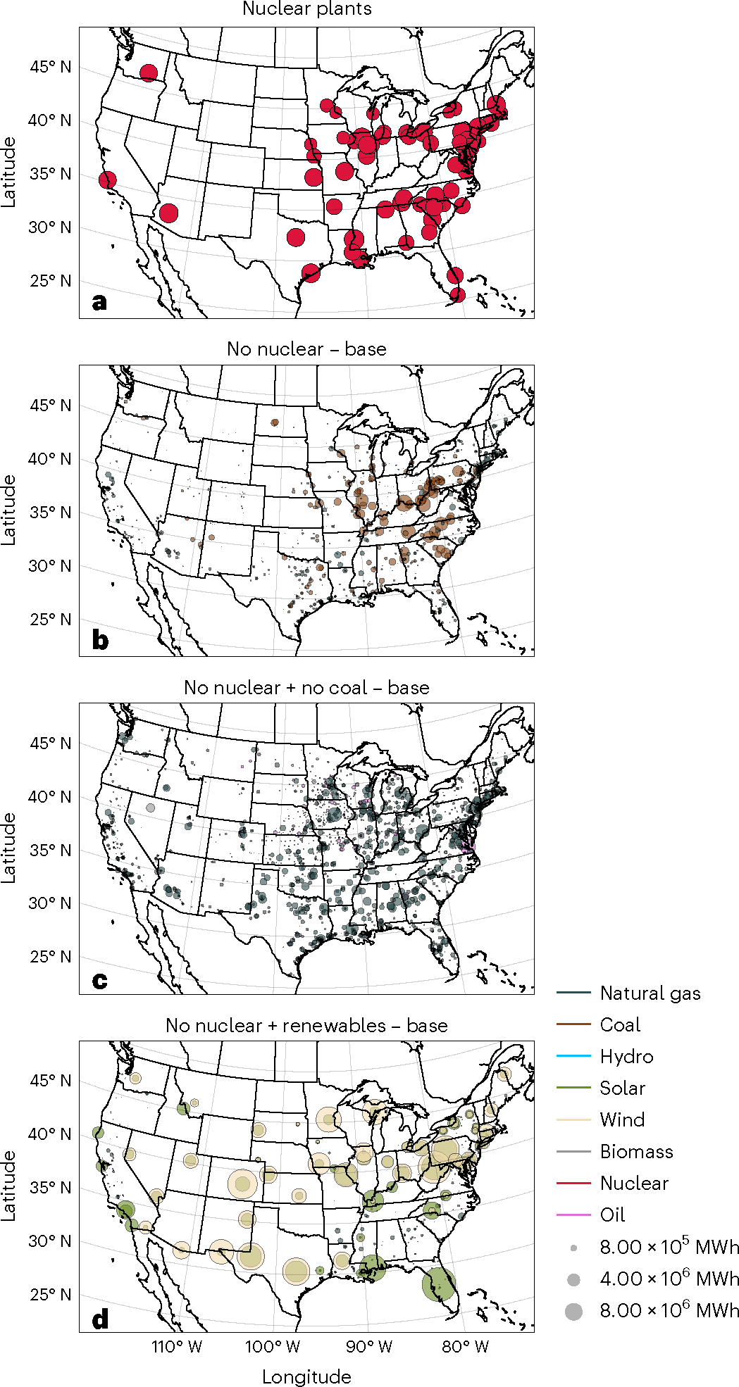
a–d, Annual energy production (MWh) by each nuclear plant in the base (a), difference in annual energy production (MWh) by unit in no nuclear compared to the base (b), difference in annual energy production by unit (MWh) in no nuclear + no coal compared to the base (c) and difference in annual energy production (MWh) by unit in no nuclear + renewables compared to the base (d). In b, c and d, we only plot the increases, which excludes nuclear power from b and d and nuclear and coal power from c.
Higher fossil fuel use in no nuclear leads to increases in emissions of NOx, SO2 and CO2, compared to the base. There are 42% more NOx, 45% more SO2 and 41% more CO2 emissions than in the base (Supplementary Fig. 3). The largest differences in NOx and SO2 concentrations occur in the Eastern United States and during the summer due to changes in emissions in these locations (Supplementary Fig. 7).
Pollution and health impacts
Figure 2 shows that annual average PM2.5 concentrations are higher nationwide under no nuclear compared to the base. These variations in PM2.5 are driven by the changes in NOx and SO2 emissions. PM2.5 concentrations are larger in no nuclear than the base throughout the Eastern United States during both summer and winter. The concentration differences between no nuclear and the base are larger in the summer than in the winter (Supplementary Fig. 10).
Fig. 2 |. Map of changes in concentration and mortalities in no nuclear compared to the base.

a–d, Changes in April–September MDA8 ozone concentrations (a) and annual average PM2.5 concentrations (c) and the subsequent change in mortalities per 1 million people due to no nuclear compared with the base (b,d, respectively).
Ozone season (April–September, as defined by ref. 17), local maximum daily average 8 h (MDA8) ozone concentrations are larger on average nationwide under no nuclear than in the base scenario. The Eastern United States experiences higher changes in ozone than the West.
We calculate two mortality metrics—those due to air quality exposure and those due to CO2 emissions. Those due to changes in air quality are total annual mortalities, expected to be incurred in the year of exposure as a result of concurrent emissions. Mortalities calculated due to changes in CO2 are integrated mortalities, expected to be incurred throughout the twenty-first century as a result of the climate impacts from a single year’s emissions. Both metrics are calculated on the basis of one single year of emissions; if a scenario were to persist for more than a single year, mortalities would compound.
The differences between all-cause mortality for ages 25+ yr due to changes in PM2.5 and April–September MDA8 ozone concentrations in no nuclear compared with the base are shown in Fig. 2. Due to changes in PM2.5 concentrations in no nuclear compared with the base, there are 3,600 (95% confidence interval (CI), 2,800–4,600) additional premature mortalities. Most of the increase in mortalities is in the Eastern United States, due to the higher PM2.5 in the Eastern United States than the Western United States. Yearly mortalities due to the change in April–September MDA8 ozone concentrations are larger in the Eastern United States, where no nuclear has 1,600 (95% CI, 800–3,100) additional premature mortalities as compared to the base.
We use the mortality cost of carbon (MCC)27 to calculate the integrated mortalities until 2100 of the yearly CO2 emissions. The MCC has a baseline and optimal climate outcome, with low, central and high mortality estimates. Under a central estimate for the optimal and baseline scenario, CO2 emissions due to no nuclear lead to an additional 78,000 or 170,000 mortalities throughout the rest of the twenty-first century compared to the base (−130,000 or −160,000 to 380,000 or 500,000 mortalities under low and high estimates).
Impact monetization
Using regulatory approaches28, we monetize the annual impact of the increased carbon emissions as well as the health impacts of the changes in air quality from no nuclear compared to the base. We use a value of statistical life (VSL), as defined by the Environmental Protection Agency (EPA) to monetize the changes in mortalities due to air quality, and a social cost of carbon (SCC) to monetize the damages due to changes in carbon emissions, both of which are expressed in year 2007 US dollars.
We calculate the annual cost of mortalities due to changes in April–September MDA8 ozone and annual mean PM2.5 using the EPA’s current estimate for the VSL of US$7.4 million (in year 2007 US dollars)29. There are US$40 billion in monetized externalities due to air pollution (US$12 billion due to ozone and US$28 billion due to PM2.5) for the no nuclear scenario.
We also quantify a range of values for the monetized social impact of the change in carbon emissions according to the 2020 government SCC (in year 2007 US dollars) across a range of discount rates and future climate scenarios30 to account for uncertainty. We also use the recent higher estimates of an SCC from ref. 31. The mean monetized SCC due to 1 year of emissions from no nuclear is between US$11 billion and US$180 billion (for discount rates of 5% and 1.5%, respectively). This is probably an underestimate of the total impact of greenhouse gas emissions from this transition, as we do not include changes in methane emissions due to the high uncertainties in emission factors (Supplementary Fig. 1). Overall, 1 year of emissions from no nuclear leads to costs between US$51 billion and US$220 billion (in year 2007 US dollars) due to both climate and health impacts nationwide.
Distributional consequences and system analysis
We quantify the difference in population-weighted PM2.5 and ozone exposure amongst racial and ethnic groups under no nuclear compared to the base, finding that Black or African American people experience the largest difference in both exposure and mortalities. The distribution of mortalities by race and ethnicity is right-skewed for all but Black or African American people, who have a much more uniform distribution of exposure, meaning that a much smaller portion of Black or African American people experience the lowest levels of pollution due to these shut-downs. Figure 3 shows the percentage of the population by county of each race and ethnicity that has a given change in mortality rate due to PM2.5 or ozone (see Fig. 3 for histograms of exposure by race and ethnicity and Supplementary Tables 3–6 for exposure and mortality data).
Fig. 3 |. Distribution of exposure and mortalities by race and ethnicity for each county in no nuclear.

a–h, Percentage of each race and ethnicity (Black or African American (a,f,k,p), Hispanic or Latino (b,g,l,q), American Indian or Alaska Native (c,h,m,r), White (d,i,n,s) and Asian or Pacific Islander (e,j,o,t)) with a given summer annual average PM2.5 (a–e) and April–September MDA8 ozone exposure (k–o) and related mortality rate by county (f–j and p–t, respectively), weighted by population for the difference between no nuclear and the base (f–j and p–t, respectively). Mean population-weighted exposure and mortalities are indicated by the vertical line.
We use the no nuclear + no coal and no nuclear + renewables scenarios to explore variations in the system response if both fossil fuels and nuclear are phased out simultaneously or if nuclear is replaced by renewables. In no nuclear + no coal, gas provides 75% of the electricity generation and oil provides 1.9% and there are 194% more NOx emissions, 23% less SO2 emissions and 5% more CO2 emissions than in the base. In no nuclear + renewables, gas provides 33% of electricity generation (a 1.5% increase from the base), coal provides 34% (an 8.6% increase from the base) and solar and wind provide 7.6% and 16% of generation, respectively (a 1,750% and 158% increase from the base).
No nuclear + no coal illustrates that oil and gas, particularly plants with high emissions factors that are currently rarely used, could be increasingly called upon to meet demand in the electricity system if there is not adequate planning to replace nuclear and coal plants as they shut down. Not only does the generation and emissions from these plants become a larger percentage of the overall system but there is a net increase in emissions of NOx, SO2 and CO2 due to the reliance on these plants. As with no nuclear, Black or African American people have the largest increase in exposure to pollution due to the shut-down of both nuclear and coal power (Fig. 4).
Fig. 4 |. Distribution of exposure and mortalities by race and ethnicity for each county in no nuclear + no coal.

a–h, Percentage of each race and ethnicity (Black or African American (a,f,k,p), Hispanic or Latino (b,g,l,q), American Indian or Alaska Native (c,h,m,r), White (d,i,n,s) and Asian or Pacific Islander (e,j,o,t)) with a given annual average PM2.5 (a–e) and April–September MDA8 ozone exposure (k–o) and related mortality rate by county (f–j and p–t, respectively), weighted by population for the difference between no nuclear + no coal and the base. Mean population-weighted exposure and mortalities are indicated by the vertical line.
If additional renewable capacity is made available alongside the shut-down of nuclear plants, as in no nuclear + renewables, the percentage of energy generation by solar and wind approximately replaces the loss in nuclear generation. However, this does not preclude health impacts, as there are increases in mortalities due to PM2.5 and ozone in the Eastern half of the United States, with decreases in the Western United States. There are net 260 additional premature mortalities in this scenario (980 additional mortalities due to PM2.5 and a decrease in 720 mortalities due to ozone), which is less than if nuclear plants are shut down without an alternative clean source of energy (Fig. 5). However, the lack of an overall reduction in mortalities indicates that just replacing nuclear power with renewables will not improve air quality nationwide. This scenario leads to amplification of existing inequities in exposure to pollution, as Black or African American people have the largest mean increase in exposure and subsequent mortalities due to PM2.5 and the lowest mean decrease in exposure and subsequent mortalities due to ozone (Fig. 6).
Fig. 5 |. Map of changes in concentration and mortalities in no nuclear + no coal and no nuclear + renewables compared to the base.

a–h, Changes in April–September MDA8 ozone (a,b) and annual average PM2.5 concentrations (e,f) and the respective subsequent change in mortalities per 1 million people (c,d and g,h).
Fig. 6 |. Distribution of exposure and mortalities by race and ethnicity for each county in no nuclear + renewables.

Percentage of each race and ethnicity (Black or African American (a,f,k,p), Hispanic or Latino (b,g,l,q), American Indian or Alaska Native (c,h,m,r), White (d,i,n,s) and Asian or Pacific Islander (e,j,o,t)) with a given annual average PM2.5 (a–e) and April–September MDA8 ozone exposure (k–o) and related mortality rate by county (f–j and p–t, respectively), weighted by population for the difference between no nuclear + renewables and the base. Mean population-weighted exposure and mortalities are indicated by the vertical line.
In both no nuclear + no coal and no nuclear + renewables, population-weighted exposure to both PM2.5 and ozone and related mortality rates are higher for those living in a county with a nuclear plant that was shut down, than those living in counties that did not have nuclear plants (Supplementary Fig. 12). This is in contrast to no nuclear, where those living in counties with or without nuclear power plants are approximately equivalently impacted by the resulting shift in air quality (Supplementary Fig. 12). Supplementary Tables 7–10 show the detailed mortality and population-weighted exposure rates for both county types.
Coal plant shut-downs disproportionately benefit those living in counties with coal plants; these counties have lower mortality rates due to changes in PM2.5 and ozone than do non-coal counties. In no nuclear + no coal compared to the base, counties with coal power plants that are shut down have lower increases in mortalities per 1 million people due to PM2.5 and ozone (12 and 18, respectively) than those living in counties that do not have a coal plant that is shut down (12 and 21, respectively) (Supplementary Fig. 11). Furthermore, those living in counties with coal plants have lower mortality rates per 1 million people due to changes in PM2.5 and ozone in no nuclear + no coal than in no nuclear, compared to the base (Supplementary Fig. 11).
Discussion and conclusion
Closure of all nuclear power plants across the United States (no nuclear) leads to more mortalities due to air pollution and climate compared to a baseline scenario (base). There are an additional 5,200 annual mortalities due to changes in PM2.5 and ozone under no nuclear. These health impacts are a similar order of magnitude as those estimated in studies on the impact of proposed carbon policies such as the Clean Power Plan on air quality (3,500 avoided premature mortalities were projected to result if the Clean Power Plan were implemented)32. Compared to the base, there is a central estimate of 78,000–170,000 additional mortalities over the century due to the changes in CO2 emissions from 1 year of no nuclear. These mortalities compound with each year of continued emissions. Our scenarios do not account for changes in demographics over time, or changes in electricity demand, which is expected to increase with the electrification of transportation and buildings, thus putting more burden on the system if nuclear power is shut down.
We show here how local- or utility-scale decisions to use certain energy sources impact air quality at a broader regional and national level. These impacts are larger when the electricity grid relies more on fossil fuels. Nuclear power is not without risk, as it has had considerable historical impacts on human health and the environment, which has led to concern for those living near power plants or working in the industry. There is extensive research on the social and historical context of the nuclear power industry, which points to high-risk accidents, health impacts of living near the radiation of a plant and waste management and inadequate safety measures from uranium mining, which has had particularly negative impacts within the Navajo Nation, as some of the safety concerns with continued use of nuclear power33–36. We do not include the impacts of uranium mining in this work but it is an important component of environmental and energy injustices and future work could focus on life cycle analyses to include these other impacts.
If coal is retired alongside nuclear or renewable capacity is increased, those in counties with nuclear plants that are shut down are disproportionately harmed by the resulting shift in pollution. In contrast, those living in counties with coal power plants benefit the most from closures of coal power plants (Supplementary Figs. 11 and 12). The development of renewable capacity alongside nuclear plant closures will not exactly mimic our modelling scenario in no nuclear + renewables. This scenario does show that to reduce air quality and climate impacts, cost-competitive renewables should be built to replace nuclear closures, particularly where fossil fuels would otherwise fill the gap in generation and in locations that contribute to inequities in exposure to pollution.
All of our scenarios disproportionately harm Black or African American people, substantiating previous work that shows the need for energy policy to consider more than just cost optimization37. This work can be used by decision-makers responsible for the maintenance or closure of nuclear plants as a component of their risk assessments for different communities, and to inform plans to mitigate impacts from pollution.
Methods
Scenario development
We combine an energy grid model (US-EGO) and a chemical transport model (GEOS-Chem) to assess the impact of nuclear plant shut-downs in the United States. This method is a typical tool in regulatory impact analysis and has been used across multiple studies38–40.
We create a total of seven scenarios, 1–4 are analysed in the main text and 5–7 are used in the Supplementary Methods for evaluation of US-EGO and GEOS-Chem. Five scenarios are generated through US-EGO: (1) a no nuclear scenario (no nuclear), (2) a no nuclear or coal scenario (no nuclear + no coal), (3) a no nuclear with renewable capacity expanded to 2030 projections (no nuclear + renewables), (4) a base scenario (base) and (5) a modification of the base scenario where emissions are modified to match regional data from the EPA’s Emissions and Generation Resource Integrated Database (eGRID). The other two scenarios use existing emissions inventories: (6) a scenario using the National Emissions Inventory (NEI) from 2011 and (7) a scenario using the most recently available NEI data from 2016. Table 1 shows the seven scenarios and associated data; scenario development and the evaluation of US-EGO and GEOS-Chem are discussed in Supplementary Methods.
Table 1 |.
GEOS-Chem simulations
| Short name | Explanation | Data source/US-EGO simulated | Use in paper |
|---|---|---|---|
| No nuclear | Shut-down of all nuclear power | US-EGO no nuclear | Main text analysis |
| No nuclear+no coal | Shut-down of all nuclear and coal power | US-EGO no nuclear + no coal scenario | Main text analysis |
| No nuclear+renewables | Shut-down of all nuclear power and expansion of renewable capacity to 2030 EIA projections | US-EGO no nuclear + renewables scenario | Main text analysis |
| Base | 2016 baseline | US-EGO base scenario | Main text analysis |
| NEI2011 | GEOS-Chem default NEI in year 2011 | NEI 2011 | Supplementary model evaluation |
| NEI 2016 | Updated NEI for the GEOS-Chem model based on new 2016 data from the EPA55 | NEI 2016 | Supplementary model evaluation |
| eGRID | 2016 baseline modified so that regional total emissions match that of the eGRID | US-EGO modifying regional totals to match eGRID | Supplementary model evaluation |
Associated PM2.5 and ozone-related premature mortalities due to changes in the electricity grid are calculated according to concentration–response functions from ref. 41 and ref. 17, respectively. We calculate the change in mortalities across the twenty-first century due to one year’s CO2 emissions through an MCC27. The monetized social impact of carbon is calculated using 2020 SCC across a range of discount rates30,31 and the monetized health impacts are calculated using the VSL29.
Energy grid optimization model
We extend and evaluate the US-EGO based on ref. 42. US-EGO estimates hourly emissions of NOx, SO2 and CO2 from every power plant in the United States. Model evaluation can be found in Supplementary Methods and Supplementary Figs. 1 and 3. Data for this model are from the EPA’s National Electric Energy Data System (NEEDS) model v.5.16 (ref. 43), which provides the location, generation costs, capacity, electricity demand and emissions factors for every energy generating unit (EGU) in the United States. We assume no change in demand beyond the year 2016. We use these data to set up a cost optimization, which is based on the Security Constrained Unit Commitment model44 for the energy market. This optimization is solved such that the supply of energy satisfies demand at every hour in 64 regions (as based on NEEDS), allowing for transmission between certain regions. It runs across time periods with (1) generation for generator at cost with total generators and (2) transmission power between regions and at cost . We run the model for 8,760 h throughout the year, separately optimizing at each time step42.
| (1) |
Constraints for the model can be found in Supplementary Methods.
We take the hourly output of generation from the model and calculate the hourly emissions of and by
| (2) |
where is the emissions factor specific to that EGU. These hourly emissions are mapped onto a 0.5° × 0.625° grid to allow for their input into the chemical transport model, GEOS-Chem.
To generate the no nuclear scenario, we remove all nuclear power plants from the possible set of EGUs. US-EGO requires sufficient supply to meet demand to calculate a solution to its optimization. To close the optimization in no nuclear, we implement additional zero emissions generation capacity which is available in each of the 64 regions. The pricing of the additional generation we implement is high, such that it is only triggered when the existing grid is at complete capacity. With a shut-down of all nuclear power, southeastern Texas demand exceeds supply for 20 h in the month of May and we discuss the closure of this gap in Supplementary Methods. To generate the no nuclear + no coal scenario, we remove all coal and nuclear power plants from the possible set of EGUs. In this scenario, 35 regions43 have to use additional generators to meet demand (Supplementary Methods). The no nuclear + renewables scenario is generated by removing all nuclear power plants from the possible set of EGUs and adding capacity as projected by the EIA for 25 electricity market module regions. These regions contain our 64 NEEDS regions, so we allow the total capacity across all NEEDS subregions to sum to the total projected capacity in the larger EIA region. When additional renewable capacity as projected for 2030 by the EIA is made available, supply meets demand at all times. Maps of EGU annual generation for the base, no nuclear, no nuclear + no coal and no nuclear + renewables scenarios are shown in Supplementary Fig. 2.
Chemical transport model
We use the GEOS-Chem model v.13.2.1 (ref. 45) to simulate SO2, NOx, PM2.5 and ozone concentrations. GEOS-Chem is a global three-dimensional chemical transport model that includes aerosol chemistry46 and tropospheric oxidant chemistry47. We use a global horizontal resolution of 4° × 5° to create boundary conditions for a nested North American run with horizontal resolution of 0. 5° × 0.625° between 140° and 40° W and 10° and 70° N (ref. 48). This resolution is similar to that of other studies examining air quality impacts and disparities (for example, refs. 41,49–51). GEOS-Chem is driven by meteorological data from the MERRA-2 re-analysis52. Emissions data come from the Harvard-NASA Emission Component53. We use 6 months for spin-up and we analyse daily concentration outputs for the year of 2016.
Within Harvard-NASA Emission Component, we make a few key modifications to the inputs of emissions for EGUs. For our NEI 2011 simulation, the EGU emissions for GEOS-Chem are from the 2011 NEI that are scaled to the relevant year as described in the GEOS-Chem wiki54. In the NEI 2016 simulation, we use recently developed emissions inventories for the NEI in 201655. The base, no nuclear, no nuclear + no coal and no nuclear + renewables scenarios all use emissions profiles of SO2 and NOx created through the relevant US-EGO model simulation. The eGRID simulation uses the base US-EGO run, modified such that the total emissions in each of the 64 NEEDS regions match that of the data from the eGRID56 SO2 and NOx emissions gridded onto a 0.5° × 0.625° grid. In the base, no nuclear, no nuclear + no coal, no nuclear + renewables, eGRID and NEI 2016 scenarios, all emissions other than the EGU SO2 and NOx emissions are from the 2016 NEI emission inventory. Comparisons of GEOS-Chem output to observational data are further discussed in Supplementary Methods and are shown in Supplementary Figs. 4, 5 and 6 and Supplementary Tables 1 and 2. Supplementary Figs. 9 and 10 show the annual mean concentration of PM2.5 and ozone for each of the seven scenarios and their seasonal difference from the base, respectively. Supplementary Fig. 8 shows ozone regimes for each of the scenarios, providing insight into locations that have decreases in ozone despite increases in NOx concentrations due to NOx titration57.
Health impact assessment
We calculate the differences in annual mean PM2.5 concentrations between no nuclear, no nuclear + no coal or no nuclear + renewables and the base. Mortalities due to changes in PM2.5 exposure are calculated using the concentration–response functions from a recent meta-analysis of the association between PM2.5 and mortality41. For each grid box, we calculate , the long-term PM2.5 concentration–response, as
| (3) |
where is based on Fig. 2 in ref. 41, such that its value depends on is the base scenario and is no nuclear, no nuclear + no coal or no nuclear + renewables scenario and is the annual average change in PM2.5 between scenarios and . We calculate the 95% CI for based on this same method, using the upper and lower bounds on the 95% CI from ref. 41
We calculate the incidence, , for each grid box as
| (4) |
On the basis of the change in concentration and incidence, we calculate the change in all-cause mortality for each GEOS-Chem grid cell as7
| (5) |
where is the affected population, for which we use the Gridded Population of the World data58 and is the state-level baseline all-cause mortality numbers taken from the 2017 Global Burden of Disease Study59, using state-level population data from the United States Census Bureau Demographic Analysis Data to calculate the mortality rate60. All mortalities are calculated for the population aged 25+ yr.
For ozone, we similarly quantify the differences in concentration between the base and no nuclear, no nuclear + no coal or no nuclear + renewables. Mortalities due to ozone changes are calculated following the methods used in the latest Regulatory Impact Analysis for the Final Revised CSAPR by the EPA17,61. From this, we calculate three values (the mean and 95% CI) for the long-term ozone concentration–response as , where RR = 1.02 [1.01, 1.04] is the relative risk per 10 ppb () increase in April–September ozone in a two-pollutant model accounting for PM2.5 (ref. 17). We use April–September MDA8 ozone concentrations, defined as the maximum of the local rolling 8 h average ozone from April to September. We calculate a change in mortality for each and grid cell as
| (6) |
In which the mean mortality is based on the mean and our 95% CI mortality is based on the 95% CI for is the change in ozone for each grid cell.
We aggregate our gridded PM2.5 and ozone data to county levels using area-weighted averages (using the python module, xesmf62) across the United States. We use United States Census Bureau Demographic Analysis Data for the year 201663 to attribute changes in mortality at the county level based on race (Asian or Pacific Islander, American Indian, Black or African American and White) and Hispanic origin/ethnicity (not Hispanic or Latino and Hispanic or Latino). These categories are chosen on the basis of the Centers for Disease Control race and ethnicity categories. The mortality rates from the census-based aggregations use an average RR based on ref. 16, so differences in mortality rates are due solely to exposure.
To calculate exposure in coal- or nuclear-containing counties, we find counties that contain a coal or nuclear EGU and compare the population-weighted exposure and mortality rates to those without a coal or nuclear plant. Because our model resolution is 0.5° × 0.625°, we focus our analysis on the county level, which is similar to the size of a grid box. Prior work has shown that racial and ethnic disparities in exposure primarily arise due to regional (>10 km) pollution gradients64.
Mortality cost of carbon
We calculate the total mortalities due to changes in carbon emissions between our two scenarios as a global total, based on the total change in CO2 emissions multiplied by a range of MCC values. The MCC we use is based on recent results from studies that quantify the effect an additional ton of carbon has on temperature-related mortality65; it includes the adoption of adaptations to warming such as air conditioning as well as heterogeneity in the mortality effect of increasing temperature, as described further in ref. 27. We use the MCC for a low (−0.000171 and −0.000216), central (0.000226 and 0.000107) and high (0.000678 and 0.000522) mortality estimate under both a baseline and optimal emissions scenario, respectively, leading to 2.4 and 4.1 °C of warming by 2100 (Table 1 in ref. 27). We use both the baseline and optimal emissions scenarios because the shut-down of nuclear power does not guarantee a particular temperature outcome, so we estimate the entire range. We assume that emissions from the year 2016 would lead to similar responses across the twenty-first century as those of emissions in 2020, as the MCC provides the impact of emissions from 2020 on mortalities from 2020 to 2100.
Monetized social impact of carbon
We calculate a monetized social impact of carbon using a range of values for the SCC based on different discount rates and future climate scenarios30,31,66. The SCC includes the value of agricultural productivity, property damages, energy system disruption, human health, migration, risk of conflict and ecosystem services and it indicates the value of reducing emissions of CO2 by 1 t. The SCC overlaps with the MCC, quantifying mortalities in monetary terms. Recent work has shown an underestimate of the cost of mortalities in the United States Government’s Interagency Working Group on Social Cost of Greenhouse Gases SCC, so we use both the government values and updated values that include higher costs due to mortality31. We use the SCC from the emission year of 2020, with the 5%, 3%, 2.5% discount rates corresponding to US$14, 51 and 76 per metric ton of CO2 (in year 2007 US dollars) from the government data and 3%, 2.5%, 2.0% and 1.5% discount rates corresponding to US$64, 94.4, 148 and 246.4 per metric ton of CO2 (in year 2007 US dollars) from ref. 31. The use of different discount rates allows us to address issues of intergenerational justice and governance67 but all of our values have some form of discounting. We calculate the monetized impact as
| (7) |
for the entire frequency distribution of the SCC across each discount rate (), where is the change in emissions between the two scenarios. The average monetized social impact for each discount rate is the mean of .
Value of statistical life
We calculate the cost of the mortalities () due to changes in ozone and PM2.5 using the EPA’s current estimate for the VSL of US$7.4 million (in 2006 US dollars)29. We convert the VSL to year 2007 US dollars to match the base year of the SCC and multiply the VSL by our mortalities due to changes in ozone and PM2.5 to calculate a total economic impact of lives lost across the United States: , where is the change in mortalities.
Supplementary Material
Acknowledgements
We acknowledge support from the NIEHS Toxicology Training Grant no. T32-ES007020 and the MIT Martin Family Society of Fellows for Sustainability (L.F.). This publication was supported by US EPA grant R835872 (L.F., N.S. and S.E.). Its contents are solely the responsibility of the grantee and do not necessarily represent the official views of the US EPA. Further, the US EPA does not endorse the purchase of any commercial products or services mentioned in the publication. We thank the GEOS-Chem support team for their assistance in resolving issues with boundary conditions of our nested simulations and vertical read-in of the new EPA emissions files. We thank B. Henderson for leading the development of new EPA 2016 emissions files for GEOS-Chem.
Footnotes
Competing interests
The authors declare no competing interests.
Code availability
All code necessary for the analysis is available on Zenodo. This includes (1) US-EGO model code available at https://zenodo.org/badge/latestdoi/601766084 and (2) analysis code available at https://zenodo.org/badge/latestdoi/248010532. GEOS-Chem is an open-access community model and can be downloaded according to instructions on its website74.
Peer review information Nature Energy thanks Jonathan Buonocore, Edson Severnini and the other, anonymous, reviewer(s) for their contribution to the peer review of this work.
Reprints and permissions information is available at www.nature.com/reprints.
Supplementary information The online version contains supplementary material available at https://doi.org/10.1038/s41560-023-01241-8.
Data availability
All data necessary to do the analysis are available at https://doi.org/10.5281/zenodo.7650413. This includes the diagnostic files necessary to rerun the chemical transport model simulations and the processed data for analysis. Data to run GEOS-Chem are available on its data portals68. Data to run the US-EGO model are publicly available through EIA forms 923 and 906/920 (ref. 69), EIA form 930 (ref. 70), the EPA NEEDS v.5.16 platform43, as well as the EPA eGRID database56. We use publicly available census data60 for state-level population estimates and census data63 for evaluation of impacts by race and ethnicity. We use the Global Burden of Disease for mortality rates by state59. EPA Air Quality System and IMPROVE monitor data for observation comparisons to GEOS-Chem model output are publicly available71,72. We use cartopy for our basemaps73.
References
- 1.Annual Energy Outlook 2021 with Projections to 2050 (EIA, 2021). [Google Scholar]
- 2.Larson E et al. Net-Zero America: Potential Pathways, Infrastructure, and Impacts (Princeton Univ., 2021); https://netzeroamerica.princeton.edu/the-report [Google Scholar]
- 3.Markandya A & Wilkinson P Electricity generation and health. Lancet 370, 979–990 (2007). [DOI] [PubMed] [Google Scholar]
- 4.Fell H, Gilbert A, Jenkins JD & Mildenberger M Nuclear power and renewable energy are both associated with national decarbonization. Nat. Energy 7, 25–29 (2022). [Google Scholar]
- 5.Kharecha PA & Hansen JE Prevented mortality and greenhouse gas emissions from historical and projected nuclear power. Environ. Sci. Technol. 47, 4889–4895 (2013). [DOI] [PubMed] [Google Scholar]
- 6.McDuffie E, Martin R, Yin H & Brauer M Global Burden of Disease from Major Air Pollution Sources (GBD MAPS): A Global Approach (Health Effects Institute, 2021); https://www.healtheffects.org/publication/global-burden-disease-major-air-pollution-sources-gbd-maps-global-approach [PMC free article] [PubMed] [Google Scholar]
- 7.Vohra K et al. Global mortality from outdoor fine particle pollution generated by fossil fuel combustion: results from GEOS-Chem. Environ. Res. 195, 110754 (2021). [DOI] [PubMed] [Google Scholar]
- 8.Raising Awareness of the Health Impacts of Coal Plant Pollution (Clean Air Task Force, 2023); https://www.catf.us/work/power-plants/coal-pollution/ [Google Scholar]
- 9.Jenkins J What’s Killing Nuclear Power in US Electricity Markets? Drivers of Wholesale Price Declines at Nuclear Generators in the PJM Interconnection (MIT CEEPR, 2018); http://ceepr.mit.edu/publications/working-papers/677 [Google Scholar]
- 10.H.R.5376—117th Congress (2021–2022): Inflation Reduction Act of 2022 (Congress Gov, archive location 16 August 2022); https://www.congress.gov/bill/117th-congress/house-bill/5376 [Google Scholar]
- 11.New York’s Indian Point Nuclear Power Plant Closes After 59 Years of Operation (EIA, 30 April 2021); https://www.eia.gov/todayinenergy/detail.php?id=47776 [Google Scholar]
- 12.Severnini E Impacts of nuclear plant shutdown on coal-fired power generation and infant health in the Tennessee Valley in the 1980s. Nat. Energy 2, 17051 (2017). [Google Scholar]
- 13.Davis L & Hausman C Market impacts of a nuclear power plant closure. Am. Econ. J. Appl. Econ. 8, 92–122 (2016). [Google Scholar]
- 14.Jarvis S, Deschenes O & Jha A The Private and External Costs of Germany’s Nuclear Phase-Out (NBER, 2019); https://www.nber.org/papers/w26598 [Google Scholar]
- 15.Seinfeld J & Pandis S Atmospheric Chemistry and Physics: From Air Pollution to Climate Change 2nd edn (Wiley, 2006). [Google Scholar]
- 16.Di Q et al. Air pollution and mortality in the Medicare population. New England J. Med. 376, 2513–2522 (2017). [DOI] [PMC free article] [PubMed] [Google Scholar]
- 17.Turner MC et al. Long-term ozone exposure and mortality in a large prospective study. Am. J. Resp. Crit. Care Med. 193, 1134–1142 (2016). [DOI] [PMC free article] [PubMed] [Google Scholar]
- 18.Aborn J et al. An Assessment of the Diablo Canyon Nuclear Plant for Zero-Carbon Electricity, Desalination, and Hydrogen Production (Stanford Univ., 2021). [Google Scholar]
- 19.Tessum CW & Marshall JD Air Quality and Health Impacts of Potential Nuclear Electricity Generator Closures in Pennsylvania and Ohio (NEI, 2019); https://depts.washington.edu/airqual/reports/Nuclear%20Replacement%20Air%20Quality.pdf [Google Scholar]
- 20.Lew D et al. How Do High Levels of Wind and Solar Impact the Grid? The Western Wind and Solar Integration Study (US Department of Energy, 2010); http://www.osti.gov/servlets/purl/1001442/ [Google Scholar]
- 21.Tessum CW et al. Inequity in consumption of goods and services adds to racial-ethnic disparities in air pollution exposure. Proc. Natl Acad. Sci. USA 116, 6001–6006 (2019). [DOI] [PMC free article] [PubMed] [Google Scholar]
- 22.Hajat A, Hsia C & O’Neill MS Socioeconomic disparities and air pollution exposure: a global review. Curr. Environ. Health Rep. 2, 440–450 (2015). [DOI] [PMC free article] [PubMed] [Google Scholar]
- 23.Liu J et al. Disparities in air pollution exposure in the United States by race/ethnicity and income, 1990–2010. Environ. Health Perspect. 129, 127005 (2021). [DOI] [PMC free article] [PubMed] [Google Scholar]
- 24.Tessum CW et al. PM2.5 polluters disproportionately and systemically affect people of color in the United States. Sci. Adv. 10.1126/sciadv.abf4491 (2021). [DOI] [PMC free article] [PubMed] [Google Scholar]
- 25.Spiller E, Proville J, Roy A & Muller NZ Mortality risk from PM2.5: a comparison of modeling approaches to identify disparities across racial/ethnic groups in policy outcomes. Environ. Health Perspect. 129, 127004 (2021). [DOI] [PMC free article] [PubMed] [Google Scholar]
- 26.Busby JW et al. Cascading risks: understanding the 2021 winter blackout in Texas. Energy Res. Social Sci. 77, 102106 (2021). [Google Scholar]
- 27.Bressler RD The mortality cost of carbon. Nat. Commun. 12, 4467 (2021). [DOI] [PMC free article] [PubMed] [Google Scholar]
- 28.Order Executive 12866 of September 30, 1993 Regulatory Planning and Review (Federal Register, 1993); https://www.archives.gov/files/federal-register/executive-orders/pdf/12866.pdf [Google Scholar]
- 29.Mortality Risk Valuation (US EPA, 2014); https://www.epa.gov/environmental-economics/mortality-risk-valuation [Google Scholar]
- 30.Social Cost of Carbon, Methane, and Nitrous Oxide (Interagency Working Group on Social Cost of Greenhouse Gases, US Government, 2021); https://web.archive.org/web/20221212061639/https://www.whitehouse.gov/wp-content/uploads/2021/02/TechnicalSupportDocument_SocialCostofCarbonMethaneNitrousOxide.pdf [Google Scholar]
- 31.Rennert K et al. Comprehensive evidence implies a higher social cost of CO2. Nature 610, 687–692 (2022). [DOI] [PMC free article] [PubMed] [Google Scholar]
- 32.Driscoll CT et al. US power plant carbon standards and clean air and health co-benefits. Nat. Clim. Change 5, 535–540 (2015). [Google Scholar]
- 33.Kyne D & Bolin B Emerging environmental justice issues in nuclear power and radioactive contamination. Int. J. Environ. Res. Public Health 13, 700 (2016). [DOI] [PMC free article] [PubMed] [Google Scholar]
- 34.Kuletz VL The Tainted Desert: Environmental and Social Ruin in the American West (Routledge, 1998). [Google Scholar]
- 35.Stoutenborough JW, Sturgess SG & Vedlitz A Knowledge, risk, and policy support: public perceptions of nuclear power. Energy Policy 62, 176–184 (2013). [Google Scholar]
- 36.Brugge D & Goble R The history of uranium mining and the Navajo people. Am. J. Public Health 92, 1410–1419 (2002). [DOI] [PMC free article] [PubMed] [Google Scholar]
- 37.Goforth T & Nock D Air pollution disparities and equality assessments of US national decarbonization strategies. Nat. Commun. 13, 7488 (2022). [DOI] [PMC free article] [PubMed] [Google Scholar]
- 38.Gallagher C & Holloway T Integrating air quality and public health benefits in U.S. decarbonization strategies. Front. Public Health 10.3389/fpubh.2020.563358 (2020). [DOI] [PMC free article] [PubMed] [Google Scholar]
- 39.Abel DW et al. Air quality-related health benefits of energy efficiency in the United States. Environ. Sci. Technol. 53, 3987–3998 (2019). [DOI] [PubMed] [Google Scholar]
- 40.Buonocore JJ et al. Health and climate benefits of different energy-efficiency and renewable energy choices. Nat. Clim. Change 6, 100–105 (2016). [Google Scholar]
- 41.Vodonos A, Awad YA & Schwartz J The concentration–response between long-term PM2.5 exposure and mortality: a meta-regression approach. Environ. Res. 166, 677–689 (2018). [DOI] [PubMed] [Google Scholar]
- 42.Jenn A The Future of Electric Vehicle Emissions in the United States (Transportation Research Board, 2018). [Google Scholar]
- 43.Power Sector Modeling Platform v.5.15 (US EPA, 2016); https://www.epa.gov/airmarkets/power-sector-modeling-platform-v516 [Google Scholar]
- 44.Ela E et al. Evolution of Wholesale Electricity Market Design with Increasing Levels of Renewable Generation (US Department of Energy, 2014); http://www.osti.gov/servlets/purl/1159375/ [Google Scholar]
- 45.The International GEOS-Chem User Community. geoschem/GCClassic: GEOS-Chem 13.2.1. Zenodo https://zenodo.org/record/5500717 (2021). [Google Scholar]
- 46.Park RJ Natural and transboundary pollution influences on sulfate-nitrate-ammonium aerosols in the United States: implications for policy. J. Geophys. Res. 109, D15204 (2004). [Google Scholar]
- 47.Bey I et al. Global modeling of tropospheric chemistry with assimilated meteorology: model description and evaluation. J. Geophys. Res. 106, 23073–23095 (2001). [Google Scholar]
- 48.Wang YX, McElroy MB, Jacob DJ & Yantosca RM A nested grid formulation for chemical transport over Asia: applications to CO. J. Geophys. Res. 10.1029/2004JD005237 (2004). [DOI] [Google Scholar]
- 49.Zhang Y, Eastham SD, Lau AK, Fung JC & Selin NE Global air quality and health impacts of domestic and international shipping. Environ. Res. Lett. 16, 084055 (2021). [Google Scholar]
- 50.Wang H et al. Trade-driven relocation of air pollution and health impacts in China. Nat. Commun. 8, 738 (2017). [DOI] [PMC free article] [PubMed] [Google Scholar]
- 51.Xie Y et al. Comparison of health and economic impacts of PM2.5 and ozone pollution in China. Environ. Int. 130, 104881 (2019). [DOI] [PubMed] [Google Scholar]
- 52.Bosilovich MG, Lucchesi R & Suarez M MERRA-2: File Specification (NASA, 2016); https://gmao.gsfc.nasa.gov/pubs/docs/Bosilovich785.pdf [Google Scholar]
- 53.Keller CA et al. HEMCO v1.0: a versatile, ESMF-compliant component for calculating emissions in atmospheric models. Geosci. Model Dev. 7, 1409–1417 (2014). [Google Scholar]
- 54.EPA/NEI11 North American Emissions (GEOS-Chem, 2019); https://web.archive.org/web/20221213195336/http://wiki.seas.harvard.edu/geos-chem/index.php/EPA/NEI11_North_American_emissions [Google Scholar]
- 55.Henderson B & Freese L Preparation of GEOS-Chem emissions from CMAQ. Zenodo 10.5281/zenodo.5122827 (2021). [DOI] [Google Scholar]
- 56.Emissions & Generation Resource Integrated Database (eGRID) (US EPA, 2015); https://www.epa.gov/energy/emissions-generation-resource-integrated-database-egrid [Google Scholar]
- 57.Sillman S The relation between ozone, NOx and hydrocarbons in urban and polluted rural environments. Atmos. Environ. 33, 1821–1845 (1999). [Google Scholar]
- 58.Gridded Population of the World, Version 4 (GPWv4): Population Count, Revision 11 (CIESIN, 2018); 10.7927/H4JW8BX5 [DOI] [Google Scholar]
- 59.Global Burden of Disease Study 2017 (Global Burden of Disease Collaborative Network, 2018). [Google Scholar]
- 60.State Population Totals and Components of Change: 2010–2019 (Table 1. NST-EST2019–01) (US Census Bureau, 2019); https://www.census.gov/data/tables/time-series/demo/popest/2010s-state-total.html [Google Scholar]
- 61.Regulatory Impact Analysis for the Final Revised Cross-State Air Pollution Rule (CSAPR) Update for the 2008 Ozone NAAQS (US EPA, 2021); https://www.epa.gov/sites/production/files/2021-03/documents/revised_csapr_update_ria_final.pdf [Google Scholar]
- 62.Zhuang J, Dussin R, Jüling A & Rasp S xESMF: v0.3.0. Zenodo https://zenodo.org/record/3700105 (2020). [Google Scholar]
- 63.County Population by Characteristics: 2010–2019 (US Census Bureau, 2021); https://www.census.gov/data/tables/time-series/demo/popest/2010s-counties-detail.html [Google Scholar]
- 64.Chambliss SE et al. Local- and regional-scale racial and ethnic disparities in air pollution determined by long-term mobile monitoring. Proc. Natl Acad. Sci. USA 118, e2109249118 (2021). [DOI] [PMC free article] [PubMed] [Google Scholar]
- 65.Carleton T et al. Valuing the global mortality consequences of climate change accounting for adaptation costs and benefits. Q. J. Econ. 137, 2037–2105 (2022). [Google Scholar]
- 66.Social Cost of Greenhouse Gases Complete Data Runs (United States Government, 2021). [Google Scholar]
- 67.Jerneck A et al. Structuring sustainability science. Sustain. Sci. 6, 69–82 (2011). [Google Scholar]
- 68.Input Data for GEOS-Chem Classic—GEOS-Chem Classic Documentation (GEOS-Chem, 2023); https://geos-chem.readthedocs.io/en/stable/gcc-guide/04-data/input-overview.html#data-portals [Google Scholar]
- 69.Form EIA-923 Detailed Data with Previous Form Data (EIA-906/920) (EIA, accessed February 2019); https://www.eia.gov/electricity/data/eia923/ [Google Scholar]
- 70.Real-time Operating Grid (EIA, accessed February 2019); https://www.eia.gov/electricity/gridmonitor/index.php [Google Scholar]
- 71.Malm WC, Sisler JF, Huffman D, Eldred RA & Cahill TA Spatial and seasonal trends in particle concentration and optical extinction in the United States. J. Geophys. Res. 99, 1347–1370 (1994). [Google Scholar]
- 72.Daily Summary Data for Pollutants (US EPA, 2016); https://aqs.epa.gov/aqsweb/airdata/download_files.html#Raw [Google Scholar]
- 73.Cartopy: a cartographic python library with a Matplotlib interface. Zenodo 10.5281/zenodo.4716221 (2021). [DOI] [Google Scholar]
- 74.Download Source Code—GEOS-Chem Classic Documentation (GEOS-Chem, 2023); https://geos-chem.readthedocs.io/en/stable/gcc-guide/02-build/get-code.html [Google Scholar]
Associated Data
This section collects any data citations, data availability statements, or supplementary materials included in this article.
Supplementary Materials
Data Availability Statement
All data necessary to do the analysis are available at https://doi.org/10.5281/zenodo.7650413. This includes the diagnostic files necessary to rerun the chemical transport model simulations and the processed data for analysis. Data to run GEOS-Chem are available on its data portals68. Data to run the US-EGO model are publicly available through EIA forms 923 and 906/920 (ref. 69), EIA form 930 (ref. 70), the EPA NEEDS v.5.16 platform43, as well as the EPA eGRID database56. We use publicly available census data60 for state-level population estimates and census data63 for evaluation of impacts by race and ethnicity. We use the Global Burden of Disease for mortality rates by state59. EPA Air Quality System and IMPROVE monitor data for observation comparisons to GEOS-Chem model output are publicly available71,72. We use cartopy for our basemaps73.