

Abstract
Heart sound auscultation plays a crucial role in the early diagnosis of cardiovascular diseases. In recent years, great achievements have been made in the automatic classification of heart sounds, but most methods are based on segmentation features and traditional classifiers and do not fully exploit existing deep networks. This paper proposes a cardiac audio classification method based on image expression of multidimensional features (CACIEMDF). First, a 102-dimensional feature vector is designed by combining the characteristics of heart sound data in the time domain, frequency domain and statistical domain. Based on the feature vector, a two-dimensional feature projection space is constructed by PCA dimensionality reduction and the convex hull algorithm, and 102 pairs of coordinate representations of the feature vector in the two-dimensional space are calculated. Each one-dimensional component of the feature vector corresponds to a pair of 2D coordinate representations. Finally, the one-dimensional feature component value and its divergence into categories are used to fill the three channels of a color image, and a Gaussian model is used to dye the image to enrich its content. The color image is sent to a deep network such as ResNet50 for classification. In this paper, three public heart sound datasets are fused, and experiments are conducted using the above methods. The results show that for the two-classification/five-classification task of heart sounds, the method in this paper can achieve a classification accuracy of 95.68%/94.53% when combined with the current deep network.
Keywords: Audio signal classification, Heart sound auscultation, Multidimensional feature, Image expression
Subject terms: Classification and taxonomy, Cardiology
Introduction
The World Health Statistics Report 2023 released by the World Health Organization1 states that the global mortality rate due to noncommunicable diseases increased from 61 to 74%, with cardiovascular diseases accounting for the largest proportion from 2000 to 2019. Currently, there are various methods, such as electrocardiography (ECG), echocardiography, and cardiac color Doppler ultrasound, for diagnosing heart disease. Heart sound signals are among the most important physiological signals in the human body and contain a large amount of physiological information about the functioning of various parts of the heart, such as the atria, ventricles, major blood vessels, cardiovascular system, and valves. In addition, the significance of studying heart sound signals lies in the fact that waveform changes in heart sounds can often occur before ECG abnormalities and cardiac pain, reflecting early pathological changes in the heart2. Due to the physical characteristics of heart sounds and the limitations of human hearing3, medical personnel must acquire considerable clinical experience and dedicate much time to fully master heart sound auscultation techniques. Therefore, many researchers are committed to finding efficient and accurate methods for the automatic diagnosis of heart sounds.
The challenge in heart sound classification stems mainly from the complexity and diversity of heart sound signals. Heart sound signals are weak and complex bioelectrical signals that are affected by many factors, such as personal health, blood flow, respiratory movement, and external environmental noise. These factors make the quality of heart sound signals unstable and difficult to extract and analyze accurately. At the same time, the heart sound signal contains a wealth of information, such as the heart’s contraction and diastole, valve opening and closing state, and blood flow speed. The extraction and identification of this information is essential for assessing the health of the heart. For these reasons, the accurate classification of heart sound signals requires extensive expertise and technology, and it is extremely costly to rely on experts in relevant fields. Therefore, people want to use artificial intelligence to automatically classify heart sound signals. The methods for classifying heart sounds can be divided into segmentation-based and whole-signal-based methods.
Heart sound signals are generally divided into four stages, as described in reference4. Signal segmentation divides heart sound signals into four parts: the first heart sound (S1), systole, the second heart sound (S2), and diastole4–6. We used our own heart sound dataset to visualize the four stages of heart sound signals. A visual representation is shown in Fig. 1. After the segmentation of heart sound signals, the time-frequency features of each stage need to be extracted in each segment for the classification of heart sound signals.
Fig. 1.
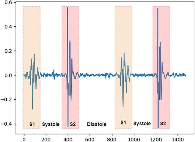
Example of a heart sound signal.
Many scholars have focused on the four-stage automatic segmentation of heart sounds. In 2010, Schmidt et al.7proposed a duration-dependent hidden Markov model (DD-HMM) for heart sound segmentation that identifies the sequence of heart sounds by explicitly modeling the duration of states. In 2015, Springer et al.8 made further improvements by using a hidden semi-Markov model (HSMM) to segment noisy heart sound recordings and improve the segmentation performance through the Viterbi algorithm. In 2019, Wei et al.9 proposed a segmentation method for heart sounds that generates envelopes from a short-time Fourier transform (STFT), in which the positions of the first and second heart sounds are determined according to different energy standard deviations in different frequency bands. In 2019, Renna10 and his team were inspired by image segmentation algorithms and proposed a heart sound segmentation method based on deep convolutional neural networks (CNNs). They combined the CNN model with a sequential time modeling process to achieve better results in heart sound segmentation.
However, the difficulty of heart sound classification based on segmented signals is how to accurately segment the four stages of heart sound signals. Heart sound signals are different due to age, sex, physical conditions and other factors. In addition, there may be differences in the location, cause and degree of heart disease, so it is even more difficult to accurately partition the heart sound signals of patients. The inaccuracy of the four-stage segmentation of heart sounds greatly affects the feature extraction effect.
To avoid the problem of heart sound segmentation, many scholars take the whole heart sound signal as input and do not distinguish between different stages of heart sounds. Aiming at the nonstationary and nonlinear characteristics of heart sound signals, Liu et al.11 proposed a support vector machine (SVM) method for classifying and recognizing heart sounds. In this method, adaptive noise complete empirical mode decomposition (CEEMDAN) permutation entropy was used as the feature vector of heart sound signals. Morteza Zabihi12 extracted effective time domain, frequency domain, and time-frequency domain features without segmentation and classified signals based on a novel neural network. Yuenyong et al.13 used a discrete wavelet transform and principal component analysis to extract features, in which the cycle length was calculated using the information in the envelope of the autocorrelation function, and finally, the features were sent to the neural network for classification. Han et al.14 calculated the subband coefficients of the cardiac signal from the extracted subband envelopes, fused autocorrelation features and used diffusion maps to unify the feature representation. Finally, they used a support vector machine (SVM) for heart sound classification. Fan Qingling et al.15 proposed a heart sound classification algorithm based on FrFT-Bark domain feature extraction and a CNN residual shrinkage network. First, they extracted the time-frequency features of the Bark-domain fractional Fourier transform from heart sound signals. Then, they introduced the deep residual shrinkage network into the convolutional neural network to construct a new classification model.
Classification methods based on whole signals are relatively simple, run faster, and are decoupled from heart sound segmentation. Therefore, these methods can better exploit the global information in heart sound signals and avoid the impact of inaccurate segmentation on classification performance. However, at present, the process of extracting these global features is relatively simple, and the extraction of information, which is usually information from the time domain, frequency domain, or time-frequency domain, is inadequate. This approach results in poor classification results, and the classification performance of these algorithms is lower than that of algorithms based on signal segmentation. We believe that heart sound signals must be studied in the statistical domain and therefore propose a higher-dimensional feature vector, which includes the time domain, frequency domain, time-frequency domain, and statistical domain features of heart sound signals, for classification tasks.
Although some of the above methods use deep networks, their high performance in the classification field has not been fully utilized. Considering that deep networks are currently focused on image recognition in the field of classification, we believe that the deep recognition networks can be used to classify heart sounds better if the multi-dimensional features of heart sounds are represented graphically.
Some researchers have attempted to convert heart sound signals into images. The first step is to extract features from a one-dimensional heart sound signal. Then, these extracted features must be transformed into the form of a matrix16. Some methods directly reshape the features to obtain a two-dimensional matrix17. The matrix obtained in this way has a strong relationship with the order of the features and ignores the correlation between the features. Alok Sharma et al.18 considered this problem and developed a new method for visualizing features of genetic data, which makes features with greater similarity closer in relative position after visualization. They developed a method for finding the corresponding position of each feature in the Cartesian coordinate system and filling the position with the feature value. In their method, PCA is used to eliminate the correlation between the feature input order and projection results. It can intuitively reflect feature correlation through the density of the point distribution in the image. At the same time, the difference in image gray level also reflects the size of the feature values, which enhances the interpretability of the image to a certain extent. The flowchart of this method is shown in Fig. 2.
Fig. 2.

Flowchart of DeepInsight18. Copyright 2019,Alok Sharma.
The DeepInsight method18 inspired us, so we proposed a cardiac audio classification method based on image expression of multidimensional features (CACIEMDF). Although the DeepInsight method can transform one-dimensional data features into two-dimensional images, there are only some discrete points with different gray levels in the obtained image, which is very different from images processed by conventional deep networks. Considering the influence of feature stacking, our CACIEMDF uses feature value summation and Gaussian mapping to fill the image pixels, retaining the spatial interaction between feature values that are closely distributed. At the same time, CACIEMDF fills the three channels of the image in different ways for the color image expression of multidimensional features. Our method exploits the powerful processing ability of the current deep network for color images to improve the classification performance.
Results
Experimental setup
Two different classification networks are used in the classification experiment of this subject, namely, the improved AOTC network and the pretrained ResNet50. The improved AOCT convolutional neural network has a unique and efficient network structure, and its core part includes four convolutional blocks. Each convolution block consists of a convolution layer, a batch normalization layer, an activation function layer and a maximum pooling layer. The maximum pooling layer in the fourth convolutional block is replaced with a fully connected layer and softmax layer to output the final classification result. This network structure optimizes the process of feature extraction, not only improves the efficiency and accuracy of feature extraction but also ensures the efficient execution of feature recognition and classification tasks and ensures the high energy efficiency of the calculation process. The AOTC network structure is shown in Fig. 3.
Fig. 3.

Diagram of the improved AOCT network.
ResNet50 selects the network model pretrained on ImageNet.
Both methods were trained through 150 rounds of iterations. Adam is selected as the optimizer, the batch size is set to 64, the initial learning rate is set to 0.0001, and the attenuation is the original 0.9 per 10 rounds.
To objectively evaluate the performance of the model, the following five indices were selected: accuracy, sensitivity, specificity, AUC and F1 score. The accuracy rate represents the ratio of the number of samples correctly predicted by the model to the total number of samples. The sensitivity represents the proportion of samples that are actually positive and are judged to be positive; the specificity represents the proportion of samples that are actually negative and are judged to be negative; and the AUC represents the area under the ROC curve and is used to describe the relationship between the sensitivity and specificity. Its value range is [0,1]. The closer it is to 1, the better the performance of the classifier. The F1 score is used to measure the accuracy of the classification model, accounting for the accuracy and recall rate of the model. The value range is [0,1]. The larger the value is, the better the performance of the model.
Comparison and classification performance
The experimental results of different image expression methods and classification networks are shown in Table 1, and the corresponding confusion matrix is shown in Fig. 4.
Table 1.
Results based on different image expression methods and combinations of classification networks with 102-dimensional feature vectors.
| Image expression method | Classification network | Acc (%) | Sen (%) | Spe (%) | AUC (%) | F1 (%) |
|---|---|---|---|---|---|---|
| Second-order | AOCT20 | 91.44 | 93.80 | 88.86 | 91.33 | 91.37 |
| Spectrum19 | Resnet50 | 93.28 | 95.77 | 90.62 | 93.20 | 93.24 |
| DeepInsight | AOCT | 91.50 | 94.08 | 88.86 | 91.47 | 91.51 |
| Resnet50 | 93.57 | 92.11 | 95.01 | 93.56 | 93.53 | |
| DeepInsight + SE | AOCT | 91.80 | 92.96 | 90.62 | 91.79 | 91.81 |
| Resnet50 | 94.14 | 94.37 | 93.84 | 94.10 | 94.11 | |
| DeepInsight + SE + CR | AOCT | 93.38 | 92.68 | 94.13 | 93.41 | 93.39 |
| Resnet50 | 94.42 | 94.37 | 94.43 | 94.40 | 94.40 | |
| DeepInsight + SE + CR + CE (CACIEMDF) | AOCT | 94.70 | 93.52 | 95.89 | 94.71 | 94.68 |
| Resnet50 | 95.68 | 96.06 | 94.43 | 95.24 | 95.26 |
Significant values are in bold.
Fig. 4.

Confusion matrix for the classification experiments.(a1) A_S. (a2) A_D. (a3) A_D_SE. (a4) A_D_SE_CR. (a5) A_C. (b1) R_S. (b2) R_D. (b3) R_D_SE. (b4) R_D_SE_CR. (b5) R_C.
The second-order spectrum method refers to the image expression method used by a laboratory at Fudan University19. DeepInsight is the method proposed by Alok Sharma18. SE refers to the stacking effect of close features, CE refers to the continuous expression of feature projection using Gaussian expansion, and CR refers to the color expression of projected images. The specific design is described in detail in the “Color image expression based on multidimensional feature vector projection” section of this paper. The data in the Table 1 show that the CACIEMDF proposed in this paper achieved the highest accuracy rate in the binary classification task of heart sounds based on image expression.
In the Fig. 4, the first behavior is a confusion matrix for classification using an improved AOCT network. The A in the title stands for AOCT, S stands for spectrum, D stands for DeepInsight, SE and CR have the same meanings as before, and C stands for the CACIEMDF proposed in this paper. The second behavior is a confusion matrix classified by ResNet50, where the R in the title stands for ResNet50 and the remaining letters have the same meaning as before.
Table 2 shows that from the perspective of the classification network, ResNet50 outperforms the improved AOTC. To analyze the effectiveness of the method more objectively, we use ResNet50 combined with 5-fold cross-validation to verify the imaging method. The number of iterations is 20, and the experimental results are shown in Table 2.
Table 2.
Results of ResNet50 combined with 5-fold cross-validation.
| Image expression method | Acc (%) | Sen | Spe | AUC | F1 |
|---|---|---|---|---|---|
| Second-order spectrum19 | 90.45 | 90.62 | 90.27 | 90.44 | 90.45 |
| DeepInsight | 89.37 | 92.30 | 86.28 | 89.29 | 89.35 |
| DeepInsight + SE | 91.59 | 94.82 | 88.20 | 91.51 | 91.58 |
| DeepInsight + SE + CR | 92.46 | 91.46 | 93.51 | 92.48 | 92.46 |
| DeepInsight + SE + CR + CE (CACIEMDF) | 92.96 | 92.16 | 93.81 | 92.98 | 92.96 |
Significant values are in bold.
As shown in Table 2, our method still achieved the highest classification accuracy, specificity, AUC and F1 scores when ResNet50 was combined with 5-fold cross-validation.The validity of the feature vector designed in this paper is also verified by the following experiments.
In the process of feature vector design, in addition to using the time domain and frequency domain features commonly used in the heart sound classification field, this paper also adds several statistical domain features, such as high-order cumulants (), first-order difference absolute sums and aggregate statistical features of autocorrelation coefficients from the 1st to 4th order (). The specific feature vector design is introduced in detail in the “Multidimensional feature extraction” section of this paper. To analyze the effectiveness of the features of the above three domains for heart sound classification, we use a random forest, LSTM and a transformer to conduct the following experiments on different feature combinations.
The experimental results of the random forest model for different feature combinations are shown in Table 3.
Table 3.
Results of random forest based on different feature combinations.
| Features | Acc (%) | Sen (%) | Spe | AUC | F1 |
|---|---|---|---|---|---|
| Time domain | 85.92 | 88.45 | 83.28 | 85.87 | 85.91 |
| Frequency domain | 91.24 | 90.14 | 92.38 | 91.26 | 91.24 |
| Statistical domain | 74.71 | 81.69 | 67.45 | 74.57 | 74.57 |
| Time-frequency–Statistical domain | 92.24 | 90.70 | 93.84 | 92.27 | 92.24 |
Significant values are in bold.
The experimental results of LSTM for different feature combinations are shown in Table 4.
Table 4.
Results of LSTM based on different feature combinations.
| Features | Acc (%) | Sen (%) | Spe | AUC | F1 |
|---|---|---|---|---|---|
| Time domain | 64.96 | 64.79 | 65.10 | 64.95 | 64.95 |
| Frequency domain | 79.91 | 82.54 | 77.13 | 79.83 | 79.87 |
| Statistical domain | 61.59 | 90.42 | 31.67 | 61.05 | 57.93 |
| Time-frequency–Statistical domain | 80.32 | 85.35 | 75.07 | 80.21 | 80.25 |
Significant values are in bold.
The experimental results of the transformer for different feature combinations are shown in Table 5.
Table 5.
Results of the transformer based on different feature combinations.
| Features | Acc(%) | Sen(%) | Spe | AUC | F1 |
|---|---|---|---|---|---|
| Time domain | 86.57 | 88.45 | 84.75 | 86.60 | 86.63 |
| Frequency domain | 94.58 | 93.24 | 95.89 | 94.57 | 94.54 |
| Statistical domain | 68.71 | 80.00 | 56.89 | 68.45 | 68.23 |
| Time-frequency–Statistical domain | 95.27 | 94.93 | 95.60 | 95.27 | 95.26 |
Significant values are in bold.
The above three tables show that the features of the time domain, frequency domain and statistical domain are all effective for the classification of heart sounds, and the features of the three domains are integrated to achieve the highest classification accuracy, AUC and F1 score.
As many current nonimage expression heart sound classification algorithms have been tested on the 2016 PhysioNet/CinC Challenge dataset21, this paper also conducts experiments on this dataset alone and compares the performance of our algorithm with that of other algorithms, as shown in Table 6.
Table 6.
Classification results obtained on the 2016 PhysioNet/CinC Challenge dataset.
| Algorithm | Acc (%) | Sen | Spe | AUC | F1 |
|---|---|---|---|---|---|
| Nassralla M | 92.0022 | 78.00 | 98.00 | / | / |
| Cheng X | 96.1623 | 93.64 | 98.67 | / | / |
| Dominguez–Morales J P | 97.0524 | 93.20 | 95.12 | / | / |
| Sinam A S | 97.8225 | 95.04 | 98.72 | / | / |
| CACIEMDF | 97.87 | 93.53 | 98.99 | 96.26 | 97.86 |
Significant values are in bold.
The experimental results of the other methods mentioned above are directly based on the data provided in their papers.
Our method was also tested on the Yaseen for multi-class (five-class) classification of heart sounds, as shown in Table 7. The training, validation, and test sets were divided in a ratio of 8:1:1, and the other experimental conditions and parameters were the same as those in the previous binary classification experiment.The experimental results are shown in Table 7.
Table 7.
Classification results obtained on the Yaseen dataset.
| Algorithm | Acc (%) |
|---|---|
| SVM | 68.00 |
| Random forest | 78.00 |
| FCN | 58.33 |
| RNN | 62.67 |
| LSTM | 57.38 |
| CNN | 79.77 |
| Transformer | 88.98 |
| CACIEMDF | 94.53 |
Since Yassen has a small amount of data, we cross-validate the model to prevent overfitting. It can be observed from the experimental results that our method still has good performance in the multi-classification task.
Discussion
The experiments in this paper are based on public datasets and their labels. The abnormalities of cardiac audio are varied. Some of the datasets used more detailed pathological features, such as aortic stenosis, mitral stenosis, mitral regurgitation and mitral valve prolapse. It is unclear what further classification information exists, for example, tachycardia.
According to the current dataset, the tachycardia audio belongs to the category of normal audio, but when we design feature vectors and classify them, the tachycardia audio is classified as abnormal by the network. The decrease in classification accuracy caused by this classification error should be considered. Visualization images of normal audio and tachycardia audio are shown in Fig. 5.
Fig. 5.

Visualization of normal heart sound data and tachycardia heart sound data. (a) Normal heart sounds. (b) Tachycardia heart sounds
In 2020, M D et al. proposed a heart sound classification method based on MFCCs + CRNN26, and the classification accuracy of this method reached 98.34%. However, because the detailed information of its network was not disclosed, the text description and network structure diagram in the article are inconsistent, and the author does not provide relevant codes or explanations. Based on the author’s understanding of the algorithm described in this article, the data preprocessing, feature extraction, and network building parts were reproduced. However, the accuracy of the classification experiment conducted afterward was much lower than that of the algorithm described in this article. In addition, the focus of this paper is on the color image representation of audio data, so MFCCs + CRNN are not included in the comparison algorithms in this paper.
The main contributions of this work are as follows:
The existing methods for extracting heart sound signal features are not comprehensive, and the statistical domain features are more sensitive to small changes in signals, which is more suitable for nonstationary medical signals such as heart sound signals. Therefore, a 102-dimensional feature vector integrating the information of the time domain, frequency domain and statistical domain is designed to comprehensively interpret and express heart sound signals.
Most heart sound classification methods focus on the analysis and research of relevant features of one-dimensional heart sound signals, while most deep learning methods have better generalization performance and feature interpretation ability in two-dimensional image space, for transferring the good performance of the deep network to the audio classification task, we expressed the heart sound signal graphically.
The feature differentiation ability and image richness of traditional heart sound signal pictorial expression methods are limited. We mined the potential information of features and optimized the representation form of features to enhance the information density of feature images and enrich the content of feature images.
The method proposed in this paper, while successful in converting multidimensional features of cardiac audio into image representations, facilitates the use of the classification performance of deep networks. Inevitably, some features overlap in the generated image results, resulting in information confusion, and the image is sparse, which will also have a certain impact on the classification performance of the network. This method is designed for binary classification of heart sounds. Considering that abnormal heart sounds can be further classified, the projection space filling method needs to be designed when multiple classification tasks are carried out.
Methods
The following will provide a detailed introduction to the CACIEMDF algorithm framework that we have developed. Prior to delving into the algorithm, we will first present the data set’s source, the relevant preprocessing operations conducted on it, and the 102-dimensional feature vector that we have designed. Subsequently, three specific enhancements of our algorithm framework will be introduced.
Datasets
We collected heart sound data from Yaseen201827 (Database1), the 2016 PhysioNet/CinC Challenge21 (Database2), and the 2011 PAsCAL challenge dataset (Database3). The types and quantities of audio in each dataset are shown in Tables 8, 9 and 10.
Table 8.
Database1.
| Folder | Heart sound state | Number |
|---|---|---|
| N | Normal | 200 |
| AS | Aortic stenosis | 200 |
| MS | Mitral stenosis | 200 |
| MR | Mitral regurgitation | 200 |
| MVP | Mitral valve prolapse | 200 |
Table 9.
Database2.
| Folder | Pathological feature | Normal | Abnormal |
|---|---|---|---|
| a | MVP | 292 | 117 |
| b | Murmurs (noise) | 104 | 386 |
| c | MR, AS | 24 | 7 |
| d | None | 28 | 27 |
| e | Murmurs | 183 | 1958 |
| f | None | 34 | 80 |
Table 10.
Database3.
| Folder | Number of normal | Number of abnormal | Number of additional | Number of artificial |
|---|---|---|---|---|
| A | 31 | 34 | 19 | 40 |
| B | 320 | 95 | 46 | 195 |
Yaseen201827 provided a dataset, Database1, which contains heart sound data that can be divided into normal and abnormal data. The data were further subdivided into five categories, including one normal (N) category and four abnormal categories: aortic stenosis (AS), mitral stenosis (MS), mitral regurgitation (MR), and mitral valve prolapse (MVP). Detailed audio types and quantities are shown in Table 8.
The Database2 dataset used in the 2016 PhysioNet/CinC Challenge21 was composed of 6 different databases (a–f) with a total of 3240 heart sound recordings, of which 665 were normal and 2575 were abnormal. The duration of these recordings varied, with the shortest being 5 s and the longest being over 120 s. The heart sounds recorded in the dataset from healthy subjects were all labeled normal, and those from patients with confirmed heart disease were labeled abnormal. Most of these patients have a variety of heart diseases, especially heart valve defects and coronary artery disease. These abnormal heart sounds were recorded without further information on disease categories. All the recordings in the dataset were resampled to 2000 Hz, as shown in Table 9, for specific audio types and quantities.
The data in the 2011 PASCAL Challenge dataset, Database3, come from two different sources: (A) data collected from the public via the iStethoscope Pro iPhone app and (B) data from clinical trials in hospitals using DigiScope, a digital stethoscope, where some of the audio contains excessive noise. Table 10 lists the audio types and quantities.
We selected all audio from Database1 and Database2, as well as the normal and abnormal audio from Database3, as our experimental dataset. Among them, there are 3504 abnormal audio recordings, with the longest duration being 101.67 s and the shortest duration being 0.85 s. The number of normal audio recordings is 1216, with the longest duration being 121.99 s and the shortest duration being 0.76 s.
Data preprocessing
Considering the problems of balancing positive and negative samples and that the periodicity of normal heart sounds is obvious, we split normal audio that lasts longer than 10 s into equal segments as new samples. In this way, it can be ensured that the audio segment still contains enough complete heart sound cycles, thus retaining the characteristic information of normal audio when the sample duration is increased. After splitting, there are 3452 normal audio recordings, which is close to the number of abnormal samples, achieving data equalization. The total number of normal and abnormal samples reached 6956.
In our experiment, the positive and negative samples were divided into a training set, verification set and test set at a ratio of 8:1:1.
Due to differences in the audio collection settings, equipment, noise and other factors among the three datasets, there are significant differences in the audio amplitude. Therefore, before extracting features from the audio, the data are denoised, downsampled and normalized. The flow chart is shown in Fig. 6.
Fig. 6.

Flow chart of data preprocessing.
In addition to the obvious periodic peaks, some recordings also contain some unusually sharp peaks, as shown in Fig. 7. By measuring the amplitude of the sample relative to the standard deviation, we find that the sample with the sharp peak has a ratio as high as 94, but the average ratio of all the samples is 10. This means that sharp spikes are rare, and we think that this rare occurrence is caused by noise, not a heart murmur.
Fig. 7.
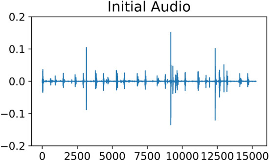
Visualization of audio with sharp noise peaks.
To remove the influence of these outliers, we calculated the divergences of the audio amplitude extremes. The calculation is as follows:
| 1 |
where represents the number of audio recordings, represents the mean value of the amplitude of the sampling points and represents the standard deviation of the amplitude of the sampling points. According to the statistics, the mean value of is close to 10. Based on this, we calculate the upper and lower bounds of the audio amplitude according to the following formula:
| 2 |
| 3 |
For the amplitude values within the boundary in the audio, no changes are made. The amplitude values outside the boundary are set to the boundary value.
| 4 |
The amplitude of the processed audio sampling points is shown in Fig. 8.
Fig. 8.
Visualization of audio after outlier removal.
A comparison of Figs. 7 and 8 shows that there are obvious outliers in the original amplitude plot of the sampling points, whose maximum value can reach 0.15. After denoising with the upper and lower bounds, the overall amplitude is [− 0.1, 0.1], which reduces the influence of extreme values to a certain extent.
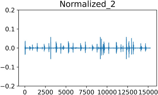
The upper and lower bounds of the amplitude vary slightly for each sample. To avoid the influence of the amplitude range on the feature extraction process, we use the following formula to scale the overall amplitude range to [− 1,1].
| 5 |
where is the sequence of sampling points of the th sample and is the th sampling point of the th sample. represents the absolute value, and is the scaled sequence of sampling points, as shown in Fig. 9.
Fig. 9.

Visualization of the normalized audio.
Multidimensional feature extraction
Feature extraction is a key step in the diagnosis and recognition of heart sound signals. Since heart sound is a time-dependent signal, its kurtosis28,29, skewness28,29, mean energy30,31, short-time zero crossing rate32,33 and other time domain features are widely used. Frequency domain features have stronger discriminatory ability than time domain features34, and the feasibility of identifying changes or patterns in heart sound signals is greater. The spectral information of a single frequency can be used, and the spectral information of a frequency band can also be used to help distinguish different types of heart sound signals.
In this paper, in addition to those of the time domain and frequency domain, the characteristics of the statistical domain can also be used to describe heart sound signals. We added the statistical features of higher-order cumulants, first-order difference absolute sums, and first-fourth order autocorrelation coefficients to enrich the multidimensional feature vectors of heart sounds. In summary, we designed a 102-dimensional feature vector that contains time domain (), frequency domain (), and statistical domain () features of heart sound signals. The specific meanings are shown in Table 11.
Table 11.
Extracted features and their meanings.
| Features | Meanings |
|---|---|
| Kurtosis, skewness | |
| Maximum, minimum, mean and variance of the amplitude envelope | |
| Mean energy, short-time zero crossing rate | |
| 10th-order linear predictive cepstral coefficients | |
| Information entropy, Tsallis entropy | |
| Entropy and variance of the spectrum | |
| MFCC features | |
| MFCC-based features | |
| Wavelet-based features | |
| Power spectral density-based features | |
| High-order cumulants (1st to 4th) | |
| First-order difference absolute sum | |
| Aggregated statistical features of the autocorrelation coefficients of each order (1st to 4th) | |
| Mean, variance, entropy, energy, skewness and kurtosis of the energy spectrum | |
| Mean and standard deviation of spectral peaks | |
| LFCC features | |
| FBank features |
The MFCC frequency cepstrum coefficient (MFCC) is widely used in speech recognition, and its extraction process includes several key steps, such as preprocessing, fast Fourier transform (FFT), Mel filter bank (Mel), logarithm operation, discrete cosine transform (DCT), and dynamic feature extraction. The MFCC can effectively represent the characteristics of speech signals combined with human hearing characteristics and achieve remarkable results in automatic speech and speaker recognition. The characteristics are calculated based on the MFCC35 as follows:
| 6 |
| 7 |
| 8 |
where represents the th MFCC of the th frame and , , and represent the minimum value, maximum value and skewness, respectively. represents the mean value, . represents the set of MFCC features.
The wavelet transform is often used to extract the features of heart sound signals. On the one hand, it can perform time-frequency analysis of heart sound signals, providing greater analysis precision and accuracy than a traditional Fourier transform; on the other hand, the signal can be analyzed at different scales to capture the details and global characteristics of the signal. Based on the characteristics of the wavelet transform35, Daubechies 4 should be used to calculate the heart sound signal first. The formulas are as follows:
| 9 |
| 10 |
| 11 |
| 12 |
The discrete wavelet transform (Daubechies 4) is applied to the heart sound signal, where represents the 5th order approximation coefficient. , , and represent the detail coefficients of the 3rd, 4th, and 5th orders, respectively. denotes the variance, is the Rayleigh entropy with , is the Shannon entropy, and represents the th coefficient in the sequence of coefficients.
The power spectral density is an important physical quantity that characterizes the power distribution of a signal in the frequency domain. It reflects the power carried by a signal at a unit frequency and is the energy representation of a signal in the frequency domain. It is very important for the analysis and recognition of signal characteristics, and its calculation needs to first perform a Fourier transformation on the signal and then take the square of the module. The calculation formula based on the characteristics of power spectral density35 is shown as follows:
| 13 |
| 14 |
| 15 |
where represents the power spectral density, is the modified power spectral density centroid, and and represent the areas under the AUC curve within two specified frequency intervals.
In addition to the time-domain and frequency-domain features described above, this paper also introduces the characteristics of the statistical domain. The higher-order cumulant is the coefficient of the Taylor series expansion of the second characteristic function, which can provide more information than traditional second-order statistics. Moreover, it has strong robustness to Gaussian noise, so it can extract signal features effectively in the presence of noise interference and is especially useful for analyzing and processing non-Gaussian signals. The specific calculation process is as follows:
The characteristic function of the random variable can be written in the form of the Laplacian operator:
| 16 |
Taking the th derivative of the characteristic function, we obtain
| 17 |
The value at the origin is equal to the th moment of
| 18 |
is often referred to as the moment-generating function of , also known as the first characteristic function.
is known as the cumulant-generating function of , also called the second characteristic function. The th cumulant of a random variable is defined as the value of its th derivative at the origin of its cumulant-generating function .
| 19 |
Since , and . Setting , we obtain and .
The first and second cumulants can be obtained36,37.
| 20 |
| 21 |
The third and fourth cumulants can be obtained in a similar manner36.
| 22 |
| 23 |
The absolute sum of first-order differences is a method used for feature extraction in the analysis of time-series data. It calculates the absolute values of the difference between two consecutive adjacent data items in the time-series data and accumulates these absolute values to obtain a total amount. The specific calculation is as follows:
| 24 |
In the analysis of time-series data, the autocorrelation coefficient is a statistical index used to measure the correlation between data values of the same time series at different time points, which provides information about the correlation degree of time series in different lag periods and further reveals the inherent law of time series. This paper extracts the aggregated statistical characteristics of the autocorrelation coefficients of each lag period, and the specific calculation formula is as follows:
| 25 |
where is the mean value and takes values of 1, 2, 3, and 4 as , , , and , respectively.
To display the distribution of 102-dimensional features more directly, we use t-distributed stochastic neighbor embedding (t-SNE) to visualize multidimensional feature vectors. First, all samples (including normal and abnormal samples) are input into the feature extraction module to obtain the multidimensional feature data of the samples. Then t-SNE is used to generate the feature distribution diagram of the low-dimensional space, as shown in Fig. 10, where black represents negative samples and red represents positive samples.
Fig. 10.

Distribution of 102-dimensional features.
The Fig. 10 shows that the 102-dimensional features we extracted have a very clear feature interface, and the point clusters of the two colors are relatively concentrated (the negative samples have different categories of heart sound abnormalities, so the black point clusters are divided into several parts). This shows that the features we extracted are highly correlated with the categories and have high discriminability in positive and negative samples, which is conducive to the correct division of positive and negative samples by the network. Other relevant experimental results are shown in Tables 3, 4 and 5
In order to understand the importance of different features,we divided 102-dimensional features into five groups of Fbank features, LFCC features, MFCC features, autocorrelation features and other features. The parentheses after the feature set indicate the range of the feature. We used random forests to assess the importance of these five sets of features and drew an importance pie chart, as shown in the Fig. 11.
Fig. 11.
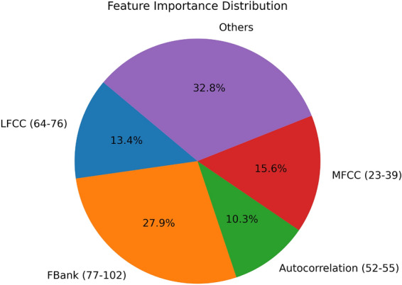
importance assessment of 102-dimensional features.
In assessing the importance of 102-dimensional characteristics of species, we found that the 86th and 87th features (Fbank features), the 70th feature (LFCC features), the 1st feature (kurtosis), and the 58th feature (entropy of energy spectrum), etc., rank among the top in the importance assessment.This suggests that these features are important in the task of classifying heart sounds.
In order to analyze the interpretability of these important features, we selected the three most important features from the 102-dimensional features extracted from Yaseen dataset for numerical statistics, and the results were shown in Table 12. The Fbank feature simulates the law of sound received by the ear and pays more attention to the low frequency part of the heart sound signal, while the LFCC feature can better characterize the high frequency information of the signal through a linear filter. Since normal heart sound signals are low frequency signals, while heart murmurs often contain a large number of high frequency signals, the Fbank and LFCC features of normal samples are significantly smaller than those of abnormal samples. Kurtosis represents the steepness of signal peak and also reflects the speed of signal change. AS is a heart murmur caused by aortic stenosis, the aortic valve cannot fully open during systole, resulting in high-frequency noise when blood flows through the narrowed valve, which slows down the signal change between S1-systole-S2. Therefore, the kurtosis of AS is significantly smaller than that of other categories.
Table 12.
Numerical statistics of some important features on the Yaseen.
| Category | Fbank (86) | LFCC (70) | Kurtosis |
|---|---|---|---|
| N (Normal) | 0.015 | − 78.989 | 13.234 |
| AS (Aortic Stenosis) | 0.591 | − 36.429 | 6.946 |
| MR (Mitral regurgitation) | 0.511 | − 38.429 | 12.789 |
| MS (Mitral stenosis) | 0.152 | − 46.238 | 14.957 |
| MVP (Mitral valve prolapse) | 0.183 | − 44.600 | 14.682 |
The above important features are closely related to the pathology of heart sound signals, and the effectiveness of the extracted features can also be preliminarily demonstrated through importance assessment experiments.In the future, we will further study the pathologic interpretability of heart sound features.
Color image expression based on multidimensional feature vector projection
We propose a color image expression method (CACIEMDF) based on multidimensional feature vector projection. Our method first uses PCA reduction and convex hull algorithms to project the above 102-dimensional feature vector into a 2-D image coordinate system and finds the corresponding coordinate representation for each feature component. The feature values projected to the same pixel position are summed. Then, the color image representation of the heart sound signal is obtained by filling three channels of the color image with the value of the one-dimensional feature component and its divergences to the two categories. Finally, the Gaussian model is used to render the image to enrich the image content so that the image content is not only discrete points. The flowchart is shown in Fig. 12.
Fig. 12.

Flowchart of the CACIEMDF.
Stacking effect of close-range features
The construction of the projection space first represents the expanded sample feature set as a matrix with 102 (feature dimension) rows and 6956 (sample quantity) columns. PCA dimensionality reduction is used to transform the feature data into a matrix with 102 rows and 2 columns, representing the relative positions of 102 features. Then, the convex hull algorithm is used to find the smallest rectangle that can cover all feature points. By rotating it, a Cartesian coordinate system and the position coordinates of each feature in the coordinate system are obtained. Each feature can be mapped to a grayscale image through a pair of 2D coordinate representations.
The two-dimensional data obtained by PCA dimensionality reduction are not affected by the feature input order. Therefore, assuming that the feature content is certain and the input order is changed, the dimensionality reduction data obtained are the same; that is, the obtained feature coordinate array representations are consistent. In this case, the coordinate system and position obtained by the convex hull algorithm are also fixed. Unlike the simple arrangement of input features into a two-dimensional array, it will be affected by the input order of the features. The diagram is shown in Fig. 13.
Fig. 13.

Schematic diagram of the different filling methods. (a) Sequential filling. (b) Reverse filling.(c) PCA combined with the convex hull algorithm.
Two or more feature positions may be the same when calculating the coordinate representation of the feature vector component. DeepInsight [18] took the average of multiple feature values to fill in this pixel. If the positions of some features in the projection space are close enough to be represented by the same pixel coordinates, we believe that these features can be stacked during image expression to achieve feature fusion. The results are shown in Fig. 14.
Fig. 14.

Stacking effect of close-range features. (a) Fill results without the stacking effect. (b) Fill results with the stacking effect. (c) 3D grayscale distribution of (a). (d) 3D grayscale distribution of (b)
In Fig. 14a,b, feature images generated by filling the corresponding pixels with feature values are shown. Most of the images have black background areas, which are positions without feature filling, and only a small number of pixels are filled with feature values, which are displayed as highlights of different gray levels on the feature image. The readability of feature images is limited by the number of features and grayscale, so we show the corresponding three-dimensional grayscale distribution in Fig. 14c,d to help show the grayscale distribution in feature images.
A comparison of the gray distributions at three positions (1, 2, and 3) is shown in Fig. 14c,d. Adding the values of multiple feature components represented by the same coordinate using the stacking effect can make the coordinate positions representing multiple feature components more prominent, and their gray values are larger and visually more significant.
Color representation of the projected image
The images in Fig. 14 are gray images, whereas existing deep learning networks have high performance in color image classification. Our CACIEMDF projects the feature vector into a three-channel projection space to obtain the color image expression, which can exploit the recognition ability of deep networks. The value of the 1D feature component and its divergences to the two categories are used to fill the three channels. Our method calculates the mean and variance of each feature component of the positive and negative samples, respectively, and then calculates the degree of dispersion as follows.
| 26 |
| 27 |
| 28 |
In , is taken as r,g,and b to represent three different channels, indicates that the image coordinate position of the th feature projection is , represents the feature value of the th feature, represents the mean of the feature values of the th feature in all normal samples, and represents the standard deviation of the feature values of the th feature in all normal samples. Similarly, represents the mean of the feature values of the th feature in all abnormal samples, and represents the standard deviation of the feature values of the th feature in all abnormal samples. The color representation of Fig. 14b is shown in Fig. 15.
Fig. 15.

Color representation of projected images.
Comparing Figs. 15 and 14b shows that the color expression of the feature image can be realized by filling the three channels of the feature image differentiated by the category dispersion of the designed features. The feature filling pixels in the Fig. 15 above are shown in blue and red. Different samples have different feature dispersions, and the colors displayed by the feature points will also be different.
Considering that RGB images have only three channels, the above filling method is not suitable for multi-classification tasks. In multi-classification tasks, our approach requires some changes. First, the mean and standard deviation of the eigenvalues of the samples of each class are calculated, and then reduced to two dimensions using PCA. The rest of the process is consistent with the filling method of the binary classification, as shown in Equations 29 to 31.
| 29 |
| 30 |
| 31 |
The feature mean value of the five categories is represented as , and the standard deviation is represented as . PCA dimensionality reduction method is used for the mean value and standard deviation sets respectively to obtain and . Through the above method, we can realize the color image representation method of any category.
Continuous expression of the feature projection realized by using the Gaussian extension method
Although Fig. 15 shows the color expression, the image still contains discrete points, making it quite different from the natural image. Therefore, our method uses Gaussian kernel mapping to project the features into the image and superimpose them so that the distribution of features in the image will no longer be discrete points. The continuous expression of Fig. 15 is shown in Fig. 16.
Fig. 16.

Continuous expression of feature projection.
From the above figure, the use of Gaussian extension can make the content of the image more continuous.
Author contributions
J.H. implemented the design of the overall scheme, J.R. conducted the experimental verification and algorithm testing, S.L. conducted the algorithm design and part of the experiments, W.C. provides ideas for the innovation of this paper, Y.O. and J.H. conducted the analysis of the results. All authors reviewed the manuscript.
Data availibility
Yaseen2018 data is available from https://github.com/yaseen21khan/Classification-of-Heart-Sound-Signal-Using-Multiple-Features-. 2016 PhysioNet/CinC Challenge data is available from https://physionet.org/content/challenge-2016/1.0.0/#files. 2011 PAsCAL challenge data is available from http://www.peterjbentley.com/heartchallenge/.
Footnotes
Publisher’s note
Springer Nature remains neutral with regard to jurisdictional claims in published maps and institutional affiliations.
These authors contributed equally: Hu Jing, Ren Jie and Lv Siqi.
References
- 1.Zanettin, F. World Health Statistics 2024 (2024).
- 2.Yang, H. Research on Diagnosis Methods for Heart Diseases Based on Analysis of Heart Sound Signals. Master’s thesis, Lanzhou University of Technology (2023).
- 3.Cao Li, S. Y., Zhao De’an. Heart sound diagnosis method based on artificial neural network and wavelet analysis. Microcomput. Inf. 311–312+302 (2007).
- 4.Zhimin, R. Heart Sound Signal Classification Based on Deep Learning. Master’s thesis, Jilin University (2023).
- 5.Li Zhanming, W. Z., Han Yang. Heart sound signal time-frequency analysis method research. China Med. Equipment.9, 1–4 (2012).
- 6.Liang, H., Lukkarinen, S. & Hartimo, I. Heart sound segmentation algorithm based on heart sound envelogram. IEEE (1997).
- 7.Schmidt, S. E., Holst-Hansen, C., Graff, C., Toft, E. & Struijk, J. J. Segmentation of heart sound recordings by a duration-dependent hidden Markov model. Physiol. Meas.31, 513–529 (2010). [DOI] [PubMed] [Google Scholar]
- 8.Springer, D. B., Tarassenko, L. & Clifford, G. D. Logistic regression-HSMM-based heart sound segmentation. IEEE Trans. Biomed. Eng.63, 822 (2016). [DOI] [PubMed] [Google Scholar]
- 9.Wei, W., Zhan, G., Wang, X., Zhang, P. & Yan, Y. A novel method for automatic heart murmur diagnosis using phonocardiogram. In Proceedings of the 2019 International Conference on Artificial Intelligence and Advanced Manufacturing (2019).
- 10.Renna, F., Oliveira, J. H. & Coimbra, M. T. Deep convolutional neural networks for heart sound segmentation. IEEE J. Biomed. Health Inform. 1 (2019). [DOI] [PubMed]
- 11.Liu Meijun, D. S. & Wu, Q. Research on heart sound classification method based on adaptive noise complete ensemble empirical mode decomposition permutation entropy combining with support vector machine. J. Biomed. Eng.39, 311–319 (2022). [DOI] [PMC free article] [PubMed] [Google Scholar]
- 12.Zabihi, M., Rad, A. B., Kiranyaz, S., Gabbouj, M. & Katsaggelos, A. K. Heart sound anomaly and quality detection using ensemble of neural networks without segmentation. IEEE (2017).
- 13.Yuenyong, S., Nishihara, A., Kongprawechnon, W. & Tungpimolrut, K. A framework for automatic heart sound analysis without segmentation. Biomed. Eng. Online10, 13–13 (2011). [DOI] [PMC free article] [PubMed] [Google Scholar]
- 14.Han, J.-Q. & Deng, S.-W. Towards heart sound classification without segmentation via autocorrelation feature and diffusion maps. Future Gener. Comput. Syst. FGCS.60, 13–21 (2016). [Google Scholar]
- 15.Fan Qingling, G. T., Yang, H. Heart sound classification algorithm based on frft-bark feature extraction and cnn residual shrinkage network. J. Yunnan Univ. (Nat. Sci. Ed.)45, 564–574 (2023).
- 16.Nanni, L., Brahnam, S. & Lumini, A. Texture descriptors for representing feature vectors. Expert Syst. Appl.122, 163–172 (2019). [Google Scholar]
- 17.Lu, M., Wang, Z., Gao, D. & Zhu, Y. Imat: Matrix learning machine with interpolation mapping. Electron. Lett.50, 1836–1838 (2014). [Google Scholar]
- 18.Sharma, A., Vans, E., Shigemizu, D., Boroevich, K. A. & Tsunoda, T. Deepinsight: A methodology to transform a non-image data to an image for convolution neural network architecture. Sci. Rep.9 (2019). [DOI] [PMC free article] [PubMed]
- 19.Zanettin, F. Heart sound (PCG) classification algorithm—based on deep learning—raspberry pi for auscultation of heart disease (2024).
- 20.Alqudah, A. M. Aoct-net: a convolutional network automated classification of multiclass retinal diseases using spectral-domain optical coherence tomography images. Med. Biol. Eng. Comput.58, 41–53 (2019). [DOI] [PubMed] [Google Scholar]
- 21.Clifford, G. D., Liu, C., Moody, B., Springer, D. & Mark, R. G. Classification of normal/abnormal heart sound recordings: The physionet/computing in cardiology challenge 2016. IEEE (2017).
- 22.Nassralla, M., Zein, Z. E. & Hajj, H. Classification of normal and abnormal heart sounds. In International Conference on Advances in Biomedical Engineering, 1–4 (2017).
- 23.Cheng, X., Huang, J., Li, Y. & Gui, G. Design and application of a laconic heart sound neural network. IEEE Access. (2019).
- 24.Juan, P. et al. Deep neural networks for the recognition and classification of heart murmurs using neuromorphic auditory sensors. IEEE Trans. Biomed. Circuits Syst. (2017). [DOI] [PubMed]
- 25.Sinam, A. S., Ningthoujam, D. D. & Swanirbhar, M. An improved unsegmented phonocardiogram classification using nonlinear time scattering features. Comput. J.6 (2022).
- 26.Deng, M., Meng, T., Cao, J., Wang, S. & Fan, H. Heart sound classification based on improved MFCC features and convolutional recurrent neural networks. Neural Netw.130 (2020). [DOI] [PubMed]
- 27.Yaseen, Son, G. Y. & Kwon, S. Classification of heart sound signal using multiple features. Appl. Sci.8 (2018).
- 28.Potes, C., Parvaneh, S., Rahman, A. & Conroy, B. Ensemble of feature-based and deep learning-based classifiers for detection of abnormal heart sounds. IEEE (2016).
- 29.Kay, E., Agarwal, A. Dropconnected neural networks trained on time-frequency and inter-beat features for classifying heart sounds. Physiol. Meas. (2017). [DOI] [PubMed]
- 30.Jian, W. Research on Heart Sound Energy Analysis Method and Its Application. Master’s thesis, Chongqing University (2013).
- 31.Wenru, Z. Research on Heart Sound Signal Classification Algorithm Based on Energy Entropy. Master’s thesis, Xihua University (2020).
- 32.Cui Xingxing, S. Z. A new method for feature extraction of respiratory sound signal and its application. J. Chin. Med. Phys.35, 214–218 (2018). [Google Scholar]
- 33.Zhang Tiemin, H. J. Detection of avian influenza sick chickens based on audio features and fuzzy neural network. J. Agric. Eng.35, 168–174 (2019). [Google Scholar]
- 34.Huang, J., Zheng, A., Shakeel, M. S., Yang, W. & Kang, W. Fvfsnet: Frequency-spatial coupling network for finger vein authentication. IEEE Trans. Inf. Forensics Secur.18, 1322–1334. 10.1109/TIFS.2023.3238546 (2023). [Google Scholar]
- 35.Zabihi, M., Rad, A. B., Kiranyaz, S., Gabbouj, M. & Katsaggelos, A. K. Heart sound anomaly and quality detection using ensemble of neural networks without segmentation. IEEE (2017).
- 36.Wang, Q. J. S., Le, J. Research on high-order spectral analysis technique of EEG signal. Chin. Med. Devices J.33, 79–82 (2009).
- 37.Liu Lian, L. Y. Simulation research on image discrimination method based on higher-order cumulants. Comput. Simul.28, 264–267+284 (2011).
Associated Data
This section collects any data citations, data availability statements, or supplementary materials included in this article.
Data Availability Statement
Yaseen2018 data is available from https://github.com/yaseen21khan/Classification-of-Heart-Sound-Signal-Using-Multiple-Features-. 2016 PhysioNet/CinC Challenge data is available from https://physionet.org/content/challenge-2016/1.0.0/#files. 2011 PAsCAL challenge data is available from http://www.peterjbentley.com/heartchallenge/.