Landscape ecological risk assessment and driving factor analysis in southwest china

Abstract

Landscape ecological risk assessment and ecological network construction are of great significance for optimizing territorial functions and reducing regional ecological risks. Based on the production-living-ecological space perspective, this study evaluated the spatiotemporal differentiation characteristics of landscape ecological risk and its driving mechanism in Southwest China and constructed a landscape ecological network. The results showed that the proportions of ecological space, production space and living space to the total space in 2020 were 74.35%, 24.55% and 1.10%, respectively. The industrial production space had the highest growth rate, increasing by 9.8 times from 2000 to 2020. During the study period, the average value of the ecological risk index ranged from 0.2 to 0.21 for the whole landscape. The geographical distribution of ecological risk zones showed significant differences, with risk zones showing a transition from high-risk and low-risk to medium-risk zones. A total of 105 ecological corridors and 156 ecological nodes have been constructed in the 2020 ecological network. The northeastern part of the study area needs better landscape connectivity and should be focused on ecological protection. Random Forest (RF) and Geodetector modeling showed that anthropogenic disturbance and land use levels have strong explanatory power for the evolution of ecological risk in the landscape. The interactions between anthropogenic disturbance, natural climate and regional economy are essential factors in the spatiotemporal differentiation of ecological risk. This study provides scientific references for ecological risk research and the promotion of high-quality development in Southwest China.

Introduction

With the rapidly accelerating level of global industrialization and urbanization and the rising economy, the form and function of the land that supports human activities related to the economy and society have undergone significant changes. The land use structure has gradually become unbalanced, and the sustainable use of national land space is facing enormous challenges¹. The concept of the “production-living-ecological space” (hereinafter referred to as PLEs) is a function-oriented land space management and layout optimization method proposed in response to the issues arising from the traditional single land use model². This concept holds significant theoretical and practical value as it aims to create intensive and efficient production space, livable living space, and beautiful ecological space, thereby enhancing the effectiveness of land use and supporting the sustainable development of regional areas³. A healthy landscape ecological pattern is an essential foundation for maintaining ecosystem stability, sustainable land use, and the coordination of PLEs⁴. Since the composition and layout of different landscape types can result in varying resistances to external disturbances⁵, the heterogeneity of regional landscape patterns can impact the supply of ecosystem services to humans, resulting in potential ecological risks^6,7. Therefore, it is of great significance to construct a regional landscape ecological security pattern from the perspective of function-oriented optimal layout of PLEs.

Ecological risk reflects the bearing capacity of the ecosystem to risks brought about by external disturbances^8,9. Ecological risk assessment (ERA) is the process of evaluating the likelihood of environmental impact due to exposure to one or more environmental stressors¹⁰, and it is often used to evaluate the overall level of environmental protection¹¹. Landscape patterns provide basic information about landscape type and spatial structure, which can characterize the degree of risk from comprehensive regional disturbances and evaluate the spatiotemporal heterogeneity of ecological risk under disturbances¹². Therefore, ERA based on landscape patterns has been widely used^13,14. Mansori et al¹⁵. assessed the ecological vulnerability of forest ecosystems in the Dadabad region using quantitative landscape indicators. Dadashpoor et al¹⁶. used spatial metrics and a landscape expansion index to analyze changes in landscape patterns and discovered that urbanization has led to increased fragmentation and heterogeneity in urban areas. After completing the ecological risk assessment, the spatial distribution and optimization of ecological security can be determined by constructing a landscape ecological network. Ecological networks are necessary to achieve the coupling of landscape structure and function, maintain ecosystem function, increase landscape connectivity, and reduce the negative impacts of landscape fragmentation on species survival^17,18. It is mainly composed of three ecological elements: ecological sources, ecological corridors, and ecological nodes¹⁹. Currently, the construction of ecological networks based on the minimum cumulative resistance (MCR) model has been widely applied in urban expansion boundary determination, non-point source pollution control, construction of ecological and economic zones, and protection of nature reserves, etc^20–22. However, existing studies have mainly constructed landscape ecological networks based on land use patterns, without comprehensively considering the effects of landscape fragmentation, disturbance, and other landscape factors on ecological flow diffusion. Therefore, this study will construct a landscape ecological network based on landscape ecological risk assessment to enhance landscape connectivity and improve ecological risk resistance in Southwest China.

Additionally, landscape ecological patterns often result from multiple drivers within the landscape structure¹⁶. Understanding the causes of landscape ecological risk can provide a scientific basis for the multifunctional utilization of regional ecosystems and the formulation of management policies. Thus, studying the driving factors behind the spatiotemporal evolution of regional ecological risks is worthwhile. Unlike traditional methods such as principal component analysis and geographically weighted regression^23,24 Geodetector is a statistical tool used to measure spatial stratified heterogeneity and make attributions²⁵. It is advantageous because it is not limited by linear assumption, and the number of driving variables and their linear relationships do not significantly impact the results²⁶. Therefore, it effectively explains the driving factors of spatial heterogeneity and their interactions²⁷. Additionally, the Random Forest (RF) model is a machine-learning algorithm known for its robust generalization and stable performance. It boasts superior accuracy and performance compared to traditional linear regression models and can be effectively utilized for ecological risk analysis²⁸. Understanding the impact of changes in land use/cover, climatic conditions, and economic factors on landscape ecological risks is crucial for achieving regional sustainability. Therefore, in this study, we qualitatively analyzed ecological risk drivers based on the spatial distribution patterns of ecological risk assessed by PLEs, considering land use, socio-economic activities, and natural conditions, using RF and Optimal Parameter Geodetector models. Additionally, we quantitatively analyzed the interactions among these factors using Geodetector Interaction models.

Southwest China contains the most extensive karst area in the world, situated at the intersection of the riverine and mountain front disaster zones, two of the three major disaster zones in China. The unique topography, variable climate, and rapid urbanization have led to an imbalance in land use structure, increased landscape fragmentation, and ecosystems facing multiple sources of risk²⁹. During the rapid urbanization of this karst region, assessing the ecological risk value of the landscape, exploring the driving factors of ecological risk, and effectively promoting regional land transformation and the healthy development of the ecological environment have become significant scientific challenges. Using land use data from the PLEs taxonomy, we employed multiple indicators to comprehensively evaluate ecological risks, construct an ecological network, and analyze the driving factors of ecological risk within the study area. The purpose of this study ares: (1) to analyze land cover types and land use changes of the PLEs in the urbanization process of Southwest China over the past 20 years; (2) to comprehensively evaluate the level of ecological risk, its spatial autocorrelation, and spatial aggregation distribution in the region at different periods, and to construct an ecological risk safety network; and (3) to identify the ecological risk drivers and propose development suggestions for Southwest China based on the research findings.

 Materials and methods

Study area

The study area is located in southwestern China and includes five provinces and municipalities directly under the Central Government, namely, Yunnan, Guizhou, Guangxi, Sichuan, and Chongqing (longitude 97°15’–112°11’E, latitude 21°04’–34°19’N). The total area is 13.76 × 10⁵km², accounting for 14.34% of the land area of China. The study area is high in the west and low in the east, consisting of complex landform types such as the Yunnan-Guizhou Plateau, Sichuan Basin, and Guangxi hills and mountains. The area has widely exposed carbonate rocks, making it one of the major karst regions in China. The ecological environment is highly fragile. The climate in the area is dominated by the mid-subtropical monsoon climate and the plateau mountain climate, with a significant vertical climate zone. The area is rich in water resources; the Yangtze River and the Pearl River flow through the area. It is also the origin of the Pearl River system. In addition, there are diverse species in the area. Hence, the area plays an essential role in China’s ecological security and protection (Fig. 1).

Fig. 1.

Location of the southwest China. (created by ArcMap, version 10.7, http://www.arcgis.com/).

Data

(1) The land use data were obtained from the Resource and Environmental Science and Data Center, Chinese Academy of Sciences (https://www.resdc.cn/), with a resolution of 30 m. (2) The statistical data such as GDP and grain sown area were obtained from the Statistical Yearbook of different provinces, cities, and regions (https://www.shujuku.org). (3) Meteorological data and 2020 NDVI data were obtained from the National Platform for Basic Conditions of Science and Technology - National Earth System Science Data Center (http://www.geodata.cn). The spatial distribution of NDVI in 2000 and 2010 was obtained from the Resource and Environmental Science Data Registration and Publishing System (https://www.resdc.cn/), with a resolution of 1 km. (4) Population density data were obtained from World Pop (https://www.worldpop.org/), with a resolution of 1 km. (5) DEM data were obtained from NASA (https://www.earthdata.nasa.gov/), with a resolution of 30 m. Elevation and slope were extracted from DEM data.

According to the national standard for the classification of land use status (GB/T21010-2017), the spaces in Southwest China were divided into eight secondary categories, corresponding to 22 secondary land types in the land use classification system (Table 1).

Table 1.

Classification of the PLEs and land use types.

Primary land space function		Secondary land space functions
Level one	Level two
Production space	Agricultural production land	Paddy field, dry land
	Industrial production land	Construction land
Ecological space	Woodland	Woodland, shrubland, open woodland, and other woodland
	Grassland	High coverage grassland, medium coverage grassland, low coverage grassland
	Water bodies	Canals, lakes, reservoirs, ponds, tidal flats, shoals
	Other ecological space	Sandy land, saline-alkali land, wetlands, bare land, bare rock land
Living space	Urban living space	Urban land
	Rural living space	Village

Ecological risk assessment

The construction of the functional relationship between the landscape pattern and ecological risks based on the landscape disturbance index, vulnerability index, and fractal dimension index can reveal regional ecological and non-process changes, thereby enabling the analysis of the potential risks of the ecosystem and its components^30,31. Due to the study area’s expansive size and the general practice of setting grid sizes of risk cells based on two to five times the average patch area³², ArcGIS 10.7 was used to divide the study area into 3678 risk areas with a grid cell size of 20 km × 20 km, and Fragstats4.2 software was used to calculate the landscape pattern indices of the study area (Table 2).

Table 2.

Calculation methods of landscape pattern indices.

Landscape pattern indices	Equation	Ecological significance
Landscape fragmentation		It reflects the degree of landscape fragmentation after disturbance. is the number of patches of the i-th landscape type, and is the area of the i-th landscape type.
Landscape separation		It reflects the degree of the spatial dispersion of patches of the same landscape type. A represents the total area of the landscape type in the assessment unit.
Landscape fractal dimension		It indicates the influence of the shape of patches on the internal ecological processes. is the perimeter of the i-th landscape type.
Landscape disturbance		It reflects the degree of external disturbance to the ecosystem. According to the contribution of each index to the degree of disturbance, the values of a, b, and c are set to 0.5, 0.3, and 0.2, respectively33.
Landscape vulnerability	Other ES -6, Water ES -5, Agricultural PS -4, Woodland ES -3, Grassland ES -2, Urban and rural LS, industrial PS -1.	It represents the vulnerability of different landscape types to external disturbances. Value assignment is based on previous studies11, and the value range is (0, 1). After normalization, it is used to calculate the landscape disturbance degree13.
Landscape loss		It reflects the degree of the ecological loss of different landscape types.

Note : ES, PS and LS represent ecology, production and living space, respectively.

According to the above equations, the landscape ecological risk index (ERI) can be calculated using the landscape loss degree and the ratio of patch area to the total area of the grid cell for each landscape type.

1

Here, is the landscape risk index of the risk assessment unit k; the larger the value of , the higher the ecological risk of the unit. represents the area of the i-th type of landscape in the risk assessment unit k. is the total landscape area of unit k. is the ecological loss index of the i-th type of landscape. After the ERI of each risk area was calculated, the results were assigned to the center point of the assessment units, and the overall ecological risk distribution of the study area was obtained using geostatistical spatial interpolation.

Spatial autocorrelation

Spatial autocorrelation can effectively explain the spatial distribution of landscape ecological risks by analyzing the spatial attribution of adjacent units in the target grid³⁴. Moran’s I can be calculated using GeoDa 1.16 software to describe the degree of aggregation, randomness, and discreteness of different units in space³⁵. In this study, the global and local spatial autocorrelation index were used to analyze the spatial distribution of ecological risks. The global Moran’s I index describes the correlation of ecological risks in the whole space, and the local Moran’s I index reflects the spatial differences and significance between different spatial units and their neighborhoods³⁶. The equations are as follows:

2

3

where n is the total number of spatial units, and are the attribute values of units i and j, respectively, at their spatial positions, and is the average attribute value. is the spatial weight matrix created based on the spatial adjacency relationship, and the value range of Moran’s I is (− 1, 1).

Construction of landscape ecological network

In this study, the results of the 2020 ecological risk assessment were used as the primary resistance factor for constructing the landscape ecological network. Using GuidosToolbox software, woodland and water ecological spaces were used as the foreground for MSPA model analysis. Large core area patches with important ecosystem services, identified from the results, were considered ecological source areas³⁷. Additionally, based on ArcGIS 10.7, the MCR model was applied to determine the minimum cumulative resistance surface of the study area. potential ecological corridors were extracted using the cost distance and cost path tools, and radial ecological corridors were extracted through hydrological analysis. National highways and rivers of class III and above were considered as transport corridors and river corridors respectively. The intersections of transport corridors, river corridors, and ecological corridors were identified as important ecological nodes for ecological flow dispersal. The formula of MCR is:

4

Here, MCR is the minimum cumulative resistance, fmin represents the positive correlation between the minimum cumulative resistance and ecological processes, is the distance that ecological source j expands to land unit i, and is the resistance coefficient of land unit i to the direction of source expansion.

Driving factors of spatial evolution

Random forest model

The fundamental component of random forest (RF) is a decision tree, developed through the randomized selection of features and data for subsequent summarization of results³⁸. Using the Matlab2020a software, we have constructed an RF model and sorted the feature importance obtained by the random forest model. The determination coefficient (R²), root mean square error (RMSE), and mean absolute error (MAE) were employed to assess the accuracy of the RF model. The model accuracy increases as R² increases and RMSE and MAE decrease.

Geodetector

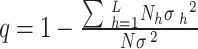
Geodetector is an effective geographic model for detecting spatial heterogeneity and explaining spatial driving factors³⁹. In this study, the factor detector was selected to quantitatively analyze the impact of various driving factors on ecological risk differentiation in the study area, and the interaction detector was used to detect the interactions between different driving factors⁴⁰. There were five modes of interaction: nonlinear weakening, one-factor nonlinear weakening, bivariate enhancement, independent, and nonlinear enhancement⁴¹. The determinant power of an explanatory variable is measured by the q value, which is calculated by:

5

Here, h = 1, …, L is the number of strata, is the number of units in a partition, N is the number of units in the whole area, is the variance of the dependent variable in the partition, and is the total variance of all dependent variables. The range of q is [0, 1]. The larger the value of q, the stronger the explanatory power of the driving factor regarding the dependent variable and the more significant the spatial differentiation.

In this study, the dependent variable was the landscape ecological risk in different years. A total of 14 natural, social, economic, and demographic factors were used as driving factors for analysis, namely, elevation, slope, NDVI, annual precipitation, annual average temperature, land use degree, GDP, output value of the primary industry, output value of the secondary industry, output value of the tertiary industry, GDP per capita, population density, anthropogenic disturbance, and grain sown area. The analysis was carried out using R software⁴². Where the degree of anthropogenic disturbance is:

6

Here, D is the degree of anthropogenic disturbance in a grid cell, n is the total number of grid cells, is the disturbance index of the i-th type of landscape, is the area of the i-th landscape type, and S is the total area of the grid. Based on previous studies^43,44, the disturbance index of various land use types was assigned. Specifically, the values for agricultural and industrial production spaces were 0.675 and 0.98, respectively. The values for woodland, grassland, water bodies, and other ecological spaces were 0.55, 0.58, 0.25, and 0.1, respectively. The value for urban and rural living spaces was 0.95.

The degree of land use is calculated as⁴⁵:

7

Here, L is the degree of land use. n is the number of landscape types in the PLEs. is the area of the i-th type of the PLEs. denotes the total area of the unit. is the land use intensity coefficient of the i-th type of the PLEs. The ecological space of unused land was assigned a value of 1, the woodland, grassland, and water had a value of 2, the agricultural space had a value of 3, and the industrial production land and urban and rural living space had a value of 4.

Results

Evolution characteristics of land use in the PLEs

Figure 2 shows the distribution of landscape types in Southwest China in 2000, 2010, and 2020. The total study area is 13.76 × 10⁵km², and the ecological space is the main component of the study area. In 2020, the area of the ecological space was 1,014,238.6 km², accounting for 74.35% of the total area. The production space had an area of 334,935.87 km², or 24.55% of the total area. The area of the living space was the smallest (14917.97 km²), accounting for only 1.1% of the total area. Specifically, woodland, agricultural land, and grassland were the primary landscape types in each space. The area of woodland remained above 48% of the total area, and the agricultural land area was about 24%. The area of grassland was slightly lower than that of agricultural land, followed by unused land, water bodies, urban living space, and rural living space. The area of the industrial production space was the smallest, accounting for less than 0.6% of the total area.

Fig. 2.

Distribution of the PLEs in Southwest China in (a)2000, (b) 2010, and (c)2020. (created by ArcMap, version 10.7, http://www.arcgis.com/).

From the area of each landscape type in 2000, 2010, and 2020 (Table 3), the grassland and other ecological spaces continued to shrink from 2000 to 2020, with a decrease of 12,686 km²and 418.02 km², respectively. The area of agricultural land decreased dramatically at first and then rebounded slightly, leading to a total decrease of 2537.34 km². The woodland area first increased and then decreased, resulting in little change in the area. The area of water bodies, industrial production space, urban living space, and rural living space increased continuously, with an increase of 3318.87, 6583.46, 3842.66, and 1128.25 km², respectively. Overall, the distribution characteristics of various functional types were characterized by a high proportion of ecological space and production space and a small proportion of living space. Specifically, urban living space and industrial production space expanded rapidly by 2.4 and 9.8, respectively, times from 2000 to 2020.

Table 3.

Variation of different land use types from 2000 to 2020.

PLEs	Area (km2)			Change (km2)			Ratio
	2000	2010	2020	2000–2010	2010–2020	2000–2020
Agricultural production space	330141.34	327115.27	327,604	−3026.08	488.73	−2537.34	0.99
Industrial production space	748.41	2267.87	7331.87	1519.46	5064	6583.46	9.80
Woodland ecological space	663741.19	673453.99	664,419	9712.8	−9034.99	677.81	1.00
Grassland ecological space	328381.26	316875.32	315,695	−11505.94	−1180.32	−12686.26	0.96
Water ecological space	11463.13	12750.02	14,782	1286.89	2031.98	3318.87	1.29
Other ecological space	19760.62	19370.19	19342.6	−390.43	−27.59	−418.02	0.98
Urban living space	2832.99	4543.81	6675.65	1710.82	2131.84	3842.66	2.36
Rural living space	7114.07	7889.97	8242.32	775.9	352.35	1128.25	1.16

Landscape ecological risk assessment

According to the distribution characteristics of the Ecological Risk Index (ERI) in each period, the ecological risks of the study area were divided into 5 intervals through the equal interval classification method: very low-risk (0.16 < ERI), low-risk (0.16 ≤ ERI < 0.19), moderate-risk (0.19 ≤ ERI < 0.22), high-risk (0.22 ≤ ERI < 0.25), and very high-risk (ERI ≥ 0.25). The average value of the ERI decreased from 0.2059 to 0.2052 over the period 2000–2010, and the index increased significantly to 0.2061 over the period 2010–2020, with a slight overall fluctuation in the average value of the ERI over the period 2010–2020 (Fig. 3). The landscape ecological risk showed significant spatial differences. Specifically, the very high-risk areas were mainly in the northeast area, which is the Sichuan Basin. The high-risk areas were in the central and northeast regions adjacent to the very high-risk areas. The low-risk areas were mainly in the west and south of the study area. The very low-risk areas were scattered in the middle of the low-risk areas.

Fig. 3.

Spatial distribution of landscape ecological risks in Southwest China in (a) 2000, (b) 2010, and (c) 2020, (d) shows the area proportion statistics of each risk level. (created by ArcMap, version 10.7, http://www.arcgis.com/).

Table 4; Fig. 4show that the moderate-risk area was the largest, accounting for more than 39% of the total area, followed by low-risk, high-risk, and very high-risk areas. The very low-risk area was the smallest. According to the landscape ecological risk transition matrix, the very low-risk, low-risk, and high-risk areas gradually shifted towards the moderate-risk area from 2000 to 2020. Specifically, the very high-risk, high-risk, and low-risk areas decreased by 1.20%, 0.61%, and 0.78%, respectively. The low-risk areas increased first and then decreased, with an overall decrease of 11900.5 km² (0.87%). The moderate-risk areas increased by 47110.80 km² (3.45%).

Table 4.

Area of regions with varying landscape ecological risk levels in Southwest China(km²).

Ecological risk interval	2000	2010	2020	2000–2020
Very low	66303.25	70540.00	54402.75	-11900.5
Low	401426.00	393812.00	390811.80	-10614.2
Moderate	535218.00	556318.30	582328.80	47110.8
High	224535.00	217938.00	216266.00	-8269
Very high	136928.30	125802.00	120600.00	-16328.3

Fig. 4.

Sankey diagram of landscape ecological risk transition matrix from 2000 to 2020.

Spatial autocorrelation

The results of the global spatial autocorrelation are shown in Fig. 5. The values for Moran’s I in the study area in 2000, 2010, and 2020 were 0.602, 0.603, and 0.547, respectively (p ≤ 0.05). The index values were all greater than 0.5, indicating that the ecological risks had a significant positive spatial correlation and aggregation characteristics, that is, the landscape ecological risks of adjacent units were similar and affected each other. The Moran’s I datapoints were mainly distributed in quadrants one and three, showing a “high-high” and “low-low” aggregation pattern. The Moran’s I showed a downward trend in the past 20 years, and some points in quadrant one were dispersed, indicating that the spatial aggregation of the regional landscape ecological risks gradually weakened with time. This was particularly true in some assessment units.

Fig. 5.

Scatter plot of the Moran’s I values in the study area in (a) 2000, (b) 2010, and (c) 2020.

The local spatial autocorrelation (Fig. 6) further verified the above results. The number of “high-high” and “low-low” autocorrelation types of the landscape ecological risk in the study area showed a downward trend from 2000 to 2020, and the number of “low-high” and “high-low” autocorrelation types showed little change. The area with insignificant spatial autocorrelation gradually increased. From the perspective of spatial distribution, the “high-high” areas were mainly in the northeastern part of the study area, with a small area distributed in the middle, while the “low-low” areas were mainly in the west and southeast. In general, there was a high consistency between the aggregation pattern and the spatial distribution of the landscape ecological risk areas.

Fig. 6.

LASA aggregation map of the landscape ecological risks in the study area in (a) 2000, (b) 2010, and (c) 2020. (created by Geoda, version 1.16, https://geodacenter.github.io/).

Landscape ecological network construction

Resistance surfaces were established using the MCR model (Fig. 7a), revealing the highest ecological resistance in the northeastern region and low resistance in the southwestern region. The ecological network pattern of the study area is illustrated in Fig. 7b. According to the MSPA model, 13 large-scale core ecological sources, each larger than 10 km², were identified, primarily distributed in the Guizhou, Yunnan, and Guangxi regions. Potential ecological corridors were identified by simulating the minimum depletion paths between the ecological sources. Radial ecological corridors were identified through hydrological analyses. After merging or deleting some of the overlapping corridors, 63 potential ecological corridors and 42 radial ecological corridors were identified. The average lengths of the potential and radial ecological corridors were 147 km and 110 km, respectively. A total of 156 ecological nodes were identified at the intersections of ecological corridors with each other, tertiary or higher rivers, and national highways. The ecological nodes in the southwestern part of the study area are relatively dense. These nodes are essential for species migration and material-energy exchange in the ecosystem and should be protected and utilized. The northwestern and northeastern parts of the study area have the highest ecological resistance, severely obstructing energy flow within the ecosystem and reducing connections with the ecological corridors of ecological sources, making them relatively isolated. To improve the ecological service value of high-resistance areas, measures such as ecological node protection and corridor restoration should be implemented to enhance landscape connectivity across the region.

Fig. 7.

Spatial distribution of minimum cumulative resistance surface (a) and ecological networks (b) in the study area. (created by ArcMap, version 10.7, http://www.arcgis.com/).

Quantitative driving factor analysis of the spatiotemporal differentiation of the landscape ecological risks

The correlation coefficients between the ecological risk index and the influencing factors varied greatly across the study area (Fig. 8). In the three periods of data, the degree of land use, GDP, the output value of the primary, secondary, and tertiary industries, population density, degree of anthropogenic interference, and sown area of grain were significantly and positively correlated with the ecological risk index (P < 0.01). Conversely, elevation, slope, NDVI, annual average rainfall, and annual average temperature were significantly and negatively correlated with the ecological risk index, with elevation, slope, and annual average temperature showing significant negative correlations only in 2020. In 2000 and 2010, NDVI was positively correlated with the ecological risk index. In 2020, significant negative correlations were observed with elevation, slope, and mean annual temperature. Among the three periods, the highest correlations with the ecological risk index were found with the the degree of land use, degree of anthropogenic disturbance, and the value of primary industrial output. These correlations decreased over time, with coefficients of 0.555, 0.382, and 0.281 in 2020, respectively.

Fig. 8.

Correlation analysis of ecological risk indices with driver indicators. E: elevation, S: slope, N: NDVI, AP: annual precipitation, AT: average annual temperature, LU: degree of land use, G: GDP, PI: output value of the primary industry, SI: output value of the secondary industry, TI: output value of the tertiary industry, GP: GDP per capita, P: population density, AD: degree of anthropogenic disturbance, GS: grain sown area.

Taking all the driving factors as independent variables, RF and Geodetector models of the landscape ecological risk index in the study area were constructed to analyze the effects of these factors on the landscape ecological risk pattern in Southwest China in 2000, 2010, and 2020. The importance assessment of the driving factors calculated by the RF and the q-value ranking results calculated by the Geodetector were normalized and compared (Fig. 9). The RF importance and Geodetector q-value results show similar patterns. In 2000, the Geodetector calculated that the five factors with the strongest explanatory power were anthropogenic disturbance, land use degree, population density, sown area of grain, and GDP, while the RF model identified anthropogenic disturbances, land use degree, annual precipitation, average annual temperature, and GDP per capita as the most important variables. In 2010 and 2020, anthropogenic disturbance and land use degree remained the main drivers, while elevation, slope, and NDVI had the lowest explanatory power for the risk index. Notably, both approaches demonstrate an increasing impact of the area allotted for grain production on ecological risk over time. This trend may be attributed to the policy of returning farmland to forest. In summary, anthropogenic factors and production activities are the main drivers of the evolution of landscape ecological risk in Southwest China, demonstrating the significant influence of production and living spaces on regional landscape ecological risk.

Fig. 9.

The radial histogram of the driving factors obtained by RF and Geodetector in (a) 2000, (b) 2010 and (c) 2020. E: elevation, S: slope, N: NDVI, AP: annual precipitation, AT: average annual temperature, LU: degree of land use, G: GDP, PI: output value of the primary industry, SI: output value of the secondary industry, TI: output value of the tertiary industry, GP: GDP per capita, P: population density, AD: degree of anthropogenic disturbance, GS: grain sown area.

There are differences in the importance and q-value ordering of the influencing factors at different spatiotemporal scales, and the spatiotemporal variability of landscape ecological risk may be influenced by the superposition of diverse factors. Therefore, this paper adopts an interaction detector to further analyze these effects based on single-factor detection using the Geodetector model. The analysis using the interaction detector showed that the interaction mechanisms of factors driving spatiotemporal changes in ecological risk varied significantly (Fig. 10). The interaction types were mainly nonlinear enhancement and two-factor enhancement, indicating a significant effect of multi-factor superposition on the spatial differentiation of landscape ecological risk in the study area. In 2000, the interaction between anthropogenic disturbance and annual precipitation had the greatest effect on the spatial differentiation of ecological risk, with a q-value of 0.829. This was followed by the interactions between anthropogenic disturbance and GDP, and between anthropogenic disturbance and annual average temperature. In 2010, the interaction between anthropogenic disturbance and annual average temperature had the greatest effect on the spatial differentiation of ecological risks, with a q-value of 0.805. This was followed by the interactions between anthropogenic disturbance and the output value of the tertiary industry, and between anthropogenic disturbance and GDP, both with q-values of 0.8. In 2020, the interaction between anthropogenic disturbance and annual average temperature had the greatest effect on the spatial differentiation of ecological risks, with a q-value of 0.76. The interactions between anthropogenic disturbance and the output value of the tertiary industry, and between anthropogenic disturbance and GDP, both had q-values of 0.757. In general, the evolution of landscape ecological risk is not dominated by a single pair of factors. Instead, the interactions of anthropogenic disturbances with regional climate and economic activity have the greatest impact on landscape ecological risk. The explanatory power of the interaction of each pair of factors tended to decrease over time.

Fig. 10.

Detection results of the interaction of driving factors obtained by Geodetector in (a) 2000, (b) 2010, and (c) 2020. E: elevation, S: slope, N: NDVI, AP: annual precipitation, AT: average annual temperature, LU: degree of land use, G: GDP, PI: output value of the primary industry, SI: output value of the secondary industry, TI: output value of the tertiary industry, GP: GDP per capita, P: population density, AD: degree of anthropogenic disturbance, GS: grain sown area.

Discussion

Spatial and temporal assessment of ecological risk in the landscape

In this study, multiple landscape indices were used to comprehensively assess ecological risk and establish the relationship between the distribution of PLEs and ecological risk, providing an effective method for assessing the spatial and temporal patterns of ecological risk. The landscape ecological risk in Southwest China showed significant positive spatial correlation and aggregation characteristics. In general, the risk was higher in the northeast and lower in the southwest. The differentiation of landscape ecological risks was closely related to the distribution of PLEs⁴⁶. High-risk areas were mainly in Sichuan, Guizhou, and Chongqing. Specifically, concentrated and contiguous high-risk areas were located in the northeastern part of the study area, particularly the Sichuan Basin. Due to its unique topographical features, the Sichuan Basin has flat terrain and a suitable environment for farming, which results in high ecological vulnerability due to concentrated agricultural production space. Strong anthropogenic disturbance combined with natural disasters lead to the highest ecological risk^47,48. Moreover, due to the large amount of sandy and bare land in western and northern Sichuan Province, vegetation coverage and biodiversity are low⁴⁹, making the ecological environment fragile and increasing ecological risk. Since there are more water resources in the western part, the ecological risk is lower than in the northern part. In the western part of Guizhou Province, forests, grasslands, and water resources are present, yet the primary land use remains agricultural production, resulting in slightly higher ecological risk. As the capital city of Guizhou, Guiyang experienced rapid urbanization and industrialization, which resulted in increased landscape fragmentation and decreased ecosystem service functions, causing a shift towards high-risk levels^16,50. Notably, in a few high-risk areas, such as southwest Chongqing, the risk tends to shift towards a medium-risk level despite the expansion of urban living spaces, possibly due to intra-city greening and better connectivity in the urban landscape¹⁷. The very low-risk and low-risk areas are mainly in Yunnan, Guangxi, and Sichuan Provinces, where basins are widely distributed.Suitable subtropical climatic conditions and sufficient rainfall have led to a structurally stable vegetation landscape^46,51.Additionally, local governments have placed great importance on ecological protection⁵², resulting in low ecological risk. In western Guangxi Province, the transition of woodland and grassland to agricultural production space has increased landscape vulnerability and fragmentation, resulting in a rising trend in ecological risks. Spatial autocorrelation showed a trend of very high-risk and very low-risk areas changing from aggregation to dispersion patterns, with moderate-risk areas gradually expanding into low-risk and high-risk areas.

Recommendations for the construction of landscape ecological networks

The MSPA model was used to identify large core ecological sources in the study area, mainly distributed in the Yunnan and Guangxi regions. As the primary habitat for species in the ecosystem, ecological source should strengthen the connection between core landscape patches and surrounding small patches, expand patch areas, and reduce landscape fragmentation⁵³. The ecological network constructed using the MCR model showed that the ecological corridors in the southwestern part of the study area were denser and had good landscape connectivity, which facilitated energy flow and species migration between patches⁵⁴. Moreover, the northeastern portion of the study area is less connected to large ecological sources in the southwestern portion due to high ecological resistance and poor landscape connectivity. Ecological nodes are important functional components in the construction of ecological networks, playing an essential role in species migration and dispersal, and should be given enhanced protection and construction in network structures⁵⁵. Therefore, in constructing landscape ecological networks, the quality of arable land should be improved, town boundaries controlled, land use conflicts coordinated, and emphasis placed on reducing ecological risks in high-risk areas. Potential ecological corridors and radiating ecological corridors important for biodiversity conservation should be strictly controlled and protected. Additionally, attention should be paid to maintaining ecologically fragile areas such as rivers and roads. Based on the protection of core patches and ecological corridors, the protection of ecological nodes should be improved to enhance connectivity between patches in the low-risk southwestern and high-risk southeastern zones. Eventually, the connectivity and stability of landscape elements in medium-risk, high-risk, and very high-risk areas across the entire study area will be improved, optimizing the overall structure of the ecological network.

Analysis of the drivers of landscape ecological risk and policy recommendations

Consistent with previous studies, anthropogenic disturbance was the main driving factor for landscape pattern and spatial function transformation in Southwest China, as well as changes in ecological risk indices^31,56. In addition, the degree of land use directly reflects the landscape structure and ecosystem vulnerability, significantly impacting ecological risks⁵⁷. Natural factors are the basis for regional landscape differentiation. Factor detection revealed that topographic and climatic factors alone did not have strong explanatory power for ecological risks. However, when interaction with anthropogenic disturbance, the explanatory power was greatly enhanced, with climatic factors showing the most significant increase. Although NDVI is closely related to vegetation coverage changes, it has the weakest explanatory power for ecological risk in the study area. This may be because the study area is dominated by ecological space, and small changes in the spatial structure of the vegetation landscape have little effect on ecological risk⁵⁸. Overall, production space was the main driving force for the spatiotemporal differentiation of landscape ecological risks in Southwest China, with anthropogenic disturbance being a key driving factor. It is worth noting that Geodetector results showed a decline in the explanatory power of all driving factors for ecological risk, except for a few factors such as NDVI. This may further explain the shift of landscape ecological risk from aggregation to dispersion patterns. Due to the increase in disturbance sources such as natural disasters, nature reserves, and road risks, the explanatory power of the main driving factors was weakened⁵⁸, which is a significant issue in the ecological development of Southwest China.

To summarize, the focus should be on solving the contradiction between human activities and land use during regional development and minimizing the negative impacts of anthropogenic disturbance on ecological protection⁵⁹. For very high-risk and high-risk areas, policies and regulations should encourage the return of farmland to forest and grassland, expand vegetation coverage, improve the quality of cultivated land, strengthen water protection, control urban development boundaries, protect land resources, and reduce landscape fragmentation. For moderate-risk areas, it is essential to optimize the spatial layout of PLEs, improve land use efficiency to coordinate social-economic development with ecological protection, and prevent the transition of ecological risks. For very low-risk and low-risk areas, the protection of woodland, grassland, and water ecological spaces should be strengthened, and ecological environmental protection and monitoring should be carried out to maintain landscape stability and avoid an increase in ecological risks. For the entire study area, the protection of ecological sources, corridors, and nodes in the ecological network should be strengthened to enhance landscape connectivity and the stability.

Limitations and future perspectives

This study presents a methodology for assessing changes in ecological risk in regional landscapes, optimising the spatial pattern of ecological networks, and quantifying how ecological, living and production drivers influence the spatial evolution of ecological risk patterns from the perspective of PLEs. Compared to previous studies, this study introduces several methodological innovations. Firstly, previous landscape ecology studies tend to conduct risk assessments based on current land use status, while this study adopts the function-oriented land use classification method of PLEs to assess the ecological risk of the study area. Secondly, when constructing the ecological safety network, this study utilizes the risk assessment results derived from various landscape pattern indicators as the ecological resistance surface, making it more scientifically sound and reasonable. Finally, previous landscape-driven studies mainly focused on single factors such as land use or climate change, without fully considering human activities and the interactions among factors. The study results can provide a reference for the relationship between regionally balanced urbanization and ecological security. However, this study has limitations and potential areas for future improvement. Firstly, there are overlaps and deviations in the spatial categorization of PLEs. For example, grassland is ecological land, but pastureland has a production function, and woodland is classified as ecological space but also has a production function. Urban green spaces are also ecological spaces, but since they are located in urban areas, they are classified as urban living spaces. Similarly, production space is included in living space. The boundaries of production, living, and ecological spaces cannot be clearly delineated. Therefore, applying this research method to different regions should fully consider the dominant functions of regional land. Secondly, the landscape risk assessment conducted in this study is primarily based on landscape pattern indicators. These indicators typically consider only the intrinsic function of the patch and are related to the size of the patch unit⁶⁰. Therefore, the results of this study may be different in other regions, and future studies should consider the introduction of dynamic landscape indicators in the risk assessment framework based on spatiotemporal scales. Finally, the selection of drivers in this study is limited and their interactions are complex. Therefore, it is necessary to consider additional drivers, such as biomass and carbon storage, and incorporate them into the driver index system in future studies. In conclusion, this study provides a valuable case for ecological risk assessment and driver analysis under land use transition, offering a more targeted decision-making strategy for ecological risk management.

Conclusions

In this study, we assessed the spatiotemporal evolution of ecological risk in Southwest China from 2000 to 2020 using PLEs land use data. On this basis, the landscape ecological network in 2020 was optimised using MSPA and MCR models. Finally, the driving mechanisms behind ecological risks were explored using RF and Geodetector models. The study draws the following conclusions: (1) Ecological space is the main functional type of the landscape in Southwest China. From 2000 to 2020, the expansion of industrial production space and urban living space has been the main evolutionary feature of PLEs. (2) The landscape ecological risk index has not changed much in the last 20 years, but there are significant changes in different zoning levels. It shows that the areas of high-risk and low-risk zones have shrunk, while the area of medium-risk zones has gradually expanded. The distribution of ecological risk has obvious regional characteristics, with higher risk levels in the northeast and lower risk levels in the southwest. In addition, ecological risk has a significant positive spatial correlation, the spatial aggregation of ecological risk decreases over time, and the connection between landscape units gradually weakens. (3) A total of 105 potential ecological corridors and radial ecological corridors were identified, and 156 ecological nodes at corridor intersections and corridors with rivers and national highways were identified. To enhance landscape connectivity, ecological corridors and nodes should be protected and utilized with emphasis. (4) Anthropogenic disturbance and land use degree have the highest explanatory power for ecological risk changes in Southwest China, and the interaction of anthropogenic disturbance with climate and economy is the main factor influencing the spatiotemporal differentiation of landscape ecological risk. In conclusion, the results of this study emphasize the importance of coordinated development of land use and ecological protection and common planning in regional land management. Decision-makers should strive to reduce the impacts of various risk factors on ecosystem security during land space optimization.

Author contributions

H.C. (Hui Chen) conducted the cartography and wrote the original draft of the manuscript. Meanwhile, T.H. and Z.G. formulated the methodology and edited the manuscript. Additionally, H.C. (Hongxing Chen), X.H., and S.Z. gathered and pre-processed the data presented in this paper. All authors have read and agreed to the published version of the manuscript.

Data availability

The data that support the findings of this study are openly available in Zenodo at https://doi.org/10.5281/zenodo.13643266, reference number https://zenodo.org/records/13643266.

Declarations

Competing interests

The authors declare no competing interests.

References

- 1.Liu, Y., Fang, F. & Li, Y. Key issues of land use in China and implications for policy making. Land. Use Policy. 40, 6–12 (2014). [Google Scholar]
- 2.Fu, J., Gao, Q., Jiang, D., Li, X. & Lin, G. Spatial–temporal distribution of global production–living–ecological space during the period 2000–2020. Sci. Data. 10, 589 (2023). [DOI] [PMC free article] [PubMed] [Google Scholar]
- 3.Zhang, Z. & Li, J. Spatial suitability and multi-scenarios for land use: Simulation and policy insights from the production-living-ecological perspective. Land. Use Policy. 119, 106219 (2022). [Google Scholar]
- 4.Li, Y. et al. The role of land use change in affecting ecosystem services and the ecological security pattern of the Hexi regions, Northwest China. Sci. Total Environ.855, 158940 (2023). [DOI] [PubMed] [Google Scholar]
- 5.Zhang, Y., Li, Y., Lv, J., Wang, J. & Wu, Y. Scenario simulation of ecological risk based on land use/cover change – a case study of the Jinghe county, China. Ecol. Ind.131, 108176 (2021). [Google Scholar]
- 6.Ayre, K. K. & Landis, W. G. A bayesian Approach to Landscape Ecological Risk Assessment Applied to the Upper Grande Ronde Watershed, Oregon. Hum. Ecol. Risk Assessment: Int. J.18, 946–970 (2012). [Google Scholar]
- 7.Liang, Y. & Song, W. Integrating potential ecosystem services losses into ecological risk assessment of land use changes: a case study on the Qinghai-Tibet Plateau. J. Environ. Manage.318, 115607 (2022). [DOI] [PubMed] [Google Scholar]
- 8.Leuven, R. S. E. W. & Poudevigne, I. Riverine landscape dynamics and ecological risk assessment. Freshw. Biol.47, 845–865 (2002). [Google Scholar]
- 9.Depietri, Y. The social–ecological dimension of vulnerability and risk to natural hazards. Sustain. Sci.15, 587–604 (2020). [Google Scholar]
- 10.Hope, B. K. An examination of ecological risk assessment and management practices. Environ. Int.32, 983–995 (2006). [DOI] [PubMed] [Google Scholar]
- 11.Wang, H. et al. Spatial-temporal pattern analysis of landscape ecological risk assessment based on land use/land cover change in Baishuijiang National nature reserve in Gansu Province, China. Ecol. Ind.124, 107454 (2021). [Google Scholar]
- 12.Karimian, H., Zou, W., Chen, Y., Xia, J. & Wang, Z. Landscape ecological risk assessment and driving factor analysis in Dongjiang river watershed. Chemosphere. 307, 135835 (2022). [DOI] [PubMed] [Google Scholar]
- 13.Shi, Y., Feng, C. C., Yu, Q., Han, R. & Guo, L. Contradiction or coordination? The spatiotemporal relationship between landscape ecological risks and urbanization from coupling perspectives in China. J. Clean. Prod.363, 132557 (2022). [Google Scholar]
- 14.Liu, D., Chen, H., Zhang, H., Geng, T. & Shi, Q. Spatiotemporal Evolution of Landscape Ecological Risk Based on Geomorphological Regionalization during 1980–2017: A Case Study of Shaanxi Province, China. Sustainability 12, 941 (2020).
- 15.Mansori, M., Badehian, Z., Ghobadi, M. & Maleknia, R. Assessing the environmental destruction in forest ecosystems using landscape metrics and spatial analysis. Sci. Rep.13, 15165 (2023). [DOI] [PMC free article] [PubMed] [Google Scholar]
- 16.Dadashpoor, H., Azizi, P. & Moghadasi, M. Land use change, urbanization, and change in landscape pattern in a metropolitan area. Sci. Total Environ.655, 707–719 (2019). [DOI] [PubMed] [Google Scholar]
- 17.Velázquez, J. et al. Planning and selection of green roofs in large urban areas. Application to Madrid metropolitan area. Urban Forestry Urban Green.40, 323–334 (2019). [Google Scholar]
- 18.Jongman, R. H. G., Külvik, M. & Kristiansen, I. European ecological networks and greenways. Landsc. Urban Plann.68, 305–319 (2004). [Google Scholar]
- 19.Blasi, C. et al. The concept of land ecological network and its design using a land unit approach. Plant. Biosystems. 142, 540–549 (2008). [Google Scholar]
- 20.Zhao, S., Ma, Y., Wang, J. & You, X. Landscape pattern analysis and ecological network planning of Tianjin City. Urban Forestry Urban Green.46, 126479 (2019). [Google Scholar]
- 21.Chen, J. et al. Study on landscape ecological risk assessment of hooded Crane breeding and overwintering habitat. Environ. Res.187, 109649 (2020). [DOI] [PubMed] [Google Scholar]
- 22.Zhu, K. et al. Identification and prevention of agricultural non-point source pollution risk based on the minimum cumulative resistance model. Global Ecol. Conserv.23, e01149 (2020). [Google Scholar]
- 23.Pineda Jaimes, N. B., Sendra, B. & Gómez Delgado, J. Franco Plata, R. Exploring the driving forces behind deforestation in the state of Mexico (Mexico) using geographically weighted regression. Appl. Geogr.30, 576–591 (2010). [Google Scholar]
- 24.Maćkiewicz, A. & Ratajczak, W. Principal components analysis (PCA). Comput. Geosci.19, 303–342 (1993). [Google Scholar]
- 25.Luo, W. et al. Spatial association between dissection density and environmental factors over the entire conterminous United States. Geophys. Res. Lett.43, 692–700 (2016). [Google Scholar]
- 26.Hu, D., Meng, Q., Zhang, L. & Zhang, Y. Spatial quantitative analysis of the potential driving factors of land surface temperature in different centers of polycentric cities: a case study in Tianjin, China. Sci. Total Environ.706, 135244 (2020). [DOI] [PubMed] [Google Scholar]
- 27.Ngabire, M., Wang, T., Liao, J. & Sahbeni, G. Quantitative analysis of desertification-driving mechanisms in the Shiyang River Basin: Examining Interactive effects of Key factors through the Geographic detector model. Remote Sens.15, 2960 (2023). [Google Scholar]
- 28.Belgiu, M. & Drăguţ, L. Random forest in remote sensing: a review of applications and future directions. ISPRS J. Photogrammetry Remote Sens.114, 24–31 (2016). [Google Scholar]
- 29.Wang, Z., Liu, Y., Li, Y. & Su, Y. Response of Ecosystem Health to Land Use Changes and Landscape patterns in the Karst mountainous regions of Southwest China. Int. J. Environ. Res. Public Health. 19, 3273 (2022). [DOI] [PMC free article] [PubMed] [Google Scholar]
- 30.Cui, L. et al. Landscape ecological risk assessment in Qinling Mountain. Geol. J.53, 342–351 (2018). [Google Scholar]
- 31.Wang, B., Ding, M., Li, S., Liu, L. & Ai, J. Assessment of landscape ecological risk for a cross-border basin: a case study of the Koshi River Basin, central Himalayas. Ecol. Ind.117, 106621 (2020). [Google Scholar]
- 32.Rangel-Buitrago, N. & Neal, W. J. Jonge, V. N. Risk assessment as tool for coastal erosion management. Ocean. Coastal. Manage.186, 105099 (2020). de. [Google Scholar]
- 33.Hou, M. et al. Ecological Risk Assessment and Impact factor analysis of Alpine Wetland Ecosystem based on LUCC and boosted regression tree on the Zoige Plateau, China. Remote Sens.12, 368 (2020). [Google Scholar]
- 34.Cabral-Alemán, C., López-Santos, A. & Zúñiga-Vásquez, J. M. Mapping risk zones of potential erosion in the upper Nazas River basin, Mexico through spatial autocorrelation techniques. Environ. Earth Sci.80, 653 (2021). [Google Scholar]
- 35.Ghulam, A. et al. Remote sensing based spatial statistics to Document Tropical Rainforest Transition pathways. Remote Sens.7, 6257–6279 (2015). [Google Scholar]
- 36.Moran, P. a. P. The interpretation of statistical maps. J. Roy. Stat. Soc.: Ser. B (Methodol.). 10, 243–251 (1948). [Google Scholar]
- 37.Wickham, J. D., Riitters, K. H., Wade, T. G. & Vogt, P. A national assessment of green infrastructure and change for the conterminous United States using morphological image processing. Landsc. Urban Plann.94, 186–195 (2010). [Google Scholar]
- 38.Breiman, L. Random forests. Mach. Learn.45, 5–32 (2001). [Google Scholar]
- 39.Wang, J. et al. Geographical detectors-based Health Risk Assessment and its application in the neural tube defects study of the Heshun Region, China. Int. J. Geogr. Inf. Sci.24, 107–127 (2010). [Google Scholar]
- 40.Song, Y., Wang, J., Ge, Y. & Xu, C. An optimal parameters-based geographical detector model enhances geographic characteristics of explanatory variables for spatial heterogeneity analysis: cases with different types of spatial data. null. 57, 593–610 (2020). [Google Scholar]
- 41.Feng, R., Wang, F., Wang, K., Wang, H. & Li, L. Urban ecological land and natural-anthropogenic environment interactively drive surface urban heat island: an urban agglomeration-level study in China. Environ. Int.157, 106857 (2021). [DOI] [PubMed] [Google Scholar]
- 42.Cao, F., Ge, Y. & Wang, J. F. Optimal discretization for geographical detectors-based risk assessment. GIScience Remote Sens.50, 78–92 (2013). [Google Scholar]
- 43.Hill, M. O., Roy, D. B. & Thompson, K. Hemeroby, urbanity and ruderality: bioindicators of disturbance and human impact. J. Appl. Ecol.39, 708–720 (2002). [Google Scholar]
- 44.Wu, T. et al. Landscape Pattern Evolution and its response to human disturbance in a newly Metropolitan Area: a Case Study in Jin-Yi Metropolitan Area. Land. 10, 767 (2021). [Google Scholar]
- 45.Liang, T. et al. Land-Use Transformation and Landscape Ecological Risk Assessment in the Three Gorges Reservoir Region based on the production–living–ecological space perspective. Land. 11, 1234 (2022). [Google Scholar]
- 46.Huang, T., Wang, N., Luo, X. & Xu, J. Landscape ecological risks assessment of the China-Vietnam border area: the perspective of production-living-ecological spaces. Reg. Environ. Change. 24, 103 (2024). [Google Scholar]
- 47.Mo, W., Wang, Y., Zhang, Y. & Zhuang, D. Impacts of road network expansion on landscape ecological risk in a megacity, China: a case study of Beijing. Sci. Total Environ.574, 1000–1011 (2017). [DOI] [PubMed] [Google Scholar]
- 48.Kondolf, G. M. & Podolak, K. Space and Time scales in Human-Landscape systems. Environ. Manage.53, 76–87 (2014). [DOI] [PubMed] [Google Scholar]
- 49.Akomolafe, G. F. & Rosazlina, R. Land use and land cover changes influence the land surface temperature and vegetation in Penang Island, Peninsular Malaysia. Sci. Rep.12, 21250 (2022). [DOI] [PMC free article] [PubMed] [Google Scholar]
- 50.Liao, J. et al. Assessment of urbanization-induced ecological risks in an area with significant ecosystem services based on land use/cover change scenarios. Int. J. Sustainable Dev. World Ecol.25, 448–457 (2018). [Google Scholar]
- 51.Ran, P. et al. Exploring changes in landscape ecological risk in the Yangtze River Economic Belt from a spatiotemporal perspective. Ecol. Ind.137, 108744 (2022). [Google Scholar]
- 52.Zheng, K. et al. Temporal and spatial variation of landscape ecological risk and influential factors in Yunnan border mountainous area. Acta Ecol. Sin.42, 7458–7469 (2022). [Google Scholar]
- 53.Mitchell, M. G. E. et al. Reframing landscape fragmentation’s effects on ecosystem services. Trends Ecol. Evol.30, 190–198 (2015). [DOI] [PubMed] [Google Scholar]
- 54.Velázquez, J. et al. Planning Restoration of Connectivity and Design of Corridors for Biodiversity Conservation. Forests. 13, 2132 (2022). [Google Scholar]
- 55.Guan, D., Jiang, Y. & Cheng, L. How can the landscape ecological security pattern be quantitatively optimized and effectively evaluated? An integrated analysis with the granularity inverse method and landscape indicators. Environ. Sci. Pollut Res.29, 41590–41616 (2022). [DOI] [PubMed] [Google Scholar]
- 56.Yang, Y. & Song, G. Human disturbance changes based on spatiotemporal heterogeneity of regional ecological vulnerability: a case study of Qiqihaer city, northwestern Songnen Plain, China. J. Clean. Prod.291, 125262 (2021). [Google Scholar]
- 57.Wang, A. et al. Spatial-temporal dynamic evaluation of the ecosystem service value from the perspective of production-living-ecological spaces: a case study in Dongliao River Basin, China. J. Clean. Prod.333, 130218 (2022). [Google Scholar]
- 58.Wang, S., Tan, X. & Fan, F. Landscape Ecological Risk Assessment and Impact factor analysis of the Qinghai–Tibetan Plateau. Remote Sens.14, 4726 (2022). [Google Scholar]
- 59.Tian, F., Li, M., Han, X., Liu, H. & Mo, B. A production–living–ecological space model for land-use optimisation: a case study of the core Tumen River region in China. Ecol. Model.437, 109310 (2020). [Google Scholar]
- 60.Zhang, L., Peng, J., Liu, Y. & Wu, J. Coupling ecosystem services supply and human ecological demand to identify landscape ecological security pattern: a case study in Beijing–Tianjin–Hebei Region, China. Urban Ecosyst.20, 701–714 (2017). [Google Scholar]
Associated Data
This section collects any data citations, data availability statements, or supplementary materials included in this article.
Data Availability Statement