Mining, refining, and QSAR analysing the nanoinformatics in EPA NaKnowBase

Abstract

Concerns about the safety of manufacturing and using engineered nanomaterials (ENMs) have been increasing as the technology continues to expand. Efforts have been underway to investigate the potentially harmful effects of ENMs without carrying out the challenging empirical studies. To make such investigations possible, the US EPA Office of Research and Development (ORD) developed the nanomaterial database NaKnowBase (NKB) containing the detail of hundreds of assays conducted and published by ORD scientists experimentally investigating the environmental health and safety effects of ENMs (nanoEHS). This article describes specifics of the effort to mine, refine, and analyse the NKB. Here we use a quantitative structure activity relationship (QSAR) analysis, using a random forest of decision trees to predict the in vitro cell viability effects that occur upon exposure to ENMs that are similar in composition and structure and implement a set of laboratory conditions. These predictions are confirmed using the Jaqpot cloud platform developed by the National Technical University of Athens, Greece (NTUA) where nanoEHS effects are investigated with scientists working together globally.

Graphical Abstract

The EPA nanoQSAR model predicts the impacts of in vitro cell viability following exposure to certain nanomaterials.

Overview

Over the past forty years, nanotechnology has developed radically, so that now science is designing complex nanostructures and materials with unique properties at the molecular level. In general, engineered nanomaterials (ENMs) are defined to be 100 nanometers (nm) and less. These include integrated circuits (IC)¹ designed for computer chips, now on the order of 5 nm, high tensile strength single- and multi-walled carbon nanotubes (SWCNT, MWCNT) ^2,3 with diameters from 0.5 to 50 nm, quantum dots⁴ from 1.0 to 10.0 nm in size and twisted ‘magic-angle’ graphene-like superconducting layered planes.⁵ These examples reveal a manifold of new areas of research and development.

With these radical advances in nanotechnology, the European Union (EU) and the United States (US) recently published a nanoinformatics roadmap⁶ to guide nanoinformatics development, nanomaterial risk assessment and governance issues over the next ten years. Substantial concerns have been raised about the possible adverse health effects and safety of ENMs when released to the environment (nanoEHS)⁷ and research projects have been initiated to develop innovative and integrated tools for nanosafety assessment.⁸

The United States Environmental Protection Agency (US EPA) Office of Research and Development (ORD) launched a research program to understand the potential environmental impacts of ENM wastes released all through the manufacturing and commercial uses of ENMs. Under this program, research was performed by ORD scientists to establish the effects of different ENMs released to the environment. Results of this research have been published in various scientific journals over the past ten years.^9–14

The relational database NaKnowBase (NKB) was developed by ORD to take the results of this research and connect the physical and chemical characteristics of the ENMs studied with any adverse effects encountered.¹⁵ An article was recently published announcing the official release of NKB.¹⁶ Boyes, et al. (2022)¹⁶ presents extensive details about the background, design, structure, and building of the ORD database. Using regression algorithms like those implemented in quantitative structural–activity relationship (QSAR) analysis, it is possible to make predictions to estimate the adverse effects using the ENMs found in NKB.

There are many ways to process the data within NKB to make predictions. SQLAlchemy (https://www.sqlalchemy.org/)¹⁷ is a Python structured query language (SQL) toolkit that makes the power and flexibility of SQL available to Python developers. It provides a way to access SQL databases directly from Python using SQL queries to generate the data used for regression models. Using SQLAlchemy, it was found effective, and preferrable to accessing the database at runtime, to download and save all of the data into a comma-separated values (CSV) file for runtime access. =. This downloaded file needs to be updated periodically to ensure changes to the database are implemented.

To make predictions, regression algorithms from Python’s ScikIt-learn Machine Learning Library¹⁸ (https://scikit-learn.org/stable/) (sklearn) expect machine learning modeling to be performed with data in a two-dimensional numerical array with one sample in each row. However, when a mySQL relational database is simply flattened into a CSV file, many consecutive rows of the file may belong to the same sample. At some point, a procedure of adding columns known as pivoting must be performed on this data to place consecutive rows of the same sample into a single row. This gives one row for each sample and makes it easier to transfer the rows into a two-dimensional array of samples prior to regression analysis. For our analysis, it was chosen to first pivot in mySQL script and then download to a CSV file where each row of the file represents one unique assay sample.

Once the CSV file has been generated, it was necessary to pre-process data before any predictions can be made using QSAR analysis. For example, NKB was designed to accept many conventions of the eNanoMapper^19,20 ontologies; one of which allows values to be entered along with their associated units. Before QSAR analysis can be done, the values and units of a property must be converted to the same units so they may be compared. In a similar way, categorical data (e.g., “spherical”, “amorphous”, “crystalline”) must be encoded into numerical data to contribute to the analysis.

After the steps listed above have been completed, all columns of the spreadsheet are numerical. One column is the target of prediction, and the other columns are descriptors used for QSAR analysis. Each row of this spreadsheet is a sample used to train or test models that are built. The QSAR analysis is accomplished using sklearn’s RandomForestRegressor routine.

So far, we have discussed datamining and refining NKB data for our analyses, and prediction of the adverse effect of new ENMs like those in NKB using QSAR analyses. The predictions that are made here are compared with observed values to evaluate the accuracy of the model selected. In a similar way, cross-validation is performed over models built from different datasets to estimate the variation of the accuracy measured. The mySQL script and Python files used to execute these processes are provided in EPA’s nanoQSAR²¹ repository (https://www.github.com/usepa/nanoQSAR).

The last part of this article shows how these predictions can be achieved by non-technical users in. Additionally, EPA’s nanoQSAR has been provided to the National Technical University of Athens (NTUA), Greece to predict the in vitro cell viability following exposure to nanomaterials, using the Jaqpot cloud platform (https://app.jaqpot.org/),²² an online interface for models that predict nanoEHS effects.

Datamining NKB

Most algorithms for regression analysis assume the training and testing of samples are input in a simple spreadsheet format, where one sample is expected in each row. However, the relational database structure of NKB is a more complicated structure, and must first be parsed to allow for specific formatting. To enable regression analysis of the data within NKB, multiple SQL script files transform the NKB into a simple spreadsheet format held within a CSV file.

Relational databases are made from many different tables that have primary and foreign keys pointing to records in each linked table. There are many different connections between records in the tables that are determined by these keys. The graphical representation shown in Fig. 1, adopted from Boyes, et al. (2022),¹⁶ illustrates the 11 tables that constitute NKB, where each element of the figure represents one of the tables. More details about each element are shown in Table 1.

Fig. 1.

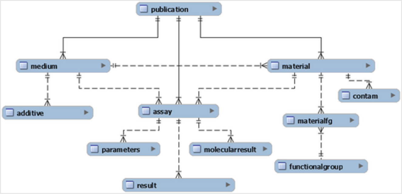
Overview of the NKB MySQL structure: the lines indicate the nature of each relationship. Each relationship is of a one-to-many nature, where the end with two lines is “ one” and the end with a triangle is “ many ”, such as one publication being able to have many mediums (adopted from Boyes, et al. (2022)). ¹⁶

Table 1.

Outline table: an overview of the data tables in NKB, with a brief description of the general type or category of data collated in each table

Data tables in NaKnowBase	Description
Publication	Identification and metadata of the published manuscript from which the data originated
Medium	The medium in which the nanomaterial was tested (e.g., water, saline, cell culture medium, etc.)
Additive	Any substances that may have been added to the media (e.g., FBS, strep/pen)
Material	The composition of the nanomaterial and any physiochemical parameters reported
Contam	Any contaminants of the test material reported
Materialfg	Functional groups affixed to primary test material and the method of affixation
Functionalgroup	Identities of functional groups in database (e.g., alcohol groups)
Assay	The type of test system used (e.g., in vitro test system, electron microscopy)
Parameters	Parameters manipulated in the experiment (e.g., dose/concentration tested, test time, etc.)
Result	Measured results linked to the assays and parameters employed
Molecularresult	Pointer to results from complex assays such as genomics, proteomics, etc., that are deposited elsewhere

Fig. 1 and Tables 1–5 in this article were shown originally in the article announcing the official release of NKB.¹⁶

Table 5.

Results table data fields: this table was used to record the results of an assay. Each row in results referenced an assay by DOI and ID. Since an assay could have multiple results, each row in results was given an incrementing ID to serve as the primary key. The ResultName field specified what kind of result, or endpoint, was being reported (e.g., size, pH, mortality, LD₅₀, etc.). ResultDetails included any additional information that ResultName could not capture. Finally, the seven fields used to capture raw and processed measurement data from the material table were used here to describe the result measurement or assessment

Results table	Description
ResultID	Unique (within publication) numerical identifier for the result data
ResultType	Type of results reported (e.g., viability)
ResultDetails	Any optional notes about the result
ResultValue	Numeric value of the reported result
ResultApproxSymbol	Used to note when a measurement is above or below the physical detection limits of the methods or machinery used (e.g., >, <, =)
ResultUnit	The units of the reported value
ResultUncertainty	States what uncertainty type is reported with the value, such as standard deviation or a range
ResultLow	Holds the values described by result uncertainty. For ranges, this field holds the lower endpoint. If the uncertainty only reports one value (such as standard deviation), this field holds that value
ResultHigh	Holds the upper endpoint for values described by result uncertainty. It is left blank for uncertainties with only one value reported
assay_AssayID	Reference to the assay ID of the assay this result came from
assay_publication_DOI	Reference to DOI of the assay’s source publication

Samples used for higher order analysis may be assembled using a flattening and pivoting process of joining records of data from these tables together as described here in the Overview section using these primary and foreign keys. A sample for each spreadsheet row starts from a record in the primary table that has foreign keys pointing to records in other tables. When there is a simple one-to-many connections from a row in another table, such as a publication information, to spreadsheet rows being assembled, data may be added to a spreadsheet row by simply including that record (and its columns) from the other table. However, when there are many-to-one connections from records in another table to the primary record used to generate a spreadsheet row pivoting is required which is more difficult.

In NKB, there are four tables that have many-to-one record connections associated with the spreadsheet rows being assembled. These are: 1) the parameters table, 2) the additives table, 3) the contaminants table, and 4) the results table. For example, a spreadsheet row that describes a sample from an assay may share many records from the parameters table. In each row, a shared parameter record might hold the cell type of a cell culture from an in vitro study, while another shared parameter record might be the amount of time and units of measure that a cell culture is exposed to radiation each day. Likewise, there might be multiple shared additives to the medium where the in vitro study is implemented. The fields contained in these four tables are shown and described more thoroughly in Tables 2–5.

Table 2.

Parameters table data fields: each assay was defined by one or more parameters, which were each stored in a row of the parameters table. All rows in the parameters table referenced an assay by DOI and ID. Other fields included: ParameterName, ParameterNumberValue, ParameterNonNumberValue, and ParameterUnit. All parameters had a name but were restricted to either a numeric value and unit or a non-numeric value

Parameters table	Description
ParametersID	Unique (within publication) numerical identifier to link a parameter to entries in other tables
ParameterName	Parameter evaluated in the assay (e.g., dose, time, etc.)
ParameterNumberValue	Numerical value of the parameter. Mutually exclusive with ParameterNonNumberValue
ParameterNonNumberValue	Non-numerical value of the parameter. Mutually exclusive with ParameterNumberValue (e.g., natural light, a species, etc.)
ParameterUnit	Unit of value (e.g., percent, millimolar)
assay_AssayID	Reference to assay ID of the assay this parameter helps define
assay_publication_DOI	Reference to DOI of assay’s source publication

To perform the pivoting within the SQL script, the multiple records in a table associated with an assay sample are added together into the same row of the spreadsheet. For efficient tracking, all the data contained in a single record of a table are concatenated together and added as a single new column. If there are three parameter records that are connected to a sample, there are at least three parameter columns needed in the headers of the spreadsheet. These parameter columns are reused for each row entry. That way, the final number of parameter columns in the spreadsheet will be the maximum number of parameters needed over all row entries. Any parameter column entries not used in a sample row are left blank.

The SQL script operates so that it: 1) determines all of the columns needed for the header row of the spreadsheet; 2) starts adding the simple table entries together into a row; 3) concatenates multiple fields together for each record of a table; 4) makes this concatenation a single column entry; 5) adds a new column entry for each new table record connected to the same spreadsheet row; 6) completes the remaining part of the spreadsheet row and appends it; and finally 7) releases all of the spreadsheet rows into a CSV file ready for refinement and analysis.

The main SQL script file used for these transformations named assay_all_vw.sql, andother files relevant to this article may be found at EPA’s Environmental Dataset Gateway (EDG)²³ Clowder Link. All the script files used for these transformations can be downloaded from the nanoQSAR²¹ repository along with an associated readme.sql file that goes into more detail about the utility provided by each script file.

The CSV file generated by the SQL script files described above has the spreadsheet format shown in Fig. 2, which can then be interpreted by many different resources. The full CSV file represented below is contained in the data section of EPA’s nanoQSAR²¹ repository and the EDG²³ with the filename assay_all_vw_out_22325rows.csv.

Fig. 2.

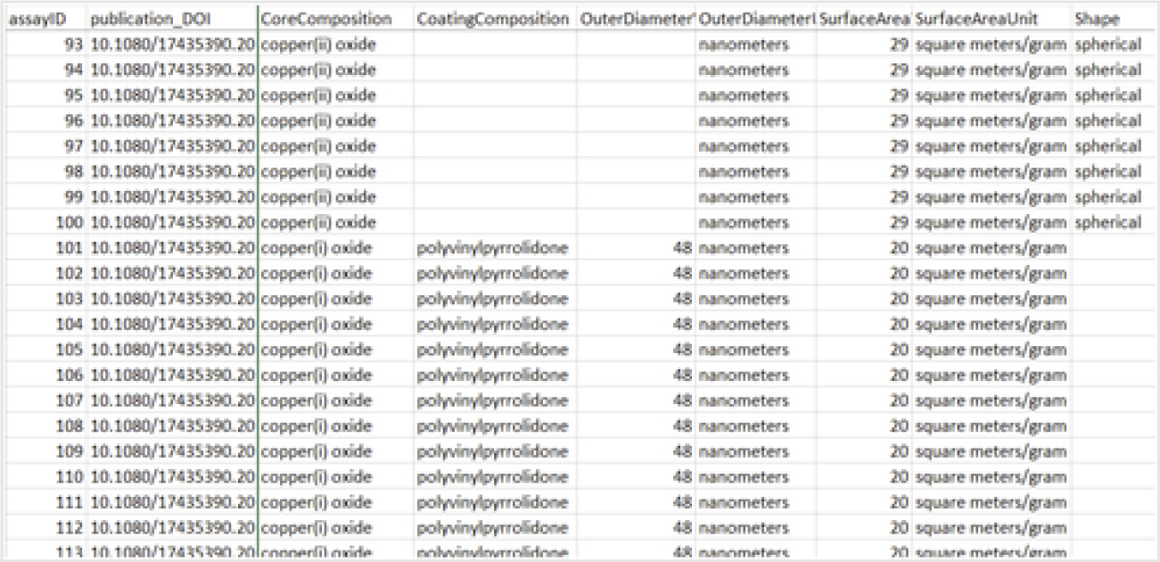
NKB in spreadsheet format: data in NKB can be read, pre-processed, and analysed in a spreadsheet format.

Pre-processing data from NKB

Often there are many records in a relational database table that may be associated with the same assay sample. For example, a particular nanomaterial investigation may have several records from Table 3. Additives in the medium of an in vitro assay. To contain all the additive information in a single row, all the fields of each additive record are concatenated together in mySQL and put into the CSV file as a single column entry with the different field values divided by colons (“:”). Once in Python, the CSV file is read into pandas dataframe using the pandas.read_csv()²⁴ function. Using pandas dataframe, these concatenated entries with colons are deconcatenated and expanded into appropriate newly created columns of the dataframe. In this way, all the concatenated entries from the multiple records of the parameters, additives, contaminants, and results tables are deconcatenated and expanded into the correct columns of the refined spreadsheet.

Table 3.

Additive table data fields: additives to a medium were recorded in the additive table. Entries in this table were comprised of the DOI and MediumID of the medium in question, the name of the substance being added, the amount being added, and the units. A medium could have any number of additives, including zero

Additive table	Description
AdditiveID	Unique (within publication) numerical identifier to link an additive to entries in other tables
Additive	Name of additive
Concentration	Concentration of additive
Units	Units of additive
medium_MediumID	Reference to medium ID of the medium this additive was added to
medium_publication_DOI	Reference to DOI of medium’s source publication

In coordination with the published conventions of the eNanoMapper^19,20 ontologies, NKB was designed to accept, maintain, and use terminology consistent with expanded nanomaterial ontologies developed by nanoinformatics groups including the EU NanoSafety Cluster and the Center for the Environmental Implications of Nanotechnology (CEINT). One of these ontologies allow values to be entered along with their associated units of measure. Both values and their associated units of measure are retained in two separate columns of the NKB. Before QSAR analysis can be done, any entries in the same column that have different units in different rows must be converted, so that all entries in the same column have the same unit (e.g., values with μm unit are converted to values with nm unit). This same process must be performed for all columns that have different units in different rows. All unit conversions needed were written into the pre-processing software to ensure this.

A column that contains categorical data can greatly enhance QSAR analysis. For example, NKB contains the assay results of exposure to ENMs of different core compositions (CoreComposition). The OneHotEncoder (https://scikit-learn.org/stable/modules/generated/sklearn.preprocessing.OneHotEncoder.html) is a binary encoder routine in sklearn that creates a new column for each type of core composition found. Each sample/row that has a core composition of a certain type has a 1.0 in that column and a 0.0 in the others. After this, the original categorical column is no longer needed and can be deleted.

This binary encoder works well for categorical columns that have relatively few types. When a categorical column has many types, this process creates too many new columns and sklearn’s LabelEncoder is used instead. This converts a categorical column of many types into a column of many integers in a simple one-to-one fashion.

All the pre-processing steps examined so far share the common problem of containing many empty and blank fields. An important final step of pre-processing is to approximate these values wherever possible using imputation. However, different empty or blank fields are handled differently. For example, the sizes of nanomaterial clusters investigated are given by the related OuterDiameterValue, OuterDiameterLow, and OuterDiameterHigh columns. Entries in these columns that are missing or blank are approximated by values in these related columns that are available. For example, if OuterDiameterValue is blank, it is approximated as an average between the values in the OuterDiameterLow and OuterDiameterHigh columns. A missing or blank entry in a “Temperature” column is entered as a room temperature of 25 °C.

When chemical contaminants are found in the ENMs studied in NKB, a column is created for each contaminant found with a row value that represent the concentration of that contaminant. Row values that are not in the mixture are replaced with concentrations of 0.0. This same process can be carried out for studies contained in NKB that have additives found in the medium of the assays conducted.

At some point in the pre-processing of rows and columns, it is helpful to remove rows that are not used building a particular QSAR analysis model. For example, the assays conducted by ORD scientists and curated into NKB may measure completely different effects from exposure to nanomaterials. Only the rows that measure the same effects can be used to build and test models to predict that effect. Any row in the spreadsheet data that does not contain this measured effect is not used and is deleted. Similarly, when all the values in a column are the same, the column does not contribute to building the model, and it is deleted.

As shown above, pre-processing of the data mined from NKB can be a very long and difficult task. However, anytime sample rows are saved by imputing values rather than throwing them away because of unknown values, the relationships between the independent and dependent values are improved. This process greatly assists the scientist datamining NKB, and it significantly improves the data available for QSAR analysis.

QSAR analysis

Dependent and independent variables

By processing the informatics data contained in databases, regression analysis algorithms can be used to build and test models that determine relationships between independent variables and their predicted dependent targets. Exactly how successful models are at making such predictions is frequently measured by the coefficient of determination²⁵ which is a function of the difference between the predicted and observed values of a targeted dependent variable as shown in eqn (1).

The targeted variable in this paper is the viability of cell cultures after being exposed in vitro to different forms and concentrations of ENMs for different periods of time and under different laboratory conditions. However, the results of many more USEPA/ORD peer-reviewed studies^9–14 of types in vitro, in vivo, life cycle and more have been curated into NKB for future examinations.

The core compositions of ENMs investigated for this QSAR analysis are cerium oxide(IV), copper(I) oxide, copper(II) oxide, silver, titanium dioxide, zinc oxide, and negative controls where no ENM is present. The in vitro assays curated into NKB are human cell types ARPE-19, E6–1, HEPG2 and SMI-100, and rat cell type IEC-6.

There are a total of 60 independent variables that are available for examination. For example, the coating compositions of ENMs investigated are aluminium hydroxide, citrate, polyvinylpyrrolidone, and no coating. Independent variables are included for analysis such as the duration of exposure to the ENMs in hours, the outer diameter size of the ENMs in nanometers, the concentration of the ENMs given in micrograms/milliliter, the surface area given in square meters/gram, a surface area charge of type zeta potential given in millivolts, and more. The values of these independent variables are taken from samples within NKB to build models. Likewise, they may be set and varied by researchers to test and investigate consequences in the dependent targets.

The forest of decision trees

The QSAR analysis tool implemented is the RandomForestRegressor routine taken from sklearn. This routine builds a model from a forest of decision trees grown from training samples with a default size of 100 trees. The model then makes predictions by taking the average of the predictions made by every tree in the forest. This prediction not only has an average, but it has an uncertainty associated with that prediction as well.

Each tree in the random forest is started and grown from a bootstrapped selection of 80% of the training samples. At each branch of a tree, a feature is chosen that divides the selected set of samples up to reduce the uncertainty of the target values the most. This branching continues all over the tree until each branch has less than four samples (min_samples_split=4). Then branching stops and only leaves remain, where each leaf contains every training sample that followed the same branches down the decision tree to the same endpoint.

The target value of any new sample may then be predicted by proceeding down the branches in each tree based upon the values of the new sample’s features. This journey continues down the branches until the leaf is reached. The target value can then be given by taking the average of the target value over all the training samples that end at the same leaf. As mentioned before, a similar prediction process can be done by each tree in the forest independently. This gives a predicted value average over all trees in the forest, along with an associated uncertainty of the prediction.

The cross-validation process

A common process for testing the accuracy of QSAR models is to cross-validate the methods used to build the models. This was done using a k-fold method where the samples used to train and test models are randomly split up into $k$ groups or folds. For $i=1,k$ steps, the ith fold of samples is used for testing, and the other $k-1$ folds of the samples are used for training. A metric used to represent the accuracy of a model fit is the quantity $R^2$, which is known as the coefficient of determination²⁵ and is represented by eqn (1).

$$R^2=1-\frac{{\mathrm{S}\mathrm{S}}_{\text{res}}}{{\mathrm{S}\mathrm{S}}_{\text{tot}}}$$ 1

where ${\mathrm{S}\mathrm{S}}_{\text{res}}$ is the residual sum of squares given by:

$${\mathrm{S}\mathrm{S}}_{\mathrm{r}\mathrm{e}\mathrm{s}}=\sum _{i=1}^n{\left(y_i-f_i\right)}^2=\sum _{i=1}^n{\mathrm{e}}_i^2$$

and ${\mathrm{S}\mathrm{S}}_{\text{tot}}$ is the total sum of squares given by:

$${\mathrm{S}\mathrm{S}}_{\text{tot}}=\sum _{i=1}^n{\left(y_i-\bar{y}\right)}^2$$

Here, $\left\{y_1,y_2,\dots ,y_n\right\}$ are the observed values, $\left\{f_1,f_2,\dots ,f_n\right\}$ are the predicted values, and $\bar{y}$ is the average observed̄ value. In the best case ${\mathrm{S}\mathrm{S}}_{\mathrm{r}\mathrm{e}\mathrm{s}}=0$, so that $R^2=1$.

Cross-validating the process of building a random forest of decision trees to predict the viability of cells expose to different types of ENMs under various laboratory conditions proved to be interesting. The $R^2$ value for the training set used to build the random forest of decision trees is usually closer to 1 and represent how much over-fitting has occurred during the model building. The $R^2$ value for the test set better represent the accuracy of the model for all new predictions. A 5-fold splitting of all the samples achieved an average of $R^2=0.87\pm 0.01$ on the training sets and an average of $R^2=0.67\pm 0.06$ on the test sets.

A final test

All the samples were randomly split 20% into a test set and the remaining 80% into a training set. The test set was retained so that predictions for it could be repeated and compared in future studies. The model, a forest of 100 decision trees, created by the training set predicted the viabilities of the training set with a coefficient of determination accuracy of R² = 0.88. A high value is not uncommon when predicting the target values of samples used to build a model. The same model predicted the test set viabilities with an accuracy of $R^2=0.68$.

The Jaqpot cloud platform

While building, training, and testing models can be carried out by researchers using tools specific to their studies, it is also necessary to make similar tools available to other modelers to verify findings and to follow-up with additional discoveries. An efficient way to share models that have been developed by researchers is by accessing the Jaqpot cloud platform (https://app.jaqpot.org/)²² developed by the National Technical University of Athens (NTUA), Greece. The important Jaqpot tutorials (https://zenodo.org/record/4671074/preview/JPQ5_UI_TUTORIAL_NTUA_ModelUse_08042021.pdf)²⁶ to assist opening and using this site are available for reading or downloading.

One of the main purposes of this platform is to share nanoinformatics models to predict nanoEHS effects. NanoEHS researchers may deploy models and databases constructed by others on this platform to make QSAR predictions about ENMs. Likewise, nanoinformatics QSAR researchers can create and upload their own models and databases using this platform to share their nanoEHS data with others.

The first step for gaining access to the Jaqpot cloud platform is to acquire a login name and password. Fig. 3 presents the Jaqpot landing page, accessed using a Chrome browser. Login names and password may be assigned to institutes such as the US EPA to use collectively, or to individual users. Once a login name and password have been secured, the Jaqpot cloud platform can be accessed over the internet.

Fig. 3.

Jaqpot cloud platform: Jaqpot login website https://app.jaqpot.org/. ²²

Once an individual has logged into this Jaqpot cloud platform, they will immediately be taken to Home directory with a Quick view of private models that have been saved for additional modeling as shown in Fig. 4. The models listed can be selected to view by clicking on the “eye” that appears when the cursor floats over the model listed. Or the model can be deleted when clicking on the “trash can”.

Fig. 4.

Jaqpot home site, quick view: Home page showing private models available for a quick view.

Additional models that are shared by other researchers may be accessed by clicking on the “Models Shared/Private” button listed in the left column and choosing “Shared” from the drop-down menu that appears when selecting the right-most arrow in the script at the top of the screen as shown in Fig. 5.

Fig. 5.

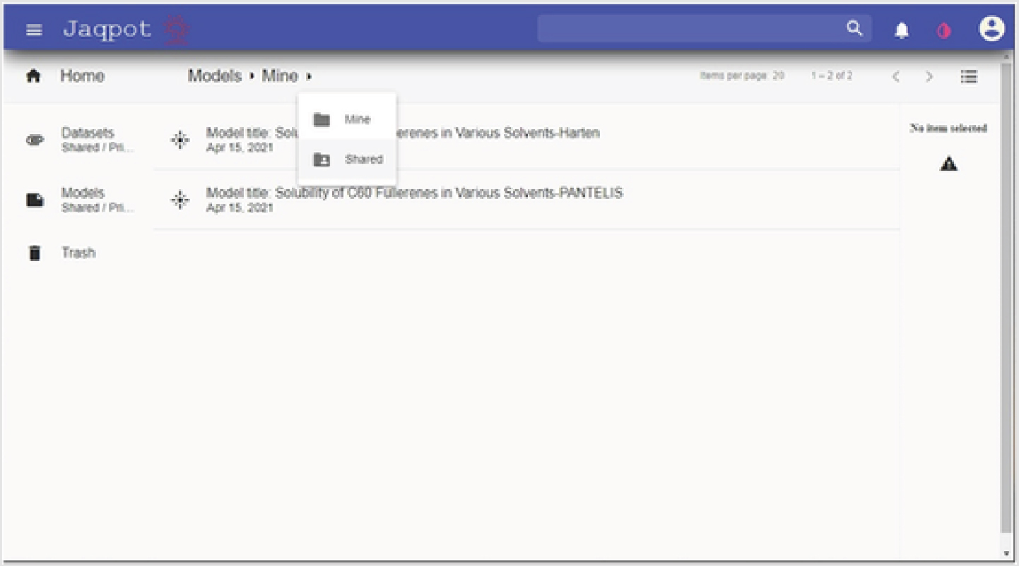
Jaqpot home site, shared models: home page showing how to access shared models.

One of the choices of shared models are those shared “With EPA”. The shared models listed in Fig. 6, and more are a result of a collaboration between US EPA and NTUA. Most of these QSAR models were generated by NTUA using the US EPA database NKB. However, many datamining and pre-processing steps were necessary to refine NKB data for QSAR analysis. A model near the bottom of Fig. 6 is highlighted with the abbreviated title “EPA model for nanomaterial viability prediction”. The pre-processing and QSAR predictions performed by the viability model are discussed extensively in this article. It may be used to predict the in vitro viability of the five different cell types mentioned separately after being exposed to certain kinds of ENMs.

Fig. 6.

Models shared with EPA: list of shared models with EPA model for nanomaterial impacts on cell viability prediction highlighted.

By clicking on the “eye” icon of the selected model, the user is taken to another screen where information about this model is shown. This new screen is an overview of the viability model. As shown in Fig. 7, various points of information about the model are displayed such as: 1) how many features are required as input for this model; 2) how many observations were used in the training sample; 3) the developer of the model; 4) the name of the database where the samples originated; and 5) a general synopsis of the model’s prediction. By using the scroll bar on the right side of the screen, much more information about the viability model can be seen.

Fig. 7.

Overview of the EPA model for viability prediction: complete information, metrics, and values of the viability prediction model are displayed online.

At the top of the screen in Fig. 7, there is a command bar that allows access to different functions associated with the viability model. The command bar is currently showing the Overview function. Clicking on other items in the command bar allows access to other functions. For example, clicking on the “Features” function takes the user to the Features screen as shown in Fig. 8.

Fig. 8.

Features of the EPA model for viability prediction: the dependent or predicted variable and the independent variables of the model are listed. The term “ missing” appears in the names of some of the independent features as a result of using the routine OneHotEncoder (https://scikit-learn.org/stable/modules/generated/sklearn.preprocessing.OneHotEncoder.html) on possible entries of categorical data.

This is a listing of the dependent feature to be predicted which in this case is the viability_result_value. This is also a listing of the independent variables used in the model to make the model prediction. As before, by using the scroll bar on the right side of the screen, more independent variables of the viability model can be viewed.

The next function of interest in the command bar is the “Predict/Validate” function. Selecting this feature brings up a screen as shown in Fig. 9. This screen allows predicting or validating the viability of a cell type when exposed to a certain nanomaterial under specific in vitro conditions. It allows a prediction to be made by choosing the method “Predict” and filling in values for the independent variables. After all values are filled in, a start button appears. Clicking on this button starts the process and shows different steps of calculation that are listed as tasks begin. Once all tasks have completed successfully, a double checkmark icon appears. The predicted viability of a cell type exposed to the ENM of interest appears after choosing this checkmark.

Fig. 9.

Predict viability of nanomaterials: input the values of independent variables to calculate the viability of nanomaterials.

An alternate and easier way to make many predictions at the same time is to download a CSV file with headers for each column to show the same independent variable entries that are needed for predictions. By selecting the down arrow shown in Fig. 9, a window appears prompting for a filename and a directory where to place this prediction template CSV file. An example of a downloaded prediction template file with filled in values is given in Fig. 10. This is an attempt at using the EPA model for ENM viability prediction to predict how in vitro cell viability changes with different particle concentrations of a specific type of ENM.

Fig. 10.

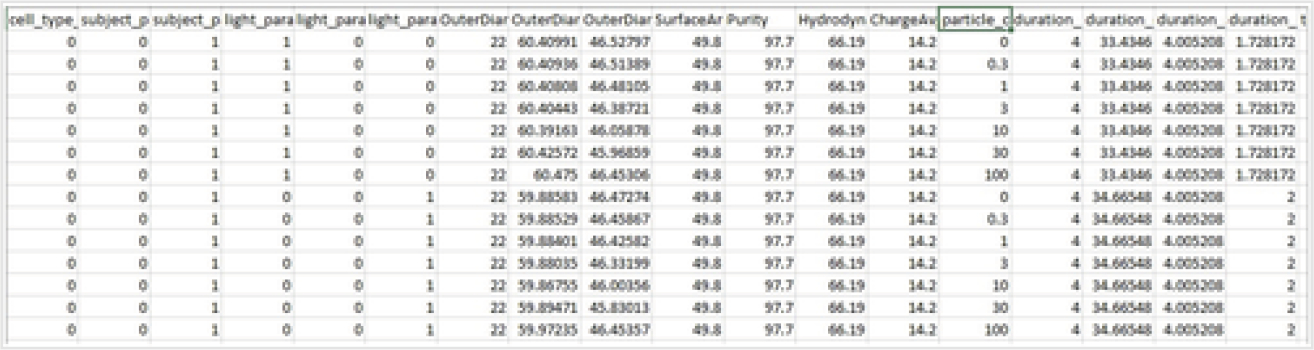
Uploading entries for multiple predictions: many nanomaterial viability predictions may be calculated at the same time by downloading the CSV prediction template, entering values, uploading the entries, and selecting predict.

After such a CSV file is generated, it can be uploaded to Jaqpot’s prediction/validation page by selecting the up arrow shown in Fig. 9. A file with the entries for ARPE-19 cell cultures exposed to various particle concentrations of ENM titanium dioxide under different lighting conditions is in the EDG²³ with the filename TitaniumDioxide_ARPE_19.csv. The new dataset will appear on the screen when it is finished uploading with a button to start the procedure of calculating the viability predictions. As described before, each step of the tasks involved with the QSAR predictions will be listed during calculations. Upon successful completion, a double checkmark will appear to view viability predictions, and to download all values including the predicted values to a local file. If the download is accepted, the user will have a local CSV file like the one uploaded but with an additional column with the header “viability_result_value” where the dependent predicted values are placed based with the values of all the independent variables in the same row.

Validation of predicted values can also be performed by choosing the method “Validate” instead of “Predict” in the upper part of the screen shown in Fig. 9. The same upload and download processes can be chosen to move CSV data files from local input resources to remote model calculation resources. However, once the “Regression Validation method” and the “Start Procedure” buttons have been chosen and calculations have completed, a more formal Validation report can be viewed through the browser showing not only R² and StdError values but also graphs displaying a QQ quantile plot and a real vs. predicted values plot with an identity line and 95% confidence level lines. This last plot is shown in Fig. 11. More detailed descriptions of the Jaqpot prediction and validation processes can be found in the tutorial “Jaqpot 5: how to access and use an existing predictive model”.²⁶

Fig. 11.

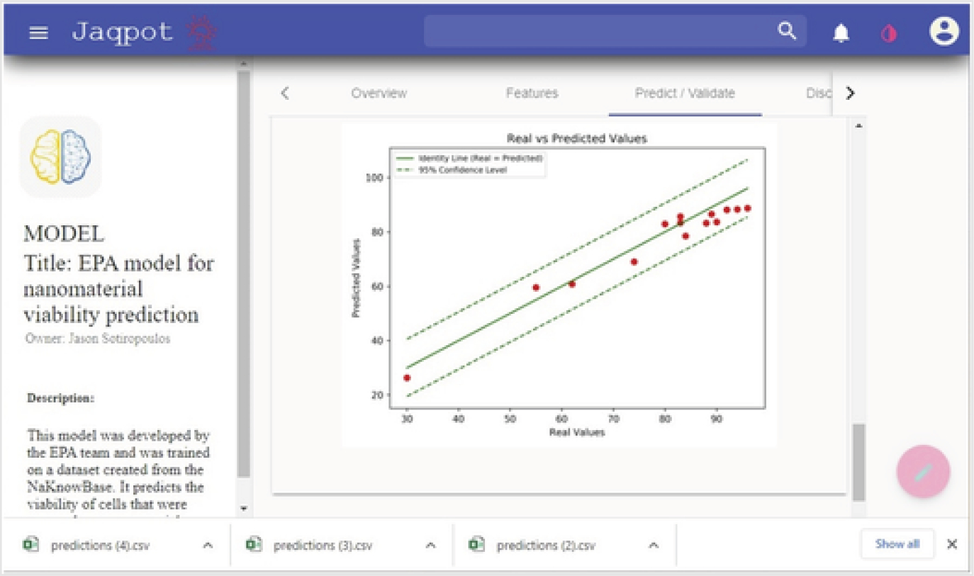
Validation of EPA model report: validation of models may be selected resulting in a report containing measures of accuracy and real vs. predicted plots.

The last section of this article shows how to predict and validate using local resources for both data input and saving results as shown in Fig. 10, and using remote resources for calculations and modeling as shown by the screenshots displayed in Fig. 3–9 and 11. However, there are many other operations that can be performed on the Jaqpot website (https://app.jaqpot.org/)²² that have not been reviewed. Uploading models and databases developed by researchers to share with others is also a practical capability of this platform. This capacity will become a subject of future investigations.

Summary

Because of the ENM wastes released during manufacturing and using ENMs, it is important to find ways to safely protect human health and the environment. Experimentalists lead this effort by conducting assays that explore the consequences of exposure to ENMs under specific conditions and publish their results. Such publications require extensive details about the ENM, laboratory conditions, and experimental effects that can be used and confirmed by others.

Publications by ORD nanomaterial researchers investigating the fate and effects of ENMs across their life cycle have been reviewed and curated to build the EPA database, NaKnowBase (NKB). Extensive efforts have been coordinated to datamine NKB and refine the data taken to support QSAR predictions of these harmful side effects for similar nanomaterials. In particular, the EPA model nanoQSAR predicts impacts to in vitro cell viability following exposure to certain nanomaterials.

A web-based method to confirm predictions of the in vitro viability of different cell types after exposure to ENMs is presented here implementing the Jaqpot cloud platform created and supported by NTUA, Greece. The EPA nanoQSAR predictor as well as many other QSAR predictors developed by NTUA that use NKB have been made possible by an international NanoCommons collaboration between the USEPA and NTUA.

Methods used to mine and refine the data within NKB to predict the harmful side effect of nanomaterials have been discussed in this article. These methods can be used by computational environmental scientists everywhere with access to NKB to investigate other harmful side effects created in the life cycle of nanomaterials.

Table 4.

Contam table data fields: the contaminants table, “contain”, served as an addendum to the material table. The primary key was comprised of the publication DOI and MaterialID of the contaminated material. The field contaminant listed the name of the contaminating substance. ContamAmount, ContamUnit, and ContamMethod held the information on the scale of the contaminant and the way the contamination was measured. This allowed for a material to have any number of contaminants, each detailed in its own row

Contam (contaminants) table	Description
ContamID	Unique identifier for the contaminant data point
material_MaterialID	Reference to material ID of the material in which this contaminant was found
material_publication_DOI	Reference to DOI of source publication
Contaminant	Chemical identity of the contaminant
ContamAmount	Measured numerical amount of the contaminant
ContamUnit	Units of measurement of contaminant (e.g., %, units of mass per volume)
ContamMethod	Analytical method to identify and measure the contaminant (e.g., ICP-MS, etc.)

Environmental significance.

Progress in the area of computational toxicology has been hampered by poorly structured and fragmented data. Additionally, the study of nanomaterials has been challenged by nomenclature inconsistencies. The EPA NaKnowBase was developed to better characterize nanomaterials of environmental and human health concern. In this manuscript, Harten et al., present the EPA nanoQSAR tool, and implement the tool in QSAR modeling and analysis of the NaKnowBase data. In conjunction international colleagues at the National Technical University of Athens, Harten et al. use nano-QSAR outputs to estimate in vitro cell viability following nanomaterial exposure, further underlining the utility and importance of this contribution. These collaborative efforts contribute to the improved FAIR data standards for nanomaterials data through data accessibility, interoperability and re-use.

References

- 1.Kilby JS, Invention of the integrated circuit, IEEE Trans. Electron Devices, 1976, 23, 7, 648–654, DOI: 10.1109/T-ED.1976.18467. [DOI] [Google Scholar]
- 2.Iijima S, Helical microtubules of graphitic carbon, Nature, 1991, 354, 56–58, DOI: 10.1038/354056a0. [DOI] [Google Scholar]
- 3.Oberlin A, Endo M and Koyama T, Filamentous growth of carbon through benzene decomposition, J. Cryst. Growth, 1976, 32, 3, 335–349, DOI: 10.1016/0022-0248(76)90115-9. [DOI] [Google Scholar]
- 4.Sreenivasan M, Cytology of a Spontaneous TriploidCoffea CanephoraPierre ex Froehner, Caryologia, 1981, 34, 3, 345–349, DOI: 10.1080/00087114.1981.10796901. [DOI] [Google Scholar]
- 5.Cao Y, Fatemi V and Fang S, et al. , Unconventional superconductivity in magic-angle graphene superlattices, Nature, 2018, 556, 43–50, DOI: 10.1038/nature26160. [DOI] [PubMed] [Google Scholar]
- 6.Haase A and Klaessig F, EU US Roadmap Nanoinformatics 2030, 2018, https://zenodo.org/record/1486012#.Xp9cm8hKg2w
- 7.National Science and Technology Council, Commitee on Technology and Subcommittee on Nanoscale Science, Engineering, and Technology, National Nanotechnology Initiative Environmental Health, and Safety Research Strategy, 2011, https://www.nano.gov/sites/default/files/pub_resource/nni_2011_ehs_research_strategy.pdf.
- 8.Afantitis A, et al. , NanoSolveIT Project: Driving nanoinformatis research to develop innovative and integrated tool for in silico nanosafety assessment, Comput. Struct. Biotechnol. J, 2020, 18, 583–602, DOI: 10.1016/j.csbj.2020.02.023. [DOI] [PMC free article] [PubMed] [Google Scholar]
- 9.Thai SF, Jones CP and Nelson GB, et al. , Differential Effects of Nano TiO2 and CeO2 on Normal Human Lung Epithelial Cells In Vitro, J. Nanosci. Nanotechnol, 2019, 19, 11, 6907–6923, DOI: 10.1166/jnn.2019.16737. [DOI] [PMC free article] [PubMed] [Google Scholar]
- 10.Al-Abed SR, Virkutyte J and Ortenzio JNR, et al. , Environmental aging alters Al(OH)3 coating of TiO2 nanoparticles enhancing their photocatalytic and phototoxic activities, Environ. Sci.: Nano, 2016, 3, 593, DOI: 10.1039/c5en00250h. [DOI] [Google Scholar]
- 11.Prasad RY, McGee JK and Killius MG, et al. , Investigating oxidative stress and inflammatory responses elicited by silver nanoparticles using high-throughput reporter genes in HepG2 cells: Effect of size, surface coating, and intracellular uptake, Toxicol. In Vitro, 2013, 27, 6, 2013–2021, DOI: 10.1016/j.tiv.2013.07.005. [DOI] [PubMed] [Google Scholar]
- 12.Ivask A, Scheckel KG and Kapruwan P, et al. , Complete transformation of ZnO and CuO nanoparticles in culture medium and lymphocyte cells during toxicity testing, Nanotoxicology, 2017, 11, 2, 150–156, DOI: 10.1080/17435390.2017.1282049. [DOI] [PMC free article] [PubMed] [Google Scholar]
- 13.Henson TE, Navratilova J, Tennant AH, Bradham KD, Rogers KR and Hughes MF, In vitro intestinal toxicity of copper oxide nanoparticles in rat and human cell models, Nanotoxicology, 2019, 13, 6, 795–811, DOI: 10.1080/17435390.2019.1578428. [DOI] [PMC free article] [PubMed] [Google Scholar]
- 14.Sanders K, Degn LL and Mundy WR, et al. , In Vitro Phototoxicity and Hazard Identification of Nano-scale Titanium Dioxide, Toxicol. Appl. Pharmacol, 2012, 258, 2, 226–236, DOI: 10.1016/j.taap.2011.10.023. [DOI] [PubMed] [Google Scholar]
- 15.Boyes WK, et al. , A comprehensive framework for evaluating the environmental health and safety implications of engineered nanomaterials, Crit. Rev. Toxicol, 2017, 47, 767–810, DOI: 10.1080/10408444.2017.1328400. [DOI] [PubMed] [Google Scholar]
- 16.Boyes WK, Beach B, Chan G, Thornton BLM, Harten P and Mortensen HM, An EPA database on the effects of engineered nanomaterials-NaKnowBase, Sci. Data, 2022, 9, 1, 12, DOI: 10.1038/s41597-021-01098-0. [DOI] [PMC free article] [PubMed] [Google Scholar]
- 17.Bayer M, SQLAlchemy, The Architecture of Open Source Applications Volume II: Structure, Scale, and a Few More Fearless Hacks, ed. Brown A and Wilson G, 2012, https://aosabook.org/en/v2/sqlalchemy.html [Google Scholar]
- 18.Pedregosa[Instruction: F. Pedregosa], et al. , Scikit-learn: Machine Learning in Python, J. Mach. Learn. Res., 2011, 12, 2825–2830, https://jmlr.csail.mit.edu/papers/v12/pedregosa11a.html [Google Scholar]
- 19.Jeliazkova N, et al. , The eNanoMapper database for nanomaterial safety information, Beilstein J. Nanotechnol, 2015, 6, 1609–1634, DOI: 10.3762/bjnano.6.165. [DOI] [PMC free article] [PubMed] [Google Scholar]
- 20.Hastings J, et al. , eNanoMapper: harnessing ontologies to enable data integration for nanomaterial risk assessment, J. Biomed. Semant, 2015, 3, 6–10, DOI: 10.1186/s13326-015-0005-5. [DOI] [PMC free article] [PubMed] [Google Scholar]
- 21.EPA GitHub Repository, nanoQSAR, Retrieved: April 06, 2023 from https://www.github.com/usepa/nanoQSAR
- 22.Sarimveis H, et al. , The Jaqpot Cloud Platform, Developed by the Unit of Process Control and Informatics at the National Technical University of Athens, Greece, 2022, https://app.jaqpot.org/
- 23.Harten P, et al. , EPA’s Environmental Dataset Gateway for nanoQSAR, U.S. EPA Office of Research and Development (ORD), 2023, Clowder Link https://clowder.edap-cluster.com/datasets/61147fefe4b0856fdc65639b#folderId=648b4582e4b08a6b394ef1fd&page=0 [Google Scholar]
- 24.Reback J, et al. , pandas-dev/pandas: Pandas 1.4.2, 2022, 10.5281/ZENODO.6408044, https://pandas.pydata.org/docs/reference/api/pandas.read_csv.html [DOI]
- 25.Coefficient of determination, Wikipedia, 2023, https://en.wikipedia.org/wiki/Coefficient_of_determination
- 26.Sarimveis H, et al. , PQ5_UI_TUTORIAL_NTUA_ModelUse, 2021, https://zenodo.org/record/4671074/preview/JPQ5_UI_TUTORIAL_NTUA_ModelUse_08042021.pdf